| Issue |
A&A
Volume 707, March 2026
|
|
|---|---|---|
| Article Number | A63 | |
| Number of page(s) | 7 | |
| Section | Cosmology (including clusters of galaxies) | |
| DOI | https://doi.org/10.1051/0004-6361/202557012 | |
| Published online | 26 February 2026 | |
More power on large scales
1
Swinburne University PO Box 218 Hawthorn 3121, Australia
2
ARC Centre of Excellence for Dark Matter Particle Physics Victoria 3010, Australia
★ Corresponding author: This email address is being protected from spambots. You need JavaScript enabled to view it.
Received:
28
August
2025
Accepted:
11
January
2026
Abstract
The high value of the cosmic microwave dipole may be telling us that dark matter is macroscopic rather than a fundamental particle. The possible presence of a significant dark matter component in the form of primordial black holes (PBHs) suggests that simulation of dark halo formation should be commenced well before redshift z = 100. Unlike standard cold dark matter candidates, which are initially relativistic or possess thermal velocities, PBHs behave as dense non-relativistic matter from their inception in the radiation-dominated era. This allows them to seed gravitational potential wells and begin clustering much earlier, which significantly alters the initial power spectrum on small scales. We find that when we start N-body simulations at redshifts even before matter-radiation equality (z ∼ 3400), the galaxy bulk flow velocities are systematically higher than those predicted by standard ΛCDM models. The early high-mass concentrations established by PBHs lead to a more rapid and efficient gravitational acceleration of the surrounding baryonic and dark matter and generate higher peculiar velocities that remain coherent over scales of hundreds of megaparsec. Furthermore, a sub-population of PBHs in the 10−20 to 10−17 M⊙ mass range would lose a non-negligible fraction of their mass via Hawking radiation over cosmological timescales. This evaporation process converts matter into radiation, so that a time-varying matter density parameter, Ωm′, is introduced that behaves like a boosted radiation term, in the Friedmann equation. This dynamic term, which is most active between recombination and the late Universe, acts to reduce the Hubble tension. A higher effective Ωr in the early Universe (pre-evaporation) reduces the sound horizon at the epoch of recombination. This smaller standard ruler as imprinted on the cosmic microwave background (CMB) would result in a higher value of the Hubble constant (H0) inferred from the CMB at the 1% level, which brings it into slightly closer agreement with local late-time measurements. PBH mass loss also affects fits to the equation of state parameter w at low redshift. The naive N-body modelling presented here suggests that an investigation with tried and tested cosmology codes should be carried out by introducing mass-losing PBHs and starting the evolution as early as practicable.
Key words: cosmological parameters / large-scale structure of Universe
© The Authors 2026
 Open Access article, published by EDP Sciences, under the terms of the Creative Commons Attribution License (https://creativecommons.org/licenses/by/4.0), which permits unrestricted use, distribution, and reproduction in any medium, provided the original work is properly cited.
This article is published in open access under the Subscribe to Open model. This email address is being protected from spambots. You need JavaScript enabled to view it. to support open access publication.
1. Introduction
Ever since peculiar velocities have been measured for galaxies, it has been noted that standard cosmological models lack sufficient power on large scales (Aaronson & Olszewski 1988; Dekel 1993; Lauer & Postman 1994; Tully 1989; Hudson et al. 2004; Watkins et al. 2023; Whitford et al. 2023; Böhringer et al. 2025; Secrest 2025; Watkins & Feldman 2025). Bouillot et al. (2014) reported that the large bulk flow is due to an asymmetric distribution of matter, a rare event that would occur in the ΛCDM cosmology 1.4% of the time. Although the research is almost unanimous1 on this issue, cosmological models that satisfy the constraint have not, with the possible exceptions of neutrinos and modified gravity2, been forthcoming. Tsagas et al. (2025) provided the most recent review. Even though the statistics will soon be overwhelming due to the WALLABY survey (Widefield ASKAP L-band Legacy All-sky Blind surveY, Colless 2024), the DESI (Dark Energy Survey Instrument) DESI Collaboration (2025), and 4HS (4MOST Hemisphere Survey, Taylor 2023), there remain issues, such as the Malmquist bias, that can afflict the data.
I offer a toy model that does develop higher velocities by employing mass-losing dark matter and an early phase of high density (Section 2). If the dark matter (DM) particle were in fact unstable, the decay products might be observed as an excess in the cosmic-ray fluxes of antimatter particles, γ-rays, or neutrinos over the expected backgrounds. Many experiments have provided data of exquisite quality on the cosmic antimatter, γ-ray, and neutrino fluxes, which allow us to set independent limits on the DM decay width into a given final state. When we focus on DM particles with masses in the GeV–TeV range, the σv cross sections of masses, m, from 10−2 to 107 GeV are lower than 10−22 cm3 s−1 (Pérez de los Heros 2020). With v2 = 2 kT/m the decay rate, n σv for keV intergalactic medium temperatures and densities is lower than 10−25 s−1, and for interstellar medium meV temperatures and GeV/cm3 densities, it is lower than a hundredth of this. DM particles in this range would therefore be stable at cosmic densities for a Hubble time. The DM decay beyond the standard model is still open to investigation, however (e.g. Poulin et al. 2017).
Primordial black holes (PBHs), on the other hand, also decay into high-energy photons and PeV to meV particles, depending on their mass, but experimental constraints have left open significant windows, notably between 10−16 and 10−8 M⊙. PBHs with m < 10−19 M⊙ evaporate within a Hubble time (Mosbech & Picker 2022; Mould 2025). In Section 3 we normalise the toy model to observations. The simulated bulk flows are discussed in Section 4. Inman & Ali-Haïmoud (2019) have also explored early structure formation by PBH.
2. A toy model
The best-motivated candidates for mass-losing DM are PBHs in the mass range of 10−20–10−17 M⊙, which would be losing mass via Hawking radiation on cosmological timescales (Figs. 1 and 2). The first of the transitions (dotted lines in Figure 1) is discussed as a possible PBH trigger by Alonso-Monsalve & Kaiser (2023). As the Universe cools, the lowest-mass PBHs take a right angle turn to high temperatures, rapidly becoming Planck mass relics. Higher masses than those in Figure 1 are shown by Mould (2025).
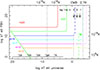 |
Fig. 1. Temperature evolution of low-mass PBHs vs. cosmic temperature. In the radiation-dominated era, PBHs of mass 10−23 M⊙ (denoted m23) and higher, if they form, do so on the green diagonal line and evolve with little mass loss until Ṁ is of the same order as M, at which point they rapidly heat and evaporate. Kelvin units are used at the top and right borders. PBHs change their evolutionary rate as T ∼ M−1, from radiation (solid line), to matter (dashed line), to dark-energy dominated (dotted line). The t8 line marks the start of galaxy formation. The three dotted vertical lines are from left to right the QCD transition at 220 MeV, the surface of last scattering of the CMB, and the temperature today, 2.7 K. |
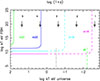 |
Fig. 2. Enlargement of Fig. 1 for z < 105. Redshift log(1+z) is denoted by the numbers towards the top. The CMB is shown by the vertical dotted line, and 108 years is shown by the vertical dashed green line. |
A number of 256 000 particle n-body runs were made, whose details are listed in Table 1 and whose final velocity distribution functions are given in the appendix. These are DM-only simulations. The run numbers are an internal reference code. The numerical resolution is a minimum particle distance of 10−20. The PBHs expand with the Hubble flow. Black hole mergers were not treated, as they only become significant at supersolar PBH masses, where the geometrical cross sections exceed 1 cm2. The initial conditions were a uniform random distribution of particles at rest in a sphere with a nucleus of mass m, the largest in the distribution. The simulations were scale free in radius, mass, and velocity. The IMF was a top hat in log m, with the lowest and highest mass shown as m1 and m2. Mould & Hurley (2025) have shown that the IMF in the case of supermassive black holes yields the observed QSO luminosity function. The baryons were not considered in these calculations3.
N-body simulations.
The toy model was implemented within a scale-free framework, which means that absolute masses, distances, and velocities were unspecified, but their ratios and the statistical properties of the density field are meaningful and can be scaled to any epoch in which matter dominates. To quantify the resulting velocity field, we calculated the bulk flow from the particle velocity array. The median velocity was adopted as the primary statistic rather than the mean or rms because it is more robust against spurious high-velocity outliers generated by close two-body encounters, an unphysical artefact of N-body simulations at scales below the gravitational softening length.
Mass loss was implemented in the toy model via two distinct prescriptions: (1) by dynamically reducing all particle masses according to the PBH evaporation rate (Ṁ ∝ M−2), as formulated in Mosbech & Picker (2022), and (2) by a more phenomenological approach in which instead of tracking individual particle masses, we stochastically removed a fixed percentage of particles from the phase-space arrays at each timestep. For simplicity, a spatially flat geometry (Ωk = 0) was assumed at all times, and simulations ceased at a redshift of at z ≈ 1, the approximate epoch at which dark energy begins to significantly affect the cosmic expansion rate and tends to suppress the self-similar growth of structure.
The final large-scale structure is illustrated in Fig. 3. Even though these simulations have fewer particles by some orders of magnitude, the familiar cosmic web can be traced together with mass concentrations. The limitations of the toy model are that there are no baryons, and therefore, the stronger mass concentrations produced by baryonic collapse and cooling is not seen. The velocity distribution of particles in runs 104–107 is shown in the appendix. The velocity dispersions are spatially uniform except in the outer parts of the simulations, where particles that have had strong interactions are escaping. These number under 1000 at the final redshift.
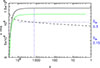 |
Fig. 3. Evolution of the velocity dispersion of models 102 and 103 (green) with redshift. The dashed line shows the fall of density due to dark matter mass loss. If the density is 0.3 at z = 1300, it is approximately 0.27 in the current epoch, which is within the observational uncertainties. |
3. Normalising to observations
The simplest bulk flow calculation is to average the velocities of all the particles in the final timestep. This is the PBH bulk velocity, however. A second caveat is that a very few particles have very high velocities due to close encounters and have found their way to very large radii. The smallness of this issue is shown in Figs. A.1 and A.2. The high-velocity tails are scarcely visible. It still is a reason to limit the inclusion radius of the bulk flow calculation.
Figure 4 shows the evolution of this bulk flow velocity field for our fiducial mass-losing run (Run 102) compared to a standard constant-mass control simulation. The cosmic matter density parameter, Ωm, is also shown by the dashed curve. In a standard cosmology, Ωm evolves purely due to cosmic expansion, but in our model, it also decreases as particles lose mass. The mass-loss rate in Run 102 was carefully calibrated so that Ωm declined by only 10% between the epoch of recombination (z ∼ 1100) and the present day (z = 0). This specific constraint was chosen to ensure that our model did not violate late-time cosmological probes, such as the luminosity distances of Type Ia supernovae or the growth of structure inferred from weak lensing, which tightly constrain the recent expansion history (Vincenzi et al. 2024). The quantitative results are summarised in Table 2. The bulk flow, calculated as the median velocity of all particles within spherical top-hat volumes, is shown for two representative scales.
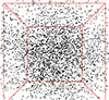 |
Fig. 4. Central part of run 104, timestep 99 in 3D. |
Bulk flow of particles.
The first row in Table 2 gives the three components of the bulk flow velocity, and the second row lists their uncertainty. The first column in the table gives the number of particles in the calculation. The third row shows the significance 1, 2, or 3σ of the bulk flow measurement. At large radii (median particle separation) and smaller radii (half that), the mass-losing model generates a bulk flow with an amplitude approximately twice that of the constant-mass model. This statistically significant enhancement arises because the early higher-density phase allows for greater initial velocity kicks, while the subsequent mass loss reduces the gravitational potential of large-scale structures, preventing these high velocities from being decelerated as strongly as in a standard cosmology. This result is in line with observational tensions, bringing the model predictions into much closer alignment with the high-amplitude flows of ∼400 km s−1 measured on scales > 100 h−1 Mpc (Watkins et al. 2023).
Table 2 demonstrates that the higher peculiar velocities are indeed attained by the models incorporating mass loss. These and all simulations reported here employed N = 256 000 particles within a cosmological volume, evolved using the gravitational N-body code of Mould & Hurley (2025). The number of adaptive timesteps required to reach the final state at z ∼ 0 ranged from 70 to 100.
To make a meaningful comparison with observations, however, we need to examine the bulk flow velocities of identified dark matter haloes, which serve as proxies for galaxies. A two-point correlation followed by a three-point correlation was used to find (proto)galaxies in the simulations. In practice, this meant finding galaxy pairs separated by the median radius divided by  1000, and then forming triangles from these galaxies, whose sides summed to less than the median radius divided by
  5000. This is a heuristic approach, and it should be compared with the more tested friends-of-friends algorithm.
Although the simulations are inherently scale-free, applying this galaxy finder suggests a physical scale4. When the particle velocities are set to be in km s−1, with G = 1 in the code, then M = v2 r means that a particle represents 108 M⊙ and a pixel of distance, r, of 0.5 pc. The conclusions below are independent of this normalization. When 100 DM particles are chosen to be the minimum to represent a galaxy, then that galaxy in the toy model is about 1010 M⊙. With these considerations in mind and cognizant of these limitations in the normalization, I present results for the bulk flows of identified haloes in Table 3. The row with the run number in Table 3 gives the number of galaxies found (18 in the case of run 111), the bulk flow velocity  (13 038 units in the case of run 111), and the starting redshift z0. The next row gives the bulk flow velocity components. The third row gives the 1σ uncertainties in the components.
Bulk flow of galaxies with more than 100 particles.
4. Bulk flow of galaxies
It is clear from these results and Fig. 5 that starting the halo formation from a high redshift rather than from linear perturbations at z ≈ 100 (t ≈ 17 Myr in a standard cosmology) is the primary driver of the high bulk flows. This presence of collapsed high-density objects at very early times is a natural property of PBHs. PBHs with masses M < 10−17 M⊙ would form from the collapse of large-amplitude primordial density fluctuations at redshifts z > 1010, acting as massive seeds for structure formation long before the baryonic Jeans mass would allow for conventional galaxy formation.
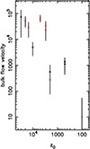 |
Fig. 5. Resultant bulk flow velocity increased with increasing initial redshift, z0. The solid symbols are taken from Table 3 and represent assemblies of dark matter with more than 100 particles. The open symbols are taken from the appendix and are unrestricted as to the number of particles. Simulations with mass loss are plotted in red. |
The PBH formation mechanisms, of which there are many, none of which has the status of a widely agreed model5, are not expected to make black holes of a single mass. It is therefore useful to consider which range of masses loses ∼1% per timestep of their mass, typical of the calculations here. This is shown in Fig. 6 for the Mosbech & Picker (2022) formula and for the redshift range (100, 10 000).
 |
Fig. 6. Percentage of DM required to produce an average 1% mass loss per timestep in one of the runs in Table 1. This takes only a 1% portion of the total DM to have this mass for m20, but 100% for m19.3. The steep slope arises from fractional mass-loss rates, 1/M dM/dt ∝ M−3. |
Various initial mass functions of PBHs are considered in the literature, but this is beyond the scope of the present work.
5. Discussion
Three matters seem well worth further consideration. First, why the bulk flow is affected by PBHs; second, how mass loss is accommodated in the Friedmann equation, and third, how these results should be followed up.
On primordial scales, Silk damping effectively erases baryonic density fluctuations below the photon diffusion scale (≈1013 M⊙) prior to recombination. Similarly, the free-streaming of certain dark matter candidates such as warm DM or hot DM smooths the density field on scales up to their respective free-streaming lengths (Sarkar et al. 2017). There is very little that can retard6 the acceleration of PBHs by their mutual gravitational interactions, however, and the hierarchical clustering and velocity growth of PBHs. As discrete and compact objects, their effective interaction cross section arises from their small geometric size. Consequently, processes such as dynamical friction, which depend on scattering off a sea of lighter background particles, are highly inefficient in an early Universe dominated by a population of PBHs with similar masses.
A very simple physical effect is therefore seen to be at work here. Either because the density at a redshift of about 103 is higher (Fig. 3) or because the period for gravitational interaction is longer, or both, the rms velocities of the haloes that will form galaxies are raised. This combination inevitably raises the velocity dispersion of the PBH population that will later seed galaxy formation. Although I concentrated on PBHs here, there are other macroscopic DM candidates that precede WIMPs in forming galaxy haloes. Axion miniclusters (Kolb & Tsachev 1996, Fairbairn, et al. 2017) begin their gravitational interactions right at the matter-radiation equality and would share the bulk-flow-raising properties of PBHs, but not their mass loss.
5.1. PBH cosmology
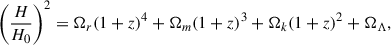
The option for Ωm to vary over some fraction of the lifetime of the Universe is readily accommodated in the Friedmann equation,
 (1)
(1)
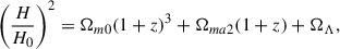
where H0 is the Hubble constant, and Ωr, Ωm, Ωk, and ΩΛ are the radiation and matter density, the curvature, and cosmological constant relative to the critical density. When the changing matter density is written as Ωm = Ωm0 + Ωm′(1 + z) by analogy with w and w′ in time-varying7 dark energy models and choose a flat Universe, Eq. (1) becomes
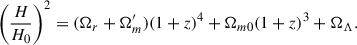 (2)
(2)
That is, ΩM′ is accommodated by an increasing radiation term Ωr by Ωm′. This is so, regardless of whether the evaporating PBH releases 100% radiation. This has the effect of delaying matter-radiation equality and requiring a correction to the Planck Collaboration VI (2020) value of the Hubble constant. To preserve the precisely measured angular scale of the sound horizon at last scattering, this change to the pre-recombination expansion history necessitates a compensatory increase in the expansion rate, H0, thereby helping to alleviate the Hubble tension. This effect is separate from the effect of the PBH ionisation time-bomb (Batten & Mould 2025). For instance, doubling the effective radiation energy density shifts the redshift of last scattering in the Recfast code (Seager et al. 2000) by δz = 13, which requires a compensatory H0 increase of approximately 1.5%.
Although it might appear that this model could be ruled out by next-generation supernova cosmology experiments achieving close to 1% precision in the comparison of Ωm derived from the CMB with that from z = 0 – 2 probes, it is not so simple. The model possesses sufficient flexibility; for instance, by manipulating the PBH initial mass function to favour higher-mass PBHs (which evaporate more slowly), or by postulating a WIMP half-life that ensures that decay is > 99% complete by z > 1100, we can engineer a scenario in which the mass loss effectively ceases before recombination, leaving the late-time expansion history virtually indistinguishable from ΛCDM.
To robustly verify these early Ωm′ simulations, higher-resolution runs with particle numbers of N > 107 would be desirable, so that galaxy-mass haloes are resolved by thousands of particles rather than hundreds, allowing for a more accurate treatment of the halo substructure and merger dynamics. A suite of N-body simulations for the ΛCDM power spectrum has been prepared for the Euclid mission (Rácz et al. 2025), extending to wavenumbers of k ∼ 140 h Mpc−1. All of them show the characteristic decline in power on large scales (small k) that differs from peculiar velocity surveys (Hoyle et al. 2000; Scargle et al. 2017). Simulations incorporating the PBH-seeded mass-losing dark matter mechanism, as outlined here, would be a valuable and timely addition to this effort.
Looking to the future, we expect that simulations will show that a million redshifts within z = 0.1 with rms distance uncertainties of 20% will measure a bulk flow to an accuracy of ±11 km s−1. These will be available when DR1 of DESI has been processed for peculiar velocities. These simulations also show that the radius of a bulk flow can be determined with precision8. So there is a reasonable expectation that power on large scales can be well measured.
5.2. The Friedmann equation as a fitting function
With the discovery of dark energy, the Friedmann equation morphed from an equation relating matter and radiation density to the General Relativity curvature of space to a fitting function. Figure 7 shows the Planck cosmology fit to the Dark Energy Survey OzDES supernova distance moduli (DES Collaboration 2024). This can be compared with the distance moduli without dark energy (the red line). The green line shows Eq. (3),
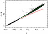 |
Fig. 7. Currently leading supernova cosmology Hubble diagram of DES Collaboration (2024; distance modulus vs. redshift). The open circles show outliers that were not used in the fit. The solid line shows the Planck cosmology fit, the red curve shows the same equation without dark energy, and the green curve shows Eq. (3) with the optimum value of Ωma2. |
 (3)
(3)
which defines Ωm = Ωm0 + Ωma2/(1 + z)2, which simply uses a different functional form to express mass loss. It is a good fit, but mass loss cannot replace dark energy. It can modify the distance moduli by 0.075 mag, which is the difference been 10% more or less dark energy at z = 1. The Planck power spectrum constraint on curvature has been acknowledged by choosing Ωma2 rather than Ωma. It will be interesting to see whether Eq. (3) can be fitted to the millions of redshifts of DESI as well as to the dynamic dark energy w0-wa cosmology (Roy Choudhury 2025; DESI Collaboration 2022). It remains to be determined whether a prescription exists for a PBH IMF that would approximate this fit.
6. Conclusions
To provide more power at large scales, we may not need to depart from the ΛCDM paradigm, assuming PBHs can be considered cold dark matter. Just as the DESI Collaboration (2025) has embraced a time-varying equation of state, parametrised by w0 and wa, what is being trialled here with PBHs is a variable ΩmΛCDM cosmology. Until we better understand the physics of DM, this may be the closest we can approach to a standard model that can fit bulk flow constraints. These calculations have focussed on PBHs, in part because they involve no new physics, but they apply to decaying DM generally. Cosmological simulations are a mature science, and we caution about results from a toy model until they have been explored further with codes for dark matter and gas plus dark matter. In the cosmology fitted to the DESI data, the equation-of-state parameter is w(z) ≡ w0 + wa z/(1 + z). A PBH mass-loss parameter should be investigated as a physical alternative to wa. Finally, simulations starting at or before matter-radiation equality should be explored for axion miniclusters because these might also produce CMB dipole-sized bulk flows.
Acknowledgments
The ARC Centre of Excellence for Dark Matter Particle Physics is funded by the Australian Research Council through grant CE200100008. Simulations were carried out on Swinburne University’s Ozstar & Ngarrgu Tindebeek supercomputers, the latter named by Wurundjeri elders and translating as “Knowledge of the Void” in the local Woiwurrung language. I would like to thank the organizers of CosmicFlows 2025 for a conference that informed and inspired this paper. I am grateful to Darren Croton for helpful advice and also to the journal editor and referee. Google Gemini Pro 2.5.0 helped to render this paper more readable. Thanks to Tamara Davis for supplying the OzDES supernova data. Code availability Suitable n-body codes are reviewed by Bertschinger (1998), and thanks to Michael Blanton for the visualization code P3D.
References
- Aaronson, M., & Olszewski, E. W. 1988, IAUS, 130, 185 [Google Scholar]
- Alonso-Monsalve, E., & Kaiser, D. 2023, PRL, 132, 231402 [Google Scholar]
- Batten, A., & Mould, J. 2025, MNRAS, submitted [Google Scholar]
- Bertschinger, E. 1998, ARAA, 36, 599 [Google Scholar]
- Böhringer, H., Chon, G., Trümper, J., et al. 2025, A&A, 695, A59 [NASA ADS] [CrossRef] [EDP Sciences] [Google Scholar]
- Bouillot, V., Alimi, J., Rasera, Y., & Füzfa, A. 2014, Front. Fund. Phys. Phys. Education Res., 145, 89 [Google Scholar]
- Colless, M. 2024, IAUGA, 32, 1950 [Google Scholar]
- Courtois, H., Mould, J., Hollinger, A. M., et al. 2025, A&A, 701, A187 [NASA ADS] [CrossRef] [EDP Sciences] [Google Scholar]
- Dekel, A. 1993, ASPC, 51, 194 [Google Scholar]
- DES Collaboration (Abbott, T. M. C., et al.) 2024, ApJ, 973, L14 [NASA ADS] [CrossRef] [Google Scholar]
- DESI Collaboration (Abareshi, B., et al.) 2022, AJ, 164, 207 [NASA ADS] [CrossRef] [Google Scholar]
- DESI Collaboration (Adame, A. G., et al.) 2025, JCAP, 7, 28 [Google Scholar]
- Di Valentino, E., Perivolaropoulos, L., & Said, J. 2024, Universe, 10, 184 [Google Scholar]
- Fairbairn, M., Marsh, D., & Quevillon, J. 1996, PRL, 119, 021101 [Google Scholar]
- Hoyle, F., Szapudi, I., & Baugh, C. 2000, ApJ, 317, L51 [Google Scholar]
- Hudson, M., Smith, R., Lucey, J., & Branchini, E. 2004, MNRAS, 352, 61 [Google Scholar]
- Inman, D., & Ali-Haïmoud, Y. 2019, Phys. Rev. D, 100, 083528 [NASA ADS] [CrossRef] [Google Scholar]
- Kolb, E., & Tsachev, I. 1996, ApJ, 460, L25 [Google Scholar]
- Lauer, T., & Postman, M. 1994, ApJ, 425, 418 [Google Scholar]
- Li, B., Tanga, C.-Y., Huanga, Z.-R., & Liu, L.-H. 2025, JCAP, 12, 8 [Google Scholar]
- Mosbech, M., & Picker, G. 2022, SciPost, 13, 100 [Google Scholar]
- Mould, J. 2025, ApJ, 984, 59 [Google Scholar]
- Mould, J., & Hurley, J. 2025, arXiv e-prints [arxiv:2509.02165] [Google Scholar]
- Niikura, H., Takada, M., Yasuda, N., et al. 2019, Nat. Astron., 3, 524 [NASA ADS] [CrossRef] [Google Scholar]
- Pérez de los Heros, C. 2020, Symmetry, 12, 1648 [Google Scholar]
- Planck Collaboration VI. 2020, A&A, 641, A6 [NASA ADS] [CrossRef] [EDP Sciences] [Google Scholar]
- Poulin, V., Desgourges, J., & Serpico, P. 2017, JCAP, 3, 43 [Google Scholar]
- Rácz, G., Breton, M.-A., Fiorini, B., et al. 2025, A&A, 695, 232 [Google Scholar]
- Roy Choudhury, S. 2025, ApJ, 986, L31 [Google Scholar]
- Sarkar, A., Sethi, K., & Das, S. 2017, JCAP, 7, 12 [Google Scholar]
- Scargle, J., Way, M., & Gazis, P. 2017, ApJ, 839, 40 [Google Scholar]
- Scrimgeour, M., Davis, T. M., Blake, C., et al. 2016, MNRAS, 455, 386 [Google Scholar]
- Seager, S., Sasselov, D., & Scott, D. 2000, ApJS, 128, 407 [NASA ADS] [CrossRef] [Google Scholar]
- Secrest, N. 2025, RSPTA, 38340027 [Google Scholar]
- Taylor, E. N., et al. 2023, ESO Messenger, 190, 46 [Google Scholar]
- Tsagas, C., Perivolaropoulos, L., & Asvesta, K. 2025, arXiv e-prints [arXiv:2510.05340] [Google Scholar]
- Tully, R. B. 1989, ASSL, 151, 41 [Google Scholar]
- Vincenzi, M., Brout, D., Armstrong, P., et al. 2024, ApJ, 975, 86 [NASA ADS] [CrossRef] [Google Scholar]
- Watkins, R., & Feldman, H. 2025, arXiv e-prints [arXiv:2512.03168] [Google Scholar]
- Watkins, R., Allen, T., Bradford, C. J., et al. 2023, MNRAS, 524, 1885 [NASA ADS] [CrossRef] [Google Scholar]
- Whitford, A., Howlett, C., & Davis, T. 2023, MNRAS, 526, 3051 [NASA ADS] [CrossRef] [Google Scholar]
An exception and a partial exception is work by Scrimgeour et al. (2016) and Courtois et al. (2025).
Reviewed by Di Valentino et al. (2024).
Before recombination, the gas would be fully coupled to the radiation and not to the dark matter. Even up until z ∼100, an order-unity fraction of the baryons would be coupled to the CMB radiation. In general, the gas is significantly hotter than the dark matter and can also have a significant net relative velocity on small scales.
The most likely mass for PBH DM lies in the asteroid window, which has not been reached by microlensing. Applying a galaxy finder to unite DM particles into haloes associates a small number of neighbour particles to represent a galaxy of mass 108 to 1010 M⊙. They do not become 108 M⊙ particles, however. The simulations are scale-free in mass, length, and time, and the actual particle mass is not specified.
The detection of PBHs is also a matter of debate. In the mass range from stars to asteroids, microlensing observers have tended to publish both candidate events and PBH upper limits (e.g. Niikura et al. 2019 and Li et al. 2025).
For a PBH of mass 10−10 M⊙ at z = 104, the stopping distance due to ρv2 pressure is an extraordinary 1050/m10 cm. For dynamical friction, it is approximately 1035v1004/m10 cm, where v100 is the velocity in units of 100 km s−1. The radiation pressure exceeds the gas pressure by a factor of 109, but does not change the situation.
Recent work by the DES and DESI collaborations has favoured w0 and wa over w and w′.
Peculiar velocities must be corrected for Malmquist bias, if the systematic errors are not to exceed the random errors calculated here. This requires attention to the detail of sample selection effects.
Appendix A: Simulation details
A.1. Boundary conditions
The n-body code used here was written to investigate the formation of dark clusters from PBH. The particles expanded into a vacuum. The same code (Mould & Hurley 2025) is used here. Normally, cosmological simulations have periodic boundary conitions to preserve homogeneity and isotropy, in contrast to the present simulations which deviate from homogeneity at the distances of the furthest particles. This was investigated by rerunning simulation 103 with reflective boundary conditions, in which the simulation is contained in a box which expands with the scale factor. Particles penetrating the box have their velocities reflected. The modified run 103 differed from the original rms velocity by 5%.
A.2. Additional simulations
Simulations in which fewer than 100 particles per galaxy were available are summarised here. The final velocity distribution functions of runs 104-107 are shown in Figs. A.1 and A.2.
Bulk flow of galaxies (< 100 particles).
A.3. Dynamic dark energy
The current DESI cosmology is compared with mass losing DM in Fig. A.3.
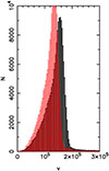 |
Fig. A.1. Velocity distribution functions for run 104 and run 105 (red). |
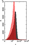 |
Fig. A.2. Velocity distribution functions for run 106 and run 107 (red). |
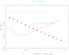 |
Fig. A.3. Remarkable small difference between galaxy luminosity distances due to dynamic dark energy. Distances are ratioed to static dark energy (the green line). The red curve is the cosmology of Abdul Karim et al. (2025). Its turnaround is due to matter domination for z > 1. The points are for DM mass loss with Ωm′ = 0.015. They do not turn around because Ωm′ is still effective at z > 1. That could be remedied by suitable choice of a PBH IMF. |
All Tables
All Figures
|
Fig. 1. Temperature evolution of low-mass PBHs vs. cosmic temperature. In the radiation-dominated era, PBHs of mass 10−23 M⊙ (denoted m23) and higher, if they form, do so on the green diagonal line and evolve with little mass loss until Ṁ is of the same order as M, at which point they rapidly heat and evaporate. Kelvin units are used at the top and right borders. PBHs change their evolutionary rate as T ∼ M−1, from radiation (solid line), to matter (dashed line), to dark-energy dominated (dotted line). The t8 line marks the start of galaxy formation. The three dotted vertical lines are from left to right the QCD transition at 220 MeV, the surface of last scattering of the CMB, and the temperature today, 2.7 K. |
| In the text | |
|
Fig. 2. Enlargement of Fig. 1 for z < 105. Redshift log(1+z) is denoted by the numbers towards the top. The CMB is shown by the vertical dotted line, and 108 years is shown by the vertical dashed green line. |
| In the text | |
|
Fig. 3. Evolution of the velocity dispersion of models 102 and 103 (green) with redshift. The dashed line shows the fall of density due to dark matter mass loss. If the density is 0.3 at z = 1300, it is approximately 0.27 in the current epoch, which is within the observational uncertainties. |
| In the text | |
|
Fig. 4. Central part of run 104, timestep 99 in 3D. |
| In the text | |
|
Fig. 5. Resultant bulk flow velocity increased with increasing initial redshift, z0. The solid symbols are taken from Table 3 and represent assemblies of dark matter with more than 100 particles. The open symbols are taken from the appendix and are unrestricted as to the number of particles. Simulations with mass loss are plotted in red. |
| In the text | |
|
Fig. 6. Percentage of DM required to produce an average 1% mass loss per timestep in one of the runs in Table 1. This takes only a 1% portion of the total DM to have this mass for m20, but 100% for m19.3. The steep slope arises from fractional mass-loss rates, 1/M dM/dt ∝ M−3. |
| In the text | |
|
Fig. 7. Currently leading supernova cosmology Hubble diagram of DES Collaboration (2024; distance modulus vs. redshift). The open circles show outliers that were not used in the fit. The solid line shows the Planck cosmology fit, the red curve shows the same equation without dark energy, and the green curve shows Eq. (3) with the optimum value of Ωma2. |
| In the text | |
|
Fig. A.1. Velocity distribution functions for run 104 and run 105 (red). |
| In the text | |
|
Fig. A.2. Velocity distribution functions for run 106 and run 107 (red). |
| In the text | |
|
Fig. A.3. Remarkable small difference between galaxy luminosity distances due to dynamic dark energy. Distances are ratioed to static dark energy (the green line). The red curve is the cosmology of Abdul Karim et al. (2025). Its turnaround is due to matter domination for z > 1. The points are for DM mass loss with Ωm′ = 0.015. They do not turn around because Ωm′ is still effective at z > 1. That could be remedied by suitable choice of a PBH IMF. |
| In the text | |
Current usage metrics show cumulative count of Article Views (full-text article views including HTML views, PDF and ePub downloads, according to the available data) and Abstracts Views on Vision4Press platform.
Data correspond to usage on the plateform after 2015. The current usage metrics is available 48-96 hours after online publication and is updated daily on week days.
Initial download of the metrics may take a while.