© The Authors 2026

1. Introduction

One of the most fundamental and basic properties of galaxies is the rate at which new stars form, the star formation rate (SFR). The SFR is sensitive to the interplay between the gas inflow and outflow rates of galaxies, and the efficiency at which this gas is converted into stars (e.g., Bouché et al. 2010; Lilly et al. 2013; Behroozi et al. 2019). The SFR can fluctuate on different timescales (e.g., Sparre et al. 2015; Iyer et al. 2020; Flores Velázquez et al. 2021), which range from dynamical timescales of molecular clouds (some dozens of million years) through galaxy merger timescales (∼100 Myr) to long (Gyr-scale) coherences in accretion rates (e.g., Matthee & Schaye 2019; Wang & Lilly 2020; Tacchella et al. 2020; Wan et al. 2025). Observationally, SFRs can be measured using various diagnostics (e.g., Kennicutt & Evans 2012; De Looze et al. 2014; Davies et al. 2019) that are either based on the light from massive short-lived stars (e.g., the rest-frame UV), or processed radiation (e.g., nebular lines in HII regions or dust emission). Each of these diagnostics probes different timescales of star formation and is differently affected by dust attenuation.

At high redshifts (z > 3), the rest-frame UV emission used to be the most sensitive SFR indicator that could be measured for large galaxy samples. It traces star formation on timescales of t ∼ 100 Myr (e.g., Bouwens et al. 2015). However, dust corrections in the rest-frame UV are significant, with potentially up to 50% of the cosmic SFR density (ρ_SFR) at z ∼ 5 being obscured by dust (e.g., Zavala et al. 2021; Sun et al. 2025). This emphasizes the great importance of alternative SFR indicators that are less sensitive to dust attenuation, such as the Hα emission. The Hα photons are emitted in the rest-frame optical (λ = 6564 Å), where dust corrections are smaller than in the rest-frame UV due to the negative slope of the dust attenuation curve (however, we caution that there is growing evidence of flatter attenuation curves at fixed A_V or stellar mass at high redshifts compared to the local Universe; e.g., Shivaei et al. 2025; Fisher et al. 2025). The luminosity of the Hα line is directly proportional to the luminosity of ionizing photons that are predominantly emitted by very young stellar populations, making Hα sensitive to star formation on shorter timescales (t ∼ 10 Myr; e.g., Leitherer et al. 1999). As the James Webb Space Telescope (JWST) can now measure the distribution of Hα luminosities out to z ∼ 7 based on spectroscopy and narrow-band imaging (e.g., Clarke et al. 2024; Pirie et al. 2025; Covelo-Paz et al. 2025; Fu et al. 2025), it is timely to reassess the role of the Hα emission as a tracer of the SFR.

The conversion factor between the Hα luminosity¹ and the SFR primarily depends on assumptions on the properties of stellar populations, in particular, the star formation history (SFH), the initial mass function (IMF), binarity, and stellar metallicity (e.g., Wilkins et al. 2019). The SFH and IMF are relevant because the ionizing photon emissivity from a single stellar population drops sharply after a few million years when massive short-lived O stars leave the main sequence. Binary interactions can extend these ionizing lifetimes (Götberg et al. 2017) and smooth the otherwise steep drop-off after a few million years. At fixed stellar mass and age, the metallicity affects the effective temperature of stellar atmospheres due to line blanketing effects that also affect the ionizing luminosity.

The classical SFR(Hα) calibration proposed by Kennicutt (1998) (see also Kennicutt & Evans 2012) assumes a constant SFH over t = 100 Myr and solar metallicity, based on the typical conditions in galaxies in the low-redshift Universe. However, various spectroscopic observations of galaxies at high redshifts suggest that their SFHs are bursty (e.g., Asada et al. 2024; Endsley et al. 2024; Cole et al. 2025; Carvajal-Bohorquez et al. 2025). Further, given the gas-phase oxygen abundances are typically measured to be ∼10% solar (Curti et al. 2024; Scholte et al. 2025), and early galaxies are expected to be α-enhanced due to the rapid formation timescales (e.g., Chruślińska et al. 2024), the iron-peak element abundances are likely to be low. This implies hotter stars and a more efficient Hα photon production at a fixed SFR (e.g., Theios et al. 2019) than at low redshift.

The aim of this paper is to revisit the classical SFR(Hα) calibrations to predict the SFRs of galaxies at high redshift (z ≳ 3). Instead of using idealistic models with constant SFHs and fixed stellar metallicities, we use simulated galaxies and their modeled Hα luminosities from the SPHINX cosmological radiation-hydrodynamical simulation (Rosdahl et al. 2018; Katz et al. 2023). These cosmological simulations self-consistently model SFHs and metal enrichment processes and are calibrated to match various observables at high redshifts (z ∼ 6). The simulated volume matches the typical volumes of deep JWST surveys well, which enables a high resolution that can capture SFR variations on short timescales (t ∼ 1 Myr) and approximate the distribution of gas in the interstellar medium relevant for radiative transfer effects.

In Sect. 2 we briefly describe the SPHINX simulations and explain how the Hα luminosities are derived. In Sect. 3 we present a set of simulation-inferred SFR(Hα) calibrations that predict the SFRs of SPHINX galaxies with very little error. Finally, we discuss the implications of our work in Sect. 4 and summarize in Sect. 5.

2. Methods

We used the simulated galaxy data from SPHINX, a suite of cosmological radiation-hydrodynamic simulations (Rosdahl et al. 2018). SPHINX leverages the adaptive mesh refinement code RAMSES-RT (Rosdahl et al. 2013; Teyssier 2002) to simulate tens of thousands of galaxies in the epoch of reionization. The ISM is resolved down to 76 comoving parsec, corresponding to a physical resolution of 11 pc at z = 6. The dark matter halos are resolved down to the atomic cooling threshold (M_vir ≈ 3 × 10⁷ M_⊙). Hydrodynamics, nonequilibrium thermochemistry, and radiative transfer of Lyman-continuum radiation (LyC; λ < 912 Å) are performed self-consistently on the fly, with subgrid implementations for gas cooling, star formation, metal enrichment, and feedback. The on-the-fly radiative emission and propagation of LyC photons make SPHINX an excellent model for accurately predicting how Hα emission traces star formation in the simulated galaxies.

Our analysis is based on the data from the SPHINX²⁰ Public Data Release, Version 1 (SPDRv1; Katz et al. 2023). SPHINX²⁰ is the largest simulation of the SPHINX suite, with a periodic box with a volume of (20 cMpc)³ simulated down to a redshift of z = 4.64 (Rosdahl et al. 2022). SPHINX²⁰ uses the BPASS V2.2 stellar population synthesis (SPS) model (Stanway & Eldridge 2018), which adopts a Kroupa (2001) IMF with an upper mass cutoff of 100 M_⊙ and a slope of −1.3 from 0.1 to 0.5 M_⊙ and −2.35 from 0.5 to 100 M_⊙. The intrinsic Balmer line luminosities were generated by interpolating the CLOUDY v17.03 models (Ferland et al. 2017) for gas cells that host stellar particles with unresolved Stromgren spheres, or by using the nonequilibrium ionizing fractions from the simulation otherwise. For each halo, the total intrinsic line emission is then the sum of the line luminosities of all gas cells within the virial radius of the halo. The equivalent widths were calculated by taking the stellar and nebular continuum emission into account, generated as detailed in Katz et al. (2023).

We post-processed the line and continuum radiation, subject to absorption and scattering by dust, using the radiative transfer code RASCAS (Michel-Dansac et al. 2020). Dust was assigned to the gas cells using the Small Magellanic Cloud (SMC) dust model from Laursen et al. (2009). We note that the dust attenuation curve at high redshifts likely has a steeper slope than the SMC slope (e.g., Shivaei et al. 2025; Markov et al. 2025), possibly due to changes in the dust grain properties. Next, 200 000 photon packets were probabilistically distributed to the gas cells, with the initial wavelengths placed at the line centers, thermally broadened, and shifted according to the bulk velocity of the cell. Likewise, 200 000 photon packets were probabilistically distributed to the star particles (gas cells) based on the luminosities of the stellar (nebular) continuum at the line centers. The observed line luminosities and equivalent widths were then obtained by computing the escape fractions of each component (for details, see Katz et al. 2023).

Limitations in computation time and data storage mean that SPDRv1 only includes SPHINX²⁰ galaxies with SFR₁₀ ≥ 0.3 M_⊙ yr⁻¹, where SFR₁₀ is the SFR averaged over t = 10 Myr. This excludes objects that are likely too faint to be observed with JWST (Katz et al. 2023), unless lensing is considered (e.g., Bezanson et al. 2024; Naidu et al. 2024). However, an SFR cut also leads to an incompleteness in the SFR–L_Hα relation at low luminosities, which can bias our results. We therefore limited our selection of galaxies from SPDRv1 to those with an observed Hα luminosity ($L_{\mathrm{H}\alpha }^{\mathrm{obs}}$) greater than $L_{\mathrm{H}\alpha }^{\mathrm{obs}}=1.8\times {10}^{41}$ erg s⁻¹ (we used the simulation-based luminosities calculated as described above). This value was motivated by the recent Hα LF measurements from JWST Near Infrared Camera (NIRCam)/grism, which reach similar luminosities at the faint end (e.g., Fu et al. 2025). Crucially, this selection yields a complete Hα-emitter sample, which we checked by running RASCAS on all SPHINX²⁰ halos whose intrinsic Hα luminosity ($L_{\mathrm{H}\alpha }^{\mathrm{int}}$) exceeded the luminosity cut. We also tried $L_{\mathrm{H}\alpha }^{\mathrm{obs}}>1.0\times {10}^{41}$ erg s⁻¹ and $L_{\mathrm{H}\alpha }^{\mathrm{obs}}>3.0\times {10}^{41}$ erg s⁻¹ cuts, but found little impact on our results. With this additional luminosity cut, our final sample comprised N = 63, 66, 48, 36, 22, 17, and 13 galaxies at z = 4.64, 5, 6, 7, 8, 9, and 10, respectively, with a total of N = 265 galaxies.

The SN feedback model in SPHINX is calibrated to match the UV luminosity function (UVLF) at z = 6 (see Appendix C in Rosdahl et al. 2018). A possible caveat is that the stellar mass-halo mass relation in SPHINX is 0.5–1.0 dex higher than predicted by the Behroozi et al. (2019) model, for example, which matches a broad array of observational data, including stellar mass functions at z = 0–4 and median UV-stellar mass relations at z = 4–8 (see Fig. 4 in Katz et al. 2023). Furthermore, the stellar mass function (SMF) in SPHINX is significantly overestimated compared to the SMF inferred from the JWST/NIRCam observations at z = 5–6 (Weibel et al. 2024). If the stellar masses of SPHINX galaxies are overestimated, the SFRs are probably also overestimated on average. This implies that the amount of dust in the simulation is probably higher than in the real Universe in order to match the UVLF. The excess of dust would then explain the fact that SPHINX predicts lower Hα and [O III] luminosities at fixed stellar mass than those measured by JWST (e.g., Covelo-Paz et al. 2025; Meyer et al. 2024). Although the possibility of SPHINX galaxies having too much dust does not affect our main results as they are based on the intrinsic Hα properties (Sect. 3), it will become important later for understanding the errors in the SFR(Hα) calibrations that use the observed Hα (Sect. 4).

3. Results

In this section, we investigate the intrinsic (i.e., without taking dust attenuation into account) SFR–L_Hα relation in the SPHINX²⁰ cosmological simulation. We compare this relation to the SFR(Hα) calibrations from the literature and study the effect of the variations in the physical properties of individual galaxies (metallicity, stellar age, etc.) on the accuracy of the predicted SFRs. Based on this analysis, we develop a set of new SFR(Hα) calibrations that minimize the error in Hα-derived SFRs at high redshift.

Unless otherwise specified, we used the SFRs averaged over the last t = 10 Myr of the SFH. This choice was motivated by the fact that nebular emission lines such as Hα trace stars with lifetimes of t ∼ 3–10 Myr (e.g., Kennicutt & Evans 2012). This is further supported by the simulation itself, where the correlation coefficient between the SFR and $L_{\mathrm{H}\alpha }^{\mathrm{int}}$ peaks between 4 Myr ≲ t ≲ 12 Myr (r ≈ 0.95–0.98; see Appendix A).

3.1. The SFR–L_Hα relation in SPHINX

Figure 1 shows the intrinsic SFR–L_Hα relation for the galaxy sample selected from the SPHINX²⁰ simulation as described in Sect. 2. In the same figure, we show different SFR(Hα) calibrations proposed in the literature. These include the original K98 calibration (C_Hα = −41.1), the K98 calibration converted into the Kroupa IMF (Kroupa 2001; C_Hα = −41.3), and two calibrations from Theios et al. (2019, hereafter T19) calculated for a Kroupa-type IMF and solar metallicity (C_Hα = −41.35), and the same IMF, but subsolar metallicity (Z_* = 0.1 Z_⊙; C_Hα = −41.64), respectively. Here, C_Hα is the conversion factor between $L_{\mathrm{H}\alpha }^{\mathrm{int}}$ and SFR, defined as follows:

$$\begin{array}{c}\hfill {log}_{10}\left[\frac{\mathrm{SFR}}{M_{\odot }{\mathrm{yr}}^{-1}}\right]={log}_{10}\left[\frac{L_{\mathrm{H}\alpha }^{\mathrm{int}}}{\mathrm{erg}{\mathrm{s}}^{-1}}\right]+C_{\mathrm{H}\alpha }.\end{array}$$(1)

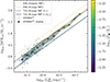Fig. 1. Intrinsic SFR–LHα relation in the SPHINX20 cosmological simulation, color-coded by the stellar metallicity. The SFR values are averaged over t = 10 Myr, i.e., the typical lifetime of stars traced by Hα. The diamonds show the median SFR in the bins of $L_{\mathrm{H}\alpha }^{\mathrm{int}}$, with the error bars showing the standard error on the median. The shaded region indicates the 68% (1σ) confidence interval. The diagonal lines show the SFR(Hα) calibrations from the literature, i.e. (top to bottom), the original K98 calibration, the K98 calibration converted into the Kroupa IMF, and two calibrations from T19 calculated for the Kroupa IMF and two different metallicities (Z* = Z⊙ and Z* = 0.1 Z⊙, respectively).

Figure 1 reveals that a constant C_Hα cannot provide an accurate estimate of the SFRs of SPHINX galaxies across the full $L_{\mathrm{H}\alpha }^{\mathrm{int}}$ range. Specifically, the T19 calibration that assumes Z_* = Z_⊙ (the dashed blue line in Fig. 1) matches the median SFR–L_Hα relation in SPHINX at high luminosities well (${log}_{10}(L_{\mathrm{H}\alpha }^{\mathrm{int}}/\mathrm{erg}{\mathrm{s}}^{-1})\gtrsim 42.2$). In contrast, the same SFR(Hα) calibration at low luminosities (${log}_{10}(L_{\mathrm{H}\alpha }^{\mathrm{int}}/\mathrm{erg}{\mathrm{s}}^{-1})\lesssim 42.2$) overestimates the SFRs by ≈0.1–0.2 dex. Decreasing C_Hα would result in a better match at low luminosities, but the SFRs at high luminosities would then be underestimated.

We note that the median SFR–L_Hα relation in SPHINX at low luminosities lies between the two T19 calibrations that differ only in the assumption on metallicity (Z_* = 0.1 Z_⊙ vs. Z_* = Z_⊙; indicated by the solid and dashed blue lines in Fig. 1, respectively). Motivated by this result, we tested whether the variations in metallicity might be a key factor driving the evolution of the median SFR–L_Hα relation in SPHINX. We split our sample into low- and high-$L_{\mathrm{H}\alpha }^{\mathrm{int}}$ groups (${log}_{10}(L_{\mathrm{H}\alpha }^{\mathrm{int}}/\mathrm{erg}{\mathrm{s}}^{-1})<42.2$ and ${log}_{10}(L_{\mathrm{H}\alpha }^{\mathrm{int}}/\mathrm{erg}{\mathrm{s}}^{-1})>42.2$, respectively), and calculated the median stellar metallicity² in each group. We obtained Z_* = 0.06 Z_⊙ and Z_* = 0.33 Z_⊙ in the low- and high-$L_{\mathrm{H}\alpha }^{\mathrm{int}}$ groups, respectively. In other words, brighter galaxies are more metal rich on average, which reflects the mass-metallicity relation (MZR) in SPHINX (for a discussion, see Katz et al. 2023), and likely causes an upturn of the median SFR–L_Hα relation at high luminosities (see also Fig. 1, where the markers are color-coded by metallicity).

Figure 1 further demonstrates that the original K98 calibration (indicated by the dotted orange line) overestimates the SFRs by ≈0.3–0.5 dex compared to SPHINX. One of the main reasons for this discrepancy is the difference in the IMFs: K98 uses the Salpeter (1955) IMF, whereas SPHINX uses a Kroupa-type IMF. After rescaling to the Kroupa IMF, the K98 calibration still predicts ≈0.1–0.3 dex higher SFRs than the simulation (the dashed orange line in Fig. 1). This difference cannot be eliminated even when using the T19 calibration, which, unlike the K98 calibration, assumes the same stellar population synthesis model as SPHINX (i.e., BPASS V2.2; the dashed blue line in Fig. 1). Therefore, the only way to fully reconcile the K98 calibration and the simulation data is to assume a subsolar metallicity, for some galaxies as low as Z_* = 0.1 Z_⊙ (the solid blue line in Fig. 1). As discussed in the introduction, a subsolar metallicity like this agrees well with the current estimates of the gas-phase metallicity and also with the direct estimates of stellar metallicities of galaxies at z ∼ 2 − 3 (Steidel et al. 2016; Cullen et al. 2019), although we caution that these were derived assuming constant SFHs, which might impact the results (Matthee et al. 2022).

Figure 1 also reveals that the SFR–L_Hα relation in SPHINX exhibits significant scatter around the median relation (hereafter, σ_SFR). In particular, we find that σ_SFR decreases from σ_SFR ≈ 0.17 dex at ${log}_{10}(L_{\mathrm{H}\alpha }^{\mathrm{int}}/\mathrm{erg}{\mathrm{s}}^{-1})=41.3$ to σ_SFR ≈ 0.04 dex at 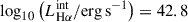${log}_{10}(L_{\mathrm{H}\alpha }^{\mathrm{int}}/\mathrm{erg}{\mathrm{s}}^{-1})=42.8$ and has a median σ_SFR = 0.11 dex. This scatter is neglected by the existing SFR(Hα) calibrations, leading to errors in the predicted SFRs of individual galaxies. To quantify this effect, we introduced the SFR bias factor, defined as the ratio of the SFR predicted from Hα to the true SFR directly tracked by the simulation: Δ_SFR ≡ SFR(Hα)/SFR₁₀. We used the T19 calibration that assumes Z_* = Z_⊙ to calculate SFR(Hα) as this calibration provides the best match to the SPHINX data (see Fig. 1). We note that using a different calibration would only change Δ_SFR by a constant factor (in logarithmic scale) without affecting any trends observed between Δ_SFR and the physical properties of SPHINX galaxies.

We found that Δ_SFR decreases with stellar metallicity (r = −0.51, p < 10⁻⁶; Fig. 2, top panel), in agreement with our earlier analysis of the median SFR–L_Hα relation in SPHINX. However, we also report a significant scatter in Δ_SFR at fixed Z_*: σ ≈ 0.09 dex. This indicates that metallicity alone does not cause the variations in the SFRs of SPHINX galaxies with respect to the SFRs predicted from Hα. In particular, we find that Δ_SFR shows a negative correlation with stellar age (r = −0.59, p < 10⁻⁶; Fig. 2, bottom panel), with an average scatter of σ ≈ 0.07 dex. Notably, galaxies with young stellar populations (t_age ≲ 5 Myr) exhibit high Δ_SFR (≈0.1–0.4 dex). Even when we used the best-fit SFR(Hα) calibration in the form of Eq. (1) (C_Hα = −41.45), Δ_SFR still reached ≈0.3 dex at t_age ≈ 2–3 Myr. This bias can be explained by the fact that the existing SFR(Hα) calibrations assumed constant star formation over a long timescale (typically t = 100 Myr or t = 1 Gyr; e.g., Hao et al. 2011). This assumption breaks down in the simulation, where galaxies exhibit very bursty and stochastic SFHs (Katz et al. 2023).

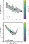Fig. 2. SFR bias factor (ΔSFR ≡ SFR(Hα)/SFR10) as a function of stellar metallicity (top) and age (bottom) in SPHINX, color-coded by EWHα. The SFR(Hα) values are calculated using the T19 calibration (Z* = Z⊙). The diamonds show the running median, with the error bars indicating the standard error on the median. The shaded region indicates the 68% (1σ) confidence interval.

We also examined the relation between Δ_SFR and stellar mass and found a negative correlation (r = −0.44, p < 10⁻⁶), likely driven by the positive scaling of stellar mass with metallicity (see Katz et al. 2023 for the discussion of the MZR in SPHINX). Finally, we investigated the dependence of Δ_SFR on the escape fraction of ionizing radiation (f_esc) and found a nearly flat trend (r = −0.21, p = 0.0009). This result is expected because the strength of nebular emission lines is inversely proportional to the escape fraction of ionizing photons, ∝(1 − f_esc), and SPHINX galaxies have low f_esc (f_esc ≲ 1%) on average. This agrees with high-redshift observations, where f_esc is also estimated to be low (< 10%; e.g., Mascia et al. 2024).

3.2. Simulation-informed SFR(Hα) calibrations

Using the insights gained from our analysis of the SFR–L_Hα relation in SPHINX, we discuss possible improvements to the existing SFR(Hα) calibrations that take the form of Eq. (1). For example, stellar metallicity might be a useful parameter to include in the calibration to reduce the error in the predicted SFR (see Fig. 2). However, measuring stellar metallicity is difficult in practice, and we therefore only used quantities that can be measured robustly from galaxy spectra. Specifically, we ran an ordinary least-squares (OLS) model similar to Eq. (1), but allowing the ${log}_{10}(L_{\mathrm{H}\alpha }^{\mathrm{int}}/\mathrm{erg}{\mathrm{s}}^{-1})$ coefficient to vary. We used randomly selected 80% of the sample to train the model and the remaining 20% to validate its performance. The resulting SFR(Hα) calibration can be written as follows:

$$\begin{array}{cc}\hfill {log}_{10}\left[\frac{\mathrm{SFR}}{M_{\odot }{\mathrm{yr}}^{-1}}\right]& ={log}_{10}\left[\frac{L_{\mathrm{H}\alpha }^{\mathrm{int}}}{\mathrm{erg}{\mathrm{s}}^{-1}}\right]-41.45\hfill \\ \hfill & +0.06({log}_{10}\left[\frac{L_{\mathrm{H}\alpha }^{\mathrm{int}}}{\mathrm{erg}{\mathrm{s}}^{-1}}\right]-41.90),\hfill \end{array}$$(2)

where the last term is the effective correction to Eq. (1). The root mean squared error (RMSE) calculated on the training and test datasets was identical (RMSE = 0.13 dex), indicating that the model performs well on unseen data. Compared to the T19 calibration (Z_* = Z_⊙) which yields RMSE = 0.17 dex calculated on the full dataset, the RMSE is reduced by ≈0.04 dex (see also Fig. 3).

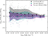Fig. 3. Comparison of the SFR(Hα) calibrations as a function of the intrinsic Hα luminosity: T19 calibration (gray) and the new SFR(Hα) calibrations given in Eq. (2) (cyan) and Eq. (3) (magenta). The vertical axis represents the SFR bias factor (ΔSFR ≡ SFR(Hα)/SFR10; closer to logΔSFR = 0 is better). The diamonds show the running median, with the error bars indicating the standard error on the median. The shaded regions indicate the 68% (1σ) confidence interval.

The SFR(Hα) calibration given in Eq. (2) corrects the SFRs by a factor that depends on L_Hα alone, which means that σ_SFR is neglected even for the updated calibration. To further improve on this, we added a correction to Eq. (2) that depended on the Hα equivalent width (EW_Hα). This choice was motivated by the fact that EW_Hα traces stellar metallicity and age, which both drive σ_SFR (Fig. 2). In addition, EW_Hα is only weakly sensitive to dust attenuation, which implies that dust corrections affect the results less than when other observables are used (e.g., M_UV). We therefore ran an OLS model that included EW_Hα, using the same training sample as in Eq. (2). The resulting SFR(Hα) calibration can be written as follows:

$$\begin{array}{cc}\hfill {log}_{10}\left[\frac{\mathrm{SFR}}{M_{\odot }{\mathrm{yr}}^{-1}}\right]& ={log}_{10}\left[\frac{L_{\mathrm{H}\alpha }^{\mathrm{int}}}{\mathrm{erg}{\mathrm{s}}^{-1}}\right]-41.45\hfill \\ \hfill & -0.01({log}_{10}\left[\frac{L_{\mathrm{H}\alpha }^{\mathrm{int}}}{\mathrm{erg}{\mathrm{s}}^{-1}}\right]-41.90)\hfill \\ \hfill & -0.26({log}_{10}\left[\frac{{\mathrm{EW}}_{\mathrm{H}\alpha }^{\mathrm{int}}}{\mathrm{\AA }}\right]-2.67),\hfill \end{array}$$(3)

where the last two terms are the effective corrections to Eq. (1). The new calibration yields RMSE = 0.11 dex on the training and test datasets, which is ≈0.02 dex lower than the RMSE calculated using Eq. (2), or ≈0.06 dex lower than the RMSE calculated using the T19 calibration (Z_* = Z_⊙). Figure 3 compares these calibrations as a function of $L_{\mathrm{H}\alpha }^{\mathrm{int}}$. In particular, this plot shows that the median Δ_SFR in the $L_{\mathrm{H}\alpha }^{\mathrm{int}}$ bins is within ±0.05 dex across the entire range of luminosities ($41.25<{log}_{10}(L_{\mathrm{H}\alpha }^{\mathrm{int}}/\mathrm{erg}{\mathrm{s}}^{-1})<43.25$) when using Eq. (2) or Eq. (3). This is an improvement over the T19 calibration, which overpredicted the SFRs by Δ_SFR ≳ 0.1 dex in galaxies with low to medium luminosities ($41.25<{log}_{10}(L_{\mathrm{H}\alpha }^{\mathrm{int}}/\mathrm{erg}{\mathrm{s}}^{-1})\lesssim 42.5$). The standard deviation of Δ_SFR in the $L_{\mathrm{H}\alpha }^{\mathrm{int}}$ bins (hereafter σ_ΔSFR) is nearly identical between the T19 calibration and the SFR(Hα) calibration given in Eq. (2) (σ_ΔSFR ≈ 0.11 dex), but it decreases by ≈0.03 dex (σ_ΔSFR ≈ 0.08 dex) for Eq. (3), especially at medium luminosities ($41.8\lesssim {log}_{10}(L_{\mathrm{H}\alpha }^{\mathrm{int}}/\mathrm{erg}{\mathrm{s}}^{-1})\lesssim 42.5$).

We also ran a similar model in which we replaced EW_Hα with [O III]/Hβ, which is a proxy for the gas-phase (and, to a weaker extent, stellar) metallicity. The resulting calibration showed the same performance as Eq. (3) (RMSE = 0.11 dex). Given the broader wavelength coverage required to measure [O III]/Hβ compared to EW_Hα, we found Eq. (3) to be more practical when applied to observations and hence used it as our best-performance calibration for the remainder of this paper.

4. Discussion

4.1. Implications

The Hα line has long been known as a reliable indicator of the SFR as it traces the ionizing photon luminosity from massive (M > 10 M_⊙) short-lived (t ≲ 10 Myr) stars (e.g., Kennicutt 1998). Over the past decades, Hα has been widely employed in numerous spectroscopic (e.g., Shim et al. 2009; Gunawardhana et al. 2013; Nagaraj et al. 2023) and narrow-band imaging (e.g., Ly et al. 2007; Hayes et al. 2010; Sobral et al. 2013) surveys to measure the cosmic SFH up to z ∼ 3. With the recent advent of sensitive near-IR spectroscopy at λ ∼ 3–5 μm, these measurements have been extended to z ≈ 3–6, in particular thanks to the JWST/NIRCam slitless spectroscopic observations of large samples of Hα-emitters at the same redshifts (e.g., Covelo-Paz et al. 2025; Fu et al. 2025; Lin et al. 2026).

As Hα observations become more accessible at high redshift, it is crucial to revisit the classical SFR(Hα) calibrations (e.g., Kennicutt 1998) that are commonly used at z ≲ 3. Based on a realistic galaxy simulation, we have shown that these calibrations bias the predicted SFRs under the physical conditions that are characteristic of high-redshift galaxies observed with JWST (i.e., a low metallicity and bursty star formation), potentially also affecting population statistics. To quantify this effect, we studied the effect of the metallicity- and age-dependent SFR bias (see Fig. 2) on the ρ_SFR measurements. Specifically, we converted the dust-corrected Hα luminosity function at z ∼ 6.3 presented in Schechter form by Fu et al. (2025) into the SFR function (SFRF). We performed this conversion by expressing the Hα luminosity via SFR using two SFR–L_Hα calibrations: the T19 calibration (Z_* = Z_⊙), and our new SFR(Hα) calibration given in Eq. (2), which, by design, takes the dependence of the SFR–L_Hα relation on metallicity into account. Following previous studies, we then integrated both SFRFs down to SFR = 0.24 M_⊙ yr⁻¹, which corresponds to M_UV = −17 (Bouwens et al. 2015). The resulting ρ_SFR decreased from ≈0.017 M_⊙ yr⁻¹ Mpc⁻³ to ≈0.015 M_⊙ yr⁻¹ Mpc⁻³, or by ≈12%, when using the new calibration. This suggests that the effect of the evolving SFR–L_Hα relation on ρ_SFR is moderate, likely because galaxies in which the SFR bias is highest contribute little to ρ_SFR. For example, galaxies with SFR < 10 M_⊙ yr⁻¹ contribute less than 30% to the total ρ_SFR. If we integrated the SFRF only up to SFR = 10 M_⊙ yr⁻¹, the change in ρ_SFR would be more pronounced: ρ_SFR would decrease by ≈29%.

The SFR bias also affects the correlations between the SFR and other galaxy properties, such as stellar mass. In Fig. 4, we show the SFR–M_* relation, also known as the star formation main sequence (SFMS; Noeske et al. 2007), in the JWST All the Little Things (ALT) survey (Naidu et al. 2024; Di Cesare et al. 2026). We applied different SFR(Hα) calibrations to the dust-corrected Hα luminosities and calculated the slope of the SFMS. The slope increased by Δ∂logSFR/∂logM_★ = 0.08 ± 0.02 (20 ± 6%) when we used Eq. (3) instead of the T19 calibration to calculate the SFRs. Equation (2) yields similar results, although they are less significant (Δ∂logSFR/∂logM_★ = 0.02 ± 0.03). In addition, the scatter in the SFMS decreases by Δσ_SFR ≈ 0.04 dex (≈14%) when using Eq. (3), most noticeably at the low-mass end (Δσ_SFR ≈ 0.06 dex at log₁₀(M_★/M_⊙) < 7). In contrast, Eq. (2) produces almost the same scatter as the T19 calibration (Δσ_SFR ≲ 0.01 dex). We note that the SFMS in Fig. 4 is affected by selection effects: some low-mass galaxies are not detected in observations due to their faintness, resulting in a shallow SFMS slope. Temporary cessation or strong suppression of star formation in galaxies during so-called mini-quenching events (e.g., Gelli et al. 2023; Looser et al. 2025) can further amplify this bias. However, a comprehensive discussion of caveats associated with the SFMS slope measurements is beyond the scope of this paper (this discussion can be found in Di Cesare et al. 2026).

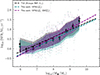Fig. 4. Star formation main sequence (SFMS) in the JWST ALT survey (Naidu et al. 2024; Di Cesare et al. 2026) with SFRs calculated using the T19 calibration (gray) and the new SFR(Hα) calibrations given in Eq. (2) (cyan) and Eq. (3) (magenta). The diamonds show the running median, with the error bars indicating the standard error on the median. The shaded regions indicate the 68% (1σ) confidence interval. The dashed lines show the linear regression fits to the SFMS individually for each calibration.

4.2. Dust attenuation

In Sect. 3, we ignored the effects of dust attenuation, assuming that the Hα line measurements (i.e., L_Hα and EW_Hα) can be corrected for these effects without errors. This assumption is also usually made for the SFR(Hα) calibrations presented in the literature. However, dust attenuation is known to be an important source of systematic error in the Hα-derived SFRs (e.g., Hopkins et al. 2001). This effect likely persists even at z ≳ 4 as the number of dust in Hα-emitters at these redshifts is found to be non-negligible (e.g., Covelo-Paz et al. 2025 reported the median A_Hα ≈ 0.5 mag for a sample of ≈1000 Hα-emitters at 4 ≲ z ≲ 6).

We tested the possibility of deriving SFRs directly from the observed Hα emission without prior dust corrections. We used the dust-attenuated Hα luminosity ($L_{\mathrm{H}\alpha }^{\mathrm{obs}}$) and equivalent width (${\mathrm{EW}}_{\mathrm{H}\alpha }^{\mathrm{obs}}$) from SPHINX, calculated as described in Sect. 2, and fit the same linear relations between the SFR, L_Hα, and EW_Hα as in Sect. 3. We present the resulting SFR(Hα) calibrations in Appendix B. The calibration that only depends on $L_{\mathrm{H}\alpha }^{\mathrm{obs}}$ (Eq. (B.1); Fig. 5, cyan) yields RMSE = 0.39 dex, while the calibration that additionally depends on ${\mathrm{EW}}_{\mathrm{H}\alpha }^{\mathrm{obs}}$ (Eq. (B.2); Fig. 5, magenta) yields RMSE = 0.22 dex. In both cases, the RMSE is significantly higher than the RMSEs calculated using the calibrations that are based on the intrinsic Hα properties (see Sect. 3). Moreover, the SFRs are significantly underestimated at high luminosities (${log}_{10}(L_{\mathrm{H}\alpha }^{\mathrm{int}}/\mathrm{erg}{\mathrm{s}}^{-1})\gtrsim 42.5$), with Eq. (B.1) and Eq. (B.2) producing the median Δ_SFR = −0.52 and Δ_SFR = −0.27, respectively. This can be explained by the fact that high-$L_{\mathrm{H}\alpha }^{\mathrm{int}}$ galaxies in SPHINX have very high attenuation values (A_Hα ≳ 2) on average, which we are unable to fully correct for while simultaneously trying to model the SFRs of low-$L_{\mathrm{H}\alpha }^{\mathrm{int}}$ galaxies. However, we caution that A_Hα like this are not reported in high-redshift observations (see Sect. 2), and it might therefore still be possible in practice to make accurate SFR estimates based on the dust-attenuated Hα.

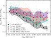Fig. 5. Same as Fig. 3, but for the observed (i.e., dust-attenuated) Hα. In addition to LHα and EWHα, two SFR(Hα) calibrations use the Balmer decrement (Hα/Hβ) to predict the SFR (orange and light blue). The equations for the new calibrations are given in Appendix B.

We also tested whether the Balmer decrement ($L_{\mathrm{H}\alpha }^{\mathrm{obs}}/L_{\mathrm{H}\beta }^{\mathrm{obs}}$; hereafter Hα/Hβ), whose measurements are commonly used to calculate the dust corrections for Hα, can be a useful parameter to include in the SFR(Hα) calibration. Interestingly, the Hα/Hβ-based calibration (Eq. (B.3); Fig. 5, orange) yielded RMSE = 0.29 dex, which is ≈0.07 dex higher than the RMSE calculated using the ${\mathrm{EW}}_{\mathrm{H}\alpha }^{\mathrm{obs}}$-based calibration. This indicates that Hα/Hβ is not as powerful as ${\mathrm{EW}}_{\mathrm{H}\alpha }^{\mathrm{obs}}$ in constraining the SFRs of the SPHINX galaxies. This result is surprising because Hα/Hβ is commonly regarded as a robust indicator of dust attenuation (A_Hα), while ${\mathrm{EW}}_{\mathrm{H}\alpha }^{\mathrm{obs}}$ is in principle mostly independent of it. However, we still find a negative correlation between ${\mathrm{EW}}_{\mathrm{H}\alpha }^{\mathrm{obs}}$ and A_Hα in SPHINX (r = −0.71, p < 10⁻⁶; Fig. 6), possibly because the amount of dust increases with the age of the stellar population, a parameter to which ${\mathrm{EW}}_{\mathrm{H}\alpha }^{\mathrm{obs}}$ is sensitive. Further, unlike Hα/Hβ, ${\mathrm{EW}}_{\mathrm{H}\alpha }^{\mathrm{obs}}$ correlates with stellar metallicity, allowing for an even more accurate prediction of the SFRs.

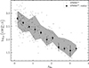Fig. 6. Hα equivalent width vs. dust attenuation in SPHINX. The diamonds show the running median, with the error bars indicating the standard error on the median. The shaded region indicates the 68% (1σ) confidence interval. We note that the AHα values from SPHINX might be overestimated compared to the typical AHα values measured in star-forming galaxies at z ≳ 3 (see Sect. 2).

Inclusion of both Hα/Hβ and ${\mathrm{EW}}_{\mathrm{H}\alpha }^{\mathrm{obs}}$ in the calibration (Eq. (B.4); see also Fig. 5, light blue) provides the best performance among the considered models (RMSE = 0.16 dex). Observationally, however, the Hα/Hβ measurements are hampered by slit losses and the requirement of a broader wavelength coverage. This implies that the benefits of including Hα/Hβ in the SFR(Hα) calibration are likely limited, with ${\mathrm{EW}}_{\mathrm{H}\alpha }^{\mathrm{obs}}$ remaining a key addition to the calibration.

4.3. Caveats

When using the SFR(Hα) calibrations given in Eq. (2) and Eq. (3), it is important to take proper account of the scope of applicability of these calibrations and the assumptions made to derive them. In particular, the selection criteria described in Sect. 2 imply that the new calibrations can be applied to a flux-limited sample when the following conditions are met:

• 4 ≲ z ≲ 10;

• $L_{\text{H}\alpha }^{\text{obs}}\gtrsim {10}^{41}$ erg s⁻¹.

It is already possible to extend the calibrations to $L_{\mathrm{H}\alpha }^{\mathrm{obs}}<{10}^{41}$ erg s⁻¹ with SPHINX, but a larger halo catalog than the currently available SPDRv1 catalog is needed to create a complete Hα sample down to very low luminosities. At low redshifts (z ≲ 4), the SFHs become less bursty and the metallicities increase, rendering the classical calibrations more suitable. Finally, at high redshift (z ≳ 10), it remains to be established whether the new calibrations can be used, as the physical conditions of star formation at these redshifts are poorly understood.

We also stress the fact that the new calibrations assumed the BPASS V2.2 SPS model with a Kroupa-type IMF (see Sect. 2). Figure 1 shows that the choice of the IMF significantly affects the predicted SFRs, resulting in a systematic error of up to ≈0.2 dex (see also Jeřábková et al. 2018, who studied the effect of a nonuniversal IMF on the SFR–L_Hα relation). The choice of the SPS model, in particular, whether the model includes binary stars, results in a smaller error (≈0.05 dex), possibly because binary stars have little effect on the LyC luminosity in the first ∼3 Myr of a stellar population when the bulk of ionizing photons is produced (e.g., Rosdahl et al. 2018), but this effect is still non-negligible. In the future, these systematic errors can be reduced by testing the SPS models and constraining the IMF at z > 4, for instance, by means of deep rest-frame UV spectroscopy (e.g., Steidel et al. 2016; Chisholm et al. 2019).

5. Summary

We studied the relation between Hα emission and the SFR in the SPHINX cosmological simulations at 4.64 ≤ z ≤ 10. Using the simulated galaxy data from the SPHINX Public Data Release, Version 1 (Katz et al. 2023), we selected a sample of star-forming galaxies that are representative of the Hα-emitter population routinely observed with JWST at z > 3. The median SFR–L_Hα relation in SPHINX exhibits a downturn at low luminosities (Fig. 1; ${log}_{10}(L_{\mathrm{H}\alpha }^{\mathrm{int}}/\mathrm{erg}{\mathrm{s}}^{-1})\sim 42.0$–42.5). This downturn is consistent with fainter galaxies having lower stellar metallicities (Z_★ ∼ 0.1 Z_⊙) and thus being more efficient producers of ionizing photons than brighter, relatively metal-enriched (Z_★ ≳ 0.3 Z_⊙) galaxies. Furthermore, the SFR–L_Hα relation exhibits a significant scatter at fixed luminosity, ranging from σ_SFR ≈ 0.04 dex at ${log}_{10}(L_{\mathrm{H}\alpha }^{\mathrm{int}}/\mathrm{erg}{\mathrm{s}}^{-1})=42.8$ to σ_SFR ≈ 0.17 dex at ${log}_{10}(L_{\mathrm{H}\alpha }^{\mathrm{int}}/\mathrm{erg}{\mathrm{s}}^{-1})=41.3$ (i.e., the scatter is larger at lower luminosities). We demonstrated that this scatter is primarily driven by the variations in the stellar metallicities and ages (Fig. 2), whereas other properties (e.g., M_★ and f_esc) play a less significant role.

Because of the metallicity dependence of the SFR–L_Hα relation, the classical SFR(Hα) calibrations (e.g., Kennicutt 1998; Eq. (1)) overestimate the SFRs of faint galaxies in SPHINX on average by Δ_SFR ≡ SFR(Hα)/SFR₁₀ ≳ 0.1 dex (Fig. 3, black). In Eq. (2), we proposed a new SFR(Hα) calibration that depends on the intrinsic Hα luminosity alone and reduces the error in the predicted SFRs by ΔRMSE ≈ 0.04 dex (Fig. 3, cyan). To address the scatter in the SFR–L_Hα relation, we proposed another SFR(Hα) calibration in Eq. (3) This calibration additionally depends on the Hα equivalent width, a parameter that is sensitive to the stellar metallicity and age (Fig. 2), and it further improved the SFR estimate, reducing the error by a total of ΔRMSE ≈ 0.06 dex (Fig. 3, magenta). The new SFR(Hα) calibrations affect the galaxy population statistics at high redshift (z ∼ 6): the inferred ρ_SFR decreases by ≈12%, and the slope of the SFMS increases by Δ∂logSFR/∂logM_★ = 0.08 ± 0.02 (Fig. 4).

Acknowledgments

We thank the anonymous referee for the insightful comments that helped improve the manuscript. We also thank Thibault Garel, Pascal Oesch, Irene Shivaei, Charlotte Simmonds, Andrew Hopkins, Daniel Schaerer, and Rashmi Gottumukkala for useful comments and productive discussions. We gratefully acknowledge support from the CBPsmn (PSMN, Pôle Scientifique de Modélisation Numérique) of the ENS de Lyon for the computing resources. Funded by the European Union (ERC, AGENTS, 101076224). Views and opinions expressed are however those of the author(s) only and do not necessarily reflect those of the European Union or the European Research Council. Neither the European Union nor the granting authority can be held responsible for them. This work made extensive use of several open-source software packages, and we gratefully acknowledge the efforts of their authors: NUMPY (Harris et al. 2020), ASTROPY (Astropy Collaboration 2022), MATPLOTLIB (Hunter 2007), IPYTHON (Perez & Granger 2007), and SCIKIT-LEARN (Pedregosa et al. 2011).

References

Appendix A: Timescales of star formation traced by Hα

It is commonly assumed in the literature that Hα traces star formation over the last t_SFR = 10 Myr. To test this, we use the SFHs published as part of SPDRv1 and calculate the average of the SFR over the last t_SFR = 1, 2, …, 30 Myr. We then calculate the correlation coefficients between $L_{\mathrm{H}\alpha }^{\mathrm{int}}$ and the SFRs averaged over different timescales. We find that Pearson’s r is highest between 4 Myr ≲ t ≲ 12 Myr (r > 0.95), with a maximum at t_SFR = 6 Myr (r = 0.98; Fig. A.1, dashed line). Similarly, Kendall’s τ peaks at t_SFR = 5 Myr (τ = 0.84; Fig. A.1, solid line). This suggests that a slightly shorter timescale (t_SFR = 5–6 Myr) might be more appropriate for Hα. Nevertheless, for consistency with previous works, we use the SFRs averaged over t_SFR = 10 Myr throughout this paper.

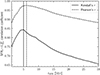Fig. A.1. Correlation coefficients between the SFR and $L_{\mathrm{H}\alpha }^{\mathrm{int}}$ as a function of the star formation timescale, tSFR.

Appendix B: SFR(Hα) calibrations for the dust-attenuated Hα line measurements

$$\begin{array}{c}\hfill \begin{array}{cc}\hfill {log}_{10}\left[\frac{\mathrm{SFR}}{M_{\odot }{\mathrm{yr}}^{-1}}\right]=& {log}_{10}\left[\frac{L_{\mathrm{H}\alpha }^{\mathrm{obs}}}{\mathrm{erg}{\mathrm{s}}^{-1}}\right]-41.00\hfill \\ \hfill & +0.66({log}_{10}\left[\frac{L_{\mathrm{H}\alpha }^{\mathrm{obs}}}{\mathrm{erg}{\mathrm{s}}^{-1}}\right]-41.46)\hfill \end{array}\end{array}$$(B.1)

$$\begin{array}{c}\hfill \begin{array}{cc}\hfill {log}_{10}\left[\frac{\mathrm{SFR}}{M_{\odot }{\mathrm{yr}}^{-1}}\right]=& {log}_{10}\left[\frac{L_{\mathrm{H}\alpha }^{\mathrm{obs}}}{\mathrm{erg}{\mathrm{s}}^{-1}}\right]-41.00\hfill \\ \hfill & +0.23({log}_{10}\left[\frac{L_{\mathrm{H}\alpha }^{\mathrm{obs}}}{\mathrm{erg}{\mathrm{s}}^{-1}}\right]-41.46)\hfill \\ \hfill & -0.67({log}_{10}\left[\frac{{\mathrm{EW}}_{\mathrm{H}\alpha }^{\mathrm{obs}}}{\mathrm{\AA }}\right]-2.41)\hfill \end{array}\end{array}$$(B.2)

$$\begin{array}{c}\hfill \begin{array}{cc}\hfill {log}_{10}\left[\frac{\mathrm{SFR}}{M_{\odot }{\mathrm{yr}}^{-1}}\right]=& {log}_{10}\left[\frac{L_{\mathrm{H}\alpha }^{\mathrm{obs}}}{\mathrm{erg}{\mathrm{s}}^{-1}}\right]-41.00\hfill \\ \hfill & +0.58({log}_{10}\left[\frac{L_{\mathrm{H}\alpha }^{\mathrm{obs}}}{\mathrm{erg}{\mathrm{s}}^{-1}}\right]-41.46)\hfill \\ \hfill & +5.81({log}_{10}(L_{\mathrm{H}\alpha }^{\mathrm{obs}}/L_{\mathrm{H}\alpha }^{\mathrm{obs}})-0.51)\hfill \end{array}\end{array}$$(B.3)

$$\begin{array}{c}\hfill \begin{array}{cc}\hfill {log}_{10}\left[\frac{\mathrm{SFR}}{M_{\odot }{\mathrm{yr}}^{-1}}\right]=& {log}_{10}\left[\frac{L_{\mathrm{H}\alpha }^{\mathrm{obs}}}{\mathrm{erg}{\mathrm{s}}^{-1}}\right]-41.00\hfill \\ \hfill & +0.22({log}_{10}\left[\frac{L_{\mathrm{H}\alpha }^{\mathrm{obs}}}{\mathrm{erg}{\mathrm{s}}^{-1}}\right]-41.46)\hfill \\ \hfill & -0.59({log}_{10}\left[\frac{{\mathrm{EW}}_{\mathrm{H}\alpha }^{\mathrm{obs}}}{\mathrm{\AA }}\right]-2.41)\hfill \\ \hfill & +3.74({log}_{10}(L_{\mathrm{H}\alpha }^{\mathrm{obs}}/L_{\mathrm{H}\beta }^{\mathrm{obs}})-0.51)\hfill \end{array}\end{array}$$(B.4)

All Figures

Fig. 1. Intrinsic SFR–LHα relation in the SPHINX20 cosmological simulation, color-coded by the stellar metallicity. The SFR values are averaged over t = 10 Myr, i.e., the typical lifetime of stars traced by Hα. The diamonds show the median SFR in the bins of $L_{\mathrm{H}\alpha }^{\mathrm{int}}$, with the error bars showing the standard error on the median. The shaded region indicates the 68% (1σ) confidence interval. The diagonal lines show the SFR(Hα) calibrations from the literature, i.e. (top to bottom), the original K98 calibration, the K98 calibration converted into the Kroupa IMF, and two calibrations from T19 calculated for the Kroupa IMF and two different metallicities (Z* = Z⊙ and Z* = 0.1 Z⊙, respectively).

In the text

	Fig. 2. SFR bias factor (ΔSFR ≡ SFR(Hα)/SFR10) as a function of stellar metallicity (top) and age (bottom) in SPHINX, color-coded by EWHα. The SFR(Hα) values are calculated using the T19 calibration (Z* = Z⊙). The diamonds show the running median, with the error bars indicating the standard error on the median. The shaded region indicates the 68% (1σ) confidence interval.
In the text

Fig. 3. Comparison of the SFR(Hα) calibrations as a function of the intrinsic Hα luminosity: T19 calibration (gray) and the new SFR(Hα) calibrations given in Eq. (2) (cyan) and Eq. (3) (magenta). The vertical axis represents the SFR bias factor (ΔSFR ≡ SFR(Hα)/SFR10; closer to logΔSFR = 0 is better). The diamonds show the running median, with the error bars indicating the standard error on the median. The shaded regions indicate the 68% (1σ) confidence interval.

In the text

Fig. 4. Star formation main sequence (SFMS) in the JWST ALT survey (Naidu et al. 2024; Di Cesare et al. 2026) with SFRs calculated using the T19 calibration (gray) and the new SFR(Hα) calibrations given in Eq. (2) (cyan) and Eq. (3) (magenta). The diamonds show the running median, with the error bars indicating the standard error on the median. The shaded regions indicate the 68% (1σ) confidence interval. The dashed lines show the linear regression fits to the SFMS individually for each calibration.

In the text

	Fig. 5. Same as Fig. 3, but for the observed (i.e., dust-attenuated) Hα. In addition to LHα and EWHα, two SFR(Hα) calibrations use the Balmer decrement (Hα/Hβ) to predict the SFR (orange and light blue). The equations for the new calibrations are given in Appendix B.
In the text

	Fig. 6. Hα equivalent width vs. dust attenuation in SPHINX. The diamonds show the running median, with the error bars indicating the standard error on the median. The shaded region indicates the 68% (1σ) confidence interval. We note that the AHα values from SPHINX might be overestimated compared to the typical AHα values measured in star-forming galaxies at z ≳ 3 (see Sect. 2).
In the text

	Fig. A.1. Correlation coefficients between the SFR and $L_{\mathrm{H}\alpha }^{\mathrm{int}}$ as a function of the star formation timescale, tSFR.
In the text

References

- Asada, Y., Sawicki, M., Abraham, R., et al. 2024, MNRAS, 527, 11372 [Google Scholar]
- Astropy Collaboration (Price-Whelan, A. M., et al.) 2022, ApJ, 935, 167 [NASA ADS] [CrossRef] [Google Scholar]
- Behroozi, P., Wechsler, R. H., Hearin, A. P., & Conroy, C. 2019, MNRAS, 488, 3143 [NASA ADS] [CrossRef] [Google Scholar]
- Bezanson, R., Labbe, I., Whitaker, K. E., et al. 2024, ApJ, 974, 92 [NASA ADS] [CrossRef] [Google Scholar]
- Bouché, N., Dekel, A., Genzel, R., et al. 2010, ApJ, 718, 1001 [Google Scholar]
- Bouwens, R. J., Illingworth, G. D., Oesch, P. A., et al. 2015, ApJ, 803, 34 [Google Scholar]
- Carvajal-Bohorquez, C., Ciesla, L., Laporte, N., et al. 2025, A&A, 704, A290 [NASA ADS] [CrossRef] [EDP Sciences] [Google Scholar]
- Chisholm, J., Rigby, J. R., Bayliss, M., et al. 2019, ApJ, 882, 182 [Google Scholar]
- Chruślińska, M., Pakmor, R., Matthee, J., & Matsuno, T. 2024, A&A, 686, A186 [NASA ADS] [CrossRef] [EDP Sciences] [Google Scholar]
- Clarke, L., Shapley, A. E., Sanders, R. L., et al. 2024, ApJ, 977, 133 [NASA ADS] [CrossRef] [Google Scholar]
- Cole, J. W., Papovich, C., Finkelstein, S. L., et al. 2025, ApJ, 979, 193 [Google Scholar]
- Covelo-Paz, A., Giovinazzo, E., Oesch, P. A., et al. 2025, A&A, 694, A178 [NASA ADS] [CrossRef] [EDP Sciences] [Google Scholar]
- Cullen, F., McLure, R. J., Dunlop, J. S., et al. 2019, MNRAS, 487, 2038 [Google Scholar]
- Curti, M., Maiolino, R., Curtis-Lake, E., et al. 2024, A&A, 684, A75 [NASA ADS] [CrossRef] [EDP Sciences] [Google Scholar]
- Davies, L. J. M., Lagos, C. d. P., Katsianis, A., et al. 2019, MNRAS, 483, 1881 [Google Scholar]
- De Looze, I., Cormier, D., Lebouteiller, V., et al. 2014, A&A, 568, A62 [NASA ADS] [CrossRef] [EDP Sciences] [Google Scholar]
- Di Cesare, C., Matthee, J., Naidu, R. P., et al. 2026, A&A, 707, A129 [NASA ADS] [CrossRef] [EDP Sciences] [Google Scholar]
- Endsley, R., Stark, D. P., Whitler, L., et al. 2024, MNRAS, 533, 1111 [NASA ADS] [CrossRef] [Google Scholar]
- Ferland, G. J., Chatzikos, M., Guzmán, F., et al. 2017, Rev. Mex. Astron. Astrofis., 53, 385 [NASA ADS] [Google Scholar]
- Fisher, R., Bowler, R. A. A., Stefanon, M., et al. 2025, MNRAS, 539, 109 [Google Scholar]
- Flores Velázquez, J. A., Gurvich, A. B., Faucher-Giguère, C.-A., et al. 2021, MNRAS, 501, 4812 [CrossRef] [Google Scholar]
- Fu, S., Sun, F., Jiang, L., et al. 2025, ApJ, 987, 186 [Google Scholar]
- Gelli, V., Salvadori, S., Ferrara, A., Pallottini, A., & Carniani, S. 2023, ApJ, 954, L11 [NASA ADS] [CrossRef] [Google Scholar]
- Götberg, Y., de Mink, S. E., & Groh, J. H. 2017, A&A, 608, A11 [NASA ADS] [CrossRef] [EDP Sciences] [Google Scholar]
- Gunawardhana, M. L. P., Hopkins, A. M., Bland-Hawthorn, J., et al. 2013, MNRAS, 433, 2764 [NASA ADS] [CrossRef] [Google Scholar]
- Hao, C.-N., Kennicutt, R. C., Johnson, B. D., et al. 2011, ApJ, 741, 124 [Google Scholar]
- Harris, C. R., Millman, K. J., van der Walt, S. J., et al. 2020, Nature, 585, 357 [NASA ADS] [CrossRef] [Google Scholar]
- Hayes, M., Schaerer, D., & Östlin, G. 2010, A&A, 509, L5 [NASA ADS] [CrossRef] [EDP Sciences] [Google Scholar]
- Hopkins, A. M., Connolly, A. J., Haarsma, D. B., & Cram, L. E. 2001, AJ, 122, 288 [NASA ADS] [CrossRef] [Google Scholar]
- Hunter, J. D. 2007, Comput. Sci. Eng., 9, 90 [NASA ADS] [CrossRef] [Google Scholar]
- Iyer, K. G., Tacchella, S., Genel, S., et al. 2020, MNRAS, 498, 430 [NASA ADS] [CrossRef] [Google Scholar]
- Jeřábková, T., Zonoozi, A. H., Kroupa, P., et al. 2018, A&A, 620, A39 [NASA ADS] [CrossRef] [EDP Sciences] [Google Scholar]
- Katz, H., Rosdahl, J., Kimm, T., et al. 2023, Open J. Astrophys., 6, 44 [NASA ADS] [CrossRef] [Google Scholar]
- Kennicutt, R. C., Jr. 1998, ARA&A, 36, 189 [Google Scholar]
- Kennicutt, R. C., & Evans, N. J. 2012, ARA&A, 50, 531 [NASA ADS] [CrossRef] [Google Scholar]
- Kroupa, P. 2001, MNRAS, 322, 231 [NASA ADS] [CrossRef] [Google Scholar]
- Laursen, P., Sommer-Larsen, J., & Andersen, A. C. 2009, ApJ, 704, 1640 [Google Scholar]
- Leitherer, C., Schaerer, D., Goldader, J. D., et al. 1999, ApJS, 123, 3 [Google Scholar]
- Lilly, S. J., Carollo, C. M., Pipino, A., Renzini, A., & Peng, Y. 2013, ApJ, 772, 119 [NASA ADS] [CrossRef] [Google Scholar]
- Lin, X., Egami, E., Sun, F., et al. 2026, ApJ, 997, 207 [Google Scholar]
- Looser, T. J., D’Eugenio, F., Maiolino, R., et al. 2025, A&A, 697, A88 [NASA ADS] [CrossRef] [EDP Sciences] [Google Scholar]
- Ly, C., Malkan, M. A., Kashikawa, N., et al. 2007, ApJ, 657, 738 [NASA ADS] [CrossRef] [Google Scholar]
- Markov, V., Gallerani, S., Ferrara, A., et al. 2025, Nat. Astron., 9, 458 [Google Scholar]
- Mascia, S., Pentericci, L., Calabrò, A., et al. 2024, A&A, 685, A3 [NASA ADS] [CrossRef] [EDP Sciences] [Google Scholar]
- Matthee, J., & Schaye, J. 2019, MNRAS, 484, 915 [CrossRef] [Google Scholar]
- Matthee, J., Feltre, A., Maseda, M., et al. 2022, A&A, 660, A10 [NASA ADS] [CrossRef] [EDP Sciences] [Google Scholar]
- Meyer, R. A., Oesch, P. A., Giovinazzo, E., et al. 2024, MNRAS, 535, 1067 [CrossRef] [Google Scholar]
- Michel-Dansac, L., Blaizot, J., Garel, T., et al. 2020, A&A, 635, A154 [EDP Sciences] [Google Scholar]
- Nagaraj, G., Ciardullo, R., Bowman, W. P., Lawson, A., & Gronwall, C. 2023, ApJ, 943, 5 [Google Scholar]
- Naidu, R. P., Matthee, J., Kramarenko, I., et al. 2024, Open J. Astrophys., submitted [arXiv:2410.01874] [Google Scholar]
- Noeske, K. G., Weiner, B. J., Faber, S. M., et al. 2007, ApJ, 660, L43 [CrossRef] [Google Scholar]
- Pedregosa, F., Varoquaux, G., Gramfort, A., et al. 2011, J. Mach. Learn. Res., 12, 2825 [Google Scholar]
- Perez, F., & Granger, B. E. 2007, Comput. Sci. Eng., 9, 21 [Google Scholar]
- Pirie, C. A., Best, P. N., Duncan, K. J., et al. 2025, MNRAS, 541, 1348 [Google Scholar]
- Rosdahl, J., Blaizot, J., Aubert, D., Stranex, T., & Teyssier, R. 2013, MNRAS, 436, 2188 [Google Scholar]
- Rosdahl, J., Katz, H., Blaizot, J., et al. 2018, MNRAS, 479, 994 [NASA ADS] [Google Scholar]
- Rosdahl, J., Blaizot, J., Katz, H., et al. 2022, MNRAS, 515, 2386 [CrossRef] [Google Scholar]
- Salpeter, E. E. 1955, ApJ, 121, 161 [Google Scholar]
- Scholte, D., Cullen, F., Carnall, A. C., et al. 2025, MNRAS, 540, 1800 [Google Scholar]
- Shim, H., Colbert, J., Teplitz, H., et al. 2009, ApJ, 696, 785 [NASA ADS] [CrossRef] [Google Scholar]
- Shivaei, I., Naidu, R. P., Rodríguez Montero, F., et al. 2025, A&A, submitted [arXiv:2509.01795] [Google Scholar]
- Sobral, D., Smail, I., Best, P. N., et al. 2013, MNRAS, 428, 1128 [NASA ADS] [CrossRef] [Google Scholar]
- Sparre, M., Hayward, C. C., Springel, V., et al. 2015, MNRAS, 447, 3548 [Google Scholar]
- Stanway, E. R., & Eldridge, J. J. 2018, MNRAS, 479, 75 [NASA ADS] [CrossRef] [Google Scholar]
- Steidel, C. C., Strom, A. L., Pettini, M., et al. 2016, ApJ, 826, 159 [NASA ADS] [CrossRef] [Google Scholar]
- Sun, F., Wang, F., Yang, J., et al. 2025, ApJ, 980, 12 [Google Scholar]
- Tacchella, S., Forbes, J. C., & Caplar, N. 2020, MNRAS, 497, 698 [Google Scholar]
- Teyssier, R. 2002, A&A, 385, 337 [CrossRef] [EDP Sciences] [Google Scholar]
- Theios, R. L., Steidel, C. C., Strom, A. L., et al. 2019, ApJ, 871, 128 [NASA ADS] [CrossRef] [Google Scholar]
- Wan, J. T., Tacchella, S., D’Eugenio, F., Johnson, B. D., & van der Wel, A. 2025, MNRAS, 539, 2891 [Google Scholar]
- Wang, E., & Lilly, S. J. 2020, ApJ, 892, 87 [Google Scholar]
- Weibel, A., Oesch, P. A., Barrufet, L., et al. 2024, MNRAS, 533, 1808 [NASA ADS] [CrossRef] [Google Scholar]
- Wilkins, S. M., Lovell, C. C., & Stanway, E. R. 2019, MNRAS, 490, 5359 [NASA ADS] [CrossRef] [Google Scholar]
- Zavala, J. A., Casey, C. M., Manning, S. M., et al. 2021, ApJ, 909, 165 [CrossRef] [Google Scholar]
Throughout this work, we assume a negligible contribution of active galactic nuclei to the Hα emission.
Hereafter, stellar metallicities (and ages) of SPHINX galaxies are weighted by the LyC luminosity.