© The Authors 2026

1. Introduction

Space weather refers to variations in the space environment between the Sun and Earth. It is primarily concerned with the Sun’s influence on our Solar System due to changes in its magnetic activity and associated phenomena. Predicting space weather is vital because of its significant socio-economic impact on systems such as radio communications, satellite avionics, Global Positioning System (GPS) navigation, and electrical power grids on Earth. Space-weather variations also pose a potential health risk to astronauts and aeroplane passengers traveling on high-altitude aviation flights. Therefore, a deep understanding of the dynamics and structure of the solar atmosphere is necessary to model space-weather phenomena. Global magnetohydrodynamic (MHD) and multi-fluid coronal models of the solar atmosphere are critical for space-weather forecasting as they are the first link in the Sun-to-Earth model chains used for space-weather predictions (Poedts 2019; Poedts et al. 2020a,b). Such model chains have become indispensable tools for advancing our understanding of space weather, particularly because they can simulate the entire solar heliosphere and the propagation of coronal mass ejections (CMEs) and other associated solar phenomena (Feng 2019).

The solar atmosphere comprises four distinct layers, each with distinct physical properties: the photosphere, the chromosphere, the transition region, and the solar corona. The key space-weather phenomena originating from these regions include solar flares, CMEs, solar energetic particle (SEP) events, and high-speed solar-wind streams (HSS). These phenomena alter the ambient plasma, magnetic fields, radiation, and particle flow in space, as well as their interactions with planets’ magnetospheres (Gopalswamy 2022). The single-fluid MHD model provides valuable insights, facilitating advances in our understanding of the solar corona, the outermost layer of the solar atmosphere, with temperatures ranging from 1 − 3 MK. At such high temperatures, the plasma is anticipated to be nearly completely ionised, and therefore, the problem is usually approached using traditional single-fluid MHD models (Mikić et al. 1999; Usmanov & Goldstein 2003; Riley et al. 2001; Hu et al. 2008; Jin et al. 2016; Gombosi et al. 2018; Goedbloed et al. 2019; Downs et al. 2021; Iijima et al. 2023). Coronal MHD simulations have become an increasingly prevalent tool for modeling, primarily due to recent developments and the availability of high-performance computing. These enhancements have enabled two-dimensional (2-D) and three-dimensional (3-D) MHD simulations, allowing for more sophisticated and realistic modeling of coronal dynamics. The intricate complexity of a solar corona and its dynamic nature have attracted significant scientific attention over the past half a century (Schnack 1994; Aschwanden 2019; Aslanyan et al. 2024). Quantitative modeling and understanding the underlying complexity are among the significant challenges in heliophysics that remain to be overcome. Reviews such as Kuperus et al. (1981), Cargill (2000), Califano (2000), Einaudi & Velli (2005), Sakurai (2017), and Lu et al. (2024) cover many details related to the heating of the solar corona and its implications for space-weather forecasting.

The studies mentioned above have significantly advanced our understanding of coronal dynamics. These advancements are critical, particularly given the complexity of the corona, where even high-temperature plasma can harbour remnants of neutral particles, potentially leading to ionization, recombination, and charge exchange. (Sime & McCabe 1990; Fontenla et al. 1993; Dorotovic et al. 1997; Zaqarashvili et al. 2011; Vial & Chane-Yook 2016) Previous studies have shown that, despite their low concentration, neutrals can have a small but noticeable impact on the flow field (e.g., Andretta & Jones 1997, Braileanu et al. 2019, Khomenko et al. 2021). During solar maximum, when CMEs, flares, and prominence eruptions are most frequent, neutrals in the solar corona may amplify such effects. For example, Pagano et al. (2020) found that the CMEs’ leading edges can contain orders of magnitude more neutral-rich hydrogen than equilibrium predicts. Such neutrals affect the energy transport and diagnostics in solar eruptions. The neutral fractions in the solar atmosphere may affect both large-scale activity and small-scale dynamics, thus altering the wave propagation and shock formation (Judge 2020; Melis et al. 2021). In similar lines, the studies by Tu & Marsch (1997) and Martínez-Gómez et al. (2022) account for the two-fluid effects in the solar corona. All these studies imply that even a tiny percentage of neutrals can locally influence the ion temperature and velocity via the momentum and energy source terms (Brchnelova et al. 2023) and challenge the traditional assumption that neutrals do not significantly impact the solar corona dynamics (Martínez-Sykora et al. 2015). Therefore, a more comprehensive approach, beyond single-fluid models involving multi-fluid MHD (MF-MHD hereafter), is necessary to fully capture the complexity of the partially ionized plasma in the solar corona. Considering MF-MHD effects, the plasma model is expected to offer a more comprehensive understanding of the solar atmosphere by accounting for momentum and energy exchange between the constituent species. This may enhance space-weather predictions and provide a more accurate description of the intricate physics of the partially ionized corona.

Modern plasma codes employ computational fluid-dynamics methods to obtain accurate results for numerous coronal features and to forecast space-weather events. A novel, data-driven 3-D global coronal model, COolfluid COronal uNstrUcTure (COCONUT), has been developed in this context (Perri et al. 2022, 2023). This model, built on the Computational Object-Oriented Libraries for Fluid Dynamics (COOLFluiD) numerical code (Lani et al. 2005), aims to replace traditional semi-empirical models, such as the Wang-Sheeley-Arge (WSA) model (Wang & Sheeley 1990), which are often used in operational space-weather forecasting contexts. In light of the above studies, to seek more sophisticated and realistic modeling of the coronal dynamics and mark the importance of the multi-fluid model, this paper aims to build upon the polytropic MF-MHD framework established in Brchnelova et al. (2023) by introducing new source and sink terms in the energy equations and upgrading it to a complete MF-MHD COCONUT model. This extension investigates two-fluid models to enhance our understanding of the impacts of two-fluid effects on global coronal modeling and space-weather forecasting. We refer to this approach as the thermodynamic MF-MHD model (TMF-MHD).

The COCONUT model has shown good accuracy and stability in strenuous cases representative of a solar maximum and minimum. Having passed a wide range of benchmark tests, the code has demonstrated its precision in handling simple cases of dipole and quadrupole configurations and diverse solar minimum and solar maximum magnetograms. Recent publications provide a thorough description of the COCONUT model (Perri et al. 2022, 2023). Modelling the solar atmosphere during solar maximum poses significant challenges due to steep gradients in various parameters, including intense magnetic fields and the rapid evolution of small-scale structures. Notably, Kuźma et al. (2023) reported a good correlation of simulation results produced by the COCONUT model during both the solar maximum and minimum for the first time. This includes accurate representations of solar streamer positions, orientations, and shapes, further validating the model in solar physics research.

The contents of this paper are organized as follows. Sect. 2 introduces the TMF-MHD model, which defines the dynamics of the solar atmosphere. Sect. 3 summarizes the source-sink terms used in the energy equations and describes the coronal-heating function. Sect. 4 provides a brief overview of the adopted numerical setup. Sect. 5 summarizes the key results of this paper. Sect. 6 elaborates on the influence of the source-sink terms on the magnetic topology. Sect. 7 discusses the performance of the model, followed by a conclusion and discussion in Sect. 8.

2. Multi-fluid, ion-neutral formulation

The model comprises a set of equations that govern the multi-fluid ion-neutral system and is solved by the COOLFluid code. Brchnelova et al. (2023) gives in-depth coverage of the equations described below.

2.1. Mass-continuity equations

The mass-continuity equations are as follows:

$$\begin{array}{cc}\hfill \frac{\partial n_{\mathrm{i}}}{\partial t}+\mathrm{\nabla }·(n_{\mathrm{i}}{\mathbf{V}}_{\mathrm{i}})& ={\mathrm{\Gamma }}_{\mathrm{i}}^{\mathrm{ion}}+{\mathrm{\Gamma }}_{\mathrm{i}}^{\mathrm{rec}},\hfill \end{array}$$(1)

$$\begin{array}{cc}\hfill \frac{\partial n_{\mathrm{n}}}{\partial t}+\mathrm{\nabla }·(n_{\mathrm{n}}{\mathbf{V}}_{\mathrm{n}})& ={\mathrm{\Gamma }}_{\mathrm{n}}^{\mathrm{rec}}+{\mathrm{\Gamma }}_{\mathrm{n}}^{\mathrm{ion}}.\hfill \end{array}$$(2)

Here, Γs denote the ionization and recombination rates given as

$$\begin{array}{c}\hfill {\mathrm{\Gamma }}_{\mathrm{n}}^{\mathrm{ion}}\equiv -n_{\mathrm{n}}{v}^{\mathrm{ion}},{\mathrm{\Gamma }}_{\mathrm{i}}^{\mathrm{rec}}\equiv -n_{\mathrm{i}}{v}^{\mathrm{rec}}.\end{array}$$(3)

Here, v^ion, rec is the ionization and recombination frequency defined as

$$\begin{array}{cc}\hfill v^{\mathrm{ion}}& =n_{\mathrm{e}}\left\{\frac{2.91\times {10}^{-14}}{0.232+{\varphi }_{\mathrm{ion}}/T_{\mathrm{e}}^{\ast }}\right\}{\left(\frac{{\varphi }_{\mathrm{ion}}}{T_{\mathrm{e}}^{\ast }}\right)}^{0.39}{e}^{\frac{-{\varphi }_{\mathrm{ion}}}{T_{\mathrm{e}}^{\ast }}}{\mathrm{m}}^3{\mathrm{s}}^{-1},\hfill \end{array}$$(4)

$$\begin{array}{cc}\hfill v^{\mathrm{rec}}& =2.6\times {10}^{-19}\frac{n_{\mathrm{e}}}{\sqrt{T_{\mathrm{e}}^{\ast }}}{\mathrm{m}}^3{\mathrm{s}}^{-1}.\hfill \end{array}$$(5)

In these equations, v^ion is adopted from the analytic fit of Voronov (1997), while v^rec, according to Nahar (2021), with ϕ_ion, is the ionization potential of the H-atom set equal to 13.6 eV (Meier & Shumlak 2012). These ionization and recombination rates are valid only for hydrogen.

2.2. Momentum equations

The momentum equations are as follows:

$$\begin{array}{cc}& \frac{\partial }{\partial t}(m_{\mathrm{i}}{n}_{\mathrm{i}}{\mathbf{V}}_{\mathrm{i}})+\mathrm{\nabla }·(m_{\mathrm{i}}{n}_{\mathrm{i}}{\mathbf{V}}_{\mathrm{i}}{\mathbf{V}}_{\mathrm{i}}+{\mathbb{P}}_{\mathrm{i}})=q_{\mathrm{i}}{n}_{\mathrm{i}}(\mathbf{E}+{\mathbf{V}}_{\mathrm{i}}\times \mathbf{B})\hfill \\ \hfill & +{\mathbf{R}}_{\mathrm{i}}^{\mathrm{in}}+{\mathbf{S}}_{\mathrm{i}}^{\mathrm{ion}}+{\mathbf{S}}_{\mathrm{i}}^{\mathrm{ex}}+m_{\mathrm{i}}{n}_{\mathrm{i}}\mathbf{g},\hfill \end{array}$$(6)

$$\begin{array}{cc}& \frac{\partial }{\partial t}(m_{\mathrm{n}}{n}_{\mathrm{n}}{\mathbf{V}}_{\mathrm{n}})+\mathrm{\nabla }·(m_{\mathrm{n}}{n}_{\mathrm{n}}{\mathbf{V}}_{\mathrm{n}}{\mathbf{V}}_{\mathrm{n}}+{\mathbb{P}}_{\mathrm{n}})=-{\mathbf{R}}_{\mathrm{n}}^{\mathrm{in}}+{\mathbf{S}}_{\mathrm{n}}^{\mathrm{ion}}\hfill \\ \hfill & +{\mathbf{S}}_{\mathrm{n}}^{\mathrm{ex}}+m_{\mathrm{n}}{n}_{\mathrm{n}}\mathbf{g}.\hfill \end{array}$$(7)

The terms describing momentum due to ionization, ${\mathbf{S}}_{\mathrm{i},\mathrm{n}}^{\mathrm{ion}}$, and charge exchange, ${\mathbf{S}}_{\mathrm{i},\mathrm{n}}^{\mathrm{ex}}$, are given as

$$\begin{array}{cc}\hfill {\mathbf{S}}_{\mathrm{i}}^{\mathrm{ion}}& =-{\mathbf{S}}_{\mathrm{n}}^{\mathrm{ion}}={\mathrm{\Gamma }}_{\mathrm{i}}^{\mathrm{ion}}{m}_{\mathrm{n}}{\mathbf{V}}_{\mathrm{n}}-{\mathrm{\Gamma }}_{\mathrm{n}}^{\mathrm{rec}}{m}_{\mathrm{i}}{\mathbf{V}}_{\mathrm{i}},\hfill \end{array}$$(8)

$$\begin{array}{cc}\hfill {\mathbf{S}}_{\mathrm{i}}^{\mathrm{ex}}& =-{\mathbf{S}}_{\mathrm{n}}^{\mathrm{ex}}={\mathrm{\Gamma }}^{\mathrm{ex}}{m}_{\mathrm{i}}({\mathbf{V}}_{\mathrm{n}}-{\mathbf{V}}_{\mathrm{i}})+{\mathbf{R}}_{\mathrm{in}}^{\mathrm{ex}}-{\mathbf{R}}_{\mathrm{ni}}^{\mathrm{ex}}.\hfill \end{array}$$(9)

Here, Γ^ex is the charge-exchange collision rate. The momentum collision terms, ${\mathbf{R}}_{\mathrm{i}}^{\mathrm{in}},{\mathbf{R}}_{\mathrm{n}}^{\mathrm{ni}}$, are defined as

$$\begin{array}{c}\hfill {\mathbf{R}}_{\mathrm{i}}^{\mathrm{in}}=-{\mathbf{R}}_{\mathrm{n}}^{\mathrm{ni}}=m_{\mathrm{in}}{n}_{\mathrm{i}}{v}_{\mathrm{in}}({\mathbf{V}}_{\mathrm{n}}-{\mathbf{V}}_{\mathrm{i}}),\end{array}$$(10)

with the ion-neutral, ν_in, and neutral-ion, ν_ni, collision frequencies given by

$$\begin{array}{c}\hfill v_{\mathrm{in}}=n_{\mathrm{n}}{\mathrm{\Sigma }}_{\mathrm{in}}\sqrt{\frac{8k_B{T}_{\mathrm{in}}}{\pi m_{\mathrm{in}}}},v_{\mathrm{ni}}=n_{\mathrm{n}}{\mathrm{\Sigma }}_{\mathrm{ni}}\sqrt{\frac{8k_B{T}_{\mathrm{in}}}{\pi m_{\mathrm{ni}}}}·\end{array}$$(11)

Here, Σ_ni and Σ_in represent the collisional cross sections taken here equal to 1.41 × 10⁻¹⁹ m² (Wargnier et al. 2022), while T_in, T_ni and m_in, m_ni are, respectively, the average temperature and mass defined as

$$\begin{array}{c}\hfill T_{\mathrm{in}}=T_{\mathrm{ni}}=\frac{T_{\mathrm{i}}+T_{\mathrm{n}}}{2}\text{and}{m}_{\mathrm{in}}=m_{\mathrm{ni}}=\frac{m_{\mathrm{i}}{m}_{\mathrm{n}}}{m_{\mathrm{i}}+m_{\mathrm{n}}}·\end{array}$$(12)

The terms ${\mathbf{R}}_{\mathrm{in}}^{\mathrm{ex}}$ and ${\mathbf{R}}_{\mathrm{ni}}^{\mathrm{ex}}$ in Eq. (9) represent the momentum transfer caused by charge exchange, and they read as

$$\begin{array}{cc}\hfill {\mathbf{R}}_{\mathrm{in}}^{\mathrm{ex}}& =-\frac{m_{\mathrm{i}}{\sigma }_{\mathrm{ex}}{n}_{\mathrm{i}}{n}_{\mathrm{n}}{V}_{\mathrm{ex}}{\mathbf{V}}_{\mathrm{in}}{v}_{{\mathrm{T}}_{}}^2}{\sqrt{(\frac{16}{\pi }{v}_{{\mathrm{T}}_{\mathrm{i}}}^2+4v_{\mathrm{in}}^2)+\frac{9\pi }{4}{v}_{{\mathrm{T}}_{\mathrm{n}}}^2}},\hfill \end{array}$$(13)

$$\begin{array}{cc}\hfill {\mathbf{R}}_{\mathrm{ni}}^{\mathrm{ex}}& =-\frac{m_{\mathrm{i}}{\sigma }_{\mathrm{ex}}{n}_{\mathrm{i}}{n}_{\mathrm{n}}{V}_{\mathrm{ex}}{\mathbf{V}}_{\mathrm{in}}{v}_{{\mathrm{T}}_{\mathrm{i}}}^2}{\sqrt{(\frac{16}{\pi }{v}_{{\mathrm{T}}_{\mathrm{n}}}^2+4v_{\mathrm{in}}^2)+\frac{9\pi }{4}{v}_{{\mathrm{T}}_{\mathrm{i}}}^2}},\hfill \end{array}$$(14)

with $v_{\mathrm{in}}^2\equiv {|{\mathbf{V}}_{\mathrm{i}}-{\mathbf{V}}_{\mathrm{n}}|}^2$, and $V_{\mathrm{ex}}\equiv \sqrt{v_{\mathrm{in}}^2+\frac{4}{\pi }(v_{{\mathrm{T}}_{\mathrm{i}}}^2+v_{{\mathrm{T}}_{\mathrm{n}}}^2)}$.

Also, $v_{{\mathrm{T}}_{\mathrm{i}}}=\sqrt{2k_B{\mathrm{T}}_{\mathrm{i}}/m_{\alpha }}$ and $v_{{\mathrm{T}}_{\mathrm{n}}}=\sqrt{2k_B{\mathrm{T}}_{\mathrm{n}}/m_{\alpha }}$ are the thermal velocities of the ions and neutrals, respectively. The symbol σ_ex stands for the cross-section for the charge exchange, taken here equal to 1.90 × 10⁻¹⁸ − 7.15 × ln V_ex m², and Γ^ex (Eq. (9)) is expressed as (Meier & Shumlak 2012)

$$\begin{array}{c}\hfill {\mathrm{\Gamma }}^{\mathrm{ex}}=n_{\mathrm{i}}{n}_{\mathrm{n}}{\sigma }_{\mathrm{ex}}{V}_{\mathrm{ex}}^2.\end{array}$$(15)

2.3. The energy equations

The energy equations are as follows:

$$\begin{array}{cc}& \frac{\partial {\epsilon }_i}{\partial t}+\mathrm{\nabla }·({\epsilon }_i{\mathbf{V}}_{\mathrm{i}}+{\mathbf{V}}_{\mathrm{i}}·{\mathbb{P}}_{\mathrm{i}}+{\mathbf{h}}_{\mathrm{i}})={\mathbf{V}}_{\mathrm{i}}·(q_{\mathrm{i}}{n}_{\mathrm{i}}\mathbf{E}+{\mathbf{R}}_{\mathrm{i}}^{\mathrm{in}}\hfill \\ \hfill & +m_{\mathrm{i}}{n}_{\mathrm{i}}\mathbf{g})+Q_{\mathrm{i}}^{\mathrm{in}}+S_{\mathrm{i}}^{\mathrm{ion}}+S_{\mathrm{i}}^{\mathrm{ex}}+S,\hfill \end{array}$$(16)

$$\begin{array}{cc}& \frac{\partial {\epsilon }_{\mathrm{n}}}{\partial t}+\mathrm{\nabla }·({\epsilon }_{\mathrm{n}}{\mathbf{V}}_{\mathrm{n}}+{\mathbf{V}}_{\mathrm{n}}·{\mathbb{P}}_{\mathrm{n}}+{\mathbf{h}}_{\mathrm{n}})=-{\mathbf{V}}_{\mathrm{n}}·({\mathbf{R}}_{\mathrm{i}}^{\mathrm{in}}\hfill \\ \hfill & +m_{\mathrm{n}}{n}_{\mathrm{n}}\mathbf{g})+Q_{\mathrm{n}}^{\mathrm{ni}}+S_{\mathrm{n}}^{\mathrm{ion}}+S_{\mathrm{n}}^{\mathrm{ex}},\hfill \end{array}$$(17)

Here, ε_i,  n represents the total energy for the ion and neutral fluids. The term S collects non-ideal source contributions to the ion energy equation, which will be introduced and explained in greater detail in Sect. 3. The symbols $S_{\mathrm{i},\mathrm{n}}^{\mathrm{ion}}$ and $S_{\mathrm{i},\mathrm{n}}^{\mathrm{ex}}$ respectively denote the ionization and charge-exchange source terms, which can be defined as follows:

$$\begin{array}{cc}\hfill S_{\mathrm{i}}^{\mathrm{ion}}& =\frac{m_{\mathrm{i}}}{m_{\mathrm{n}}}[\frac{1}{2}{\mathrm{\Gamma }}_{\mathrm{i}}^{\mathrm{ion}}{m}_{\mathrm{n}}{V}_{\mathrm{n}}^2+Q_{\mathrm{n}}^{\mathrm{ion}}]-\frac{1}{2}{\mathrm{\Gamma }}^{\mathrm{rec}}{m}_{\mathrm{i}}{V}_{\mathrm{i}}^2-Q_{\mathrm{i}}^{\mathrm{rec}},\hfill \end{array}$$(18)

$$\begin{array}{cc}\hfill S_{\mathrm{n}}^{\mathrm{ion}}& =\frac{1}{2}{\mathrm{\Gamma }}_{\mathrm{n}}^{\mathrm{rec}}{m}_{\mathrm{i}}{V}_{\mathrm{i}}^2+Q_{\mathrm{i}}^{\mathrm{rec}}-\frac{1}{2}{\mathrm{\Gamma }}_{\mathrm{i}}^{\mathrm{ion}}{m}_{\mathrm{n}}{V}_{\mathrm{n}}^2-Q_{\mathrm{n}}^{\mathrm{ion}},\hfill \end{array}$$(19)

$$\begin{array}{cc}\hfill S_{\mathrm{i}}^{\mathrm{ex}}& =\frac{1}{2}{\mathrm{\Gamma }}^{\mathrm{ex}}{m}_{\mathrm{i}}(V_{\mathrm{n}}^2-V_{\mathrm{i}}^2)+{\mathbf{V}}_{\mathrm{n}}·{\mathbf{R}}_{\mathrm{in}}^{\mathrm{ex}}-{\mathbf{V}}_{\mathrm{i}}·{\mathbf{R}}_{\mathrm{ni}}^{\mathrm{ex}}+Q_{\mathrm{in}}^{\mathrm{ex}}-Q_{\mathrm{ni}}^{\mathrm{ex}},\hfill \end{array}$$(20)

$$\begin{array}{cc}\hfill S_{\mathrm{n}}^{\mathrm{ex}}& =\frac{1}{2}{\mathrm{\Gamma }}^{\mathrm{ex}}{m}_{\mathrm{i}}(V_{\mathrm{i}}^2-V_{\mathrm{n}}^2)+{\mathbf{V}}_{\mathrm{i}}·{\mathbf{R}}_{\mathrm{ni}}^{\mathrm{ex}}-{\mathbf{V}}_{\mathrm{n}}·{\mathbf{R}}_{\mathrm{in}}^{\mathrm{ex}}+Q_{\mathrm{ni}}^{\mathrm{ex}}-Q_{\mathrm{in}}^{\mathrm{ex}}.\hfill \end{array}$$(21)

Here, $Q_{\mathrm{n}}^{\mathrm{ion}}$ and $Q_{\mathrm{i}}^{\mathrm{rec}}$ are given as

$$\begin{array}{c}\hfill Q_{\mathrm{n}}^{\mathrm{ion}}\equiv \frac{3}{2}{\mathrm{\Gamma }}_{\mathrm{i}}^{\mathrm{ion}}{\mathrm{k}}_{\mathrm{B}}{\mathrm{T}}_{\mathrm{n}},{\mathit{Q}}_{\mathrm{i}}^{\mathrm{rec}}\equiv \frac{3}{2}{\mathrm{\Gamma }}_{\mathrm{n}}^{\mathrm{rec}}{k}_B{\mathrm{T}}_{\mathrm{i}}.\end{array}$$(22)

The symbol k_B denotes the Boltzmann constant. The terms $Q_{\mathrm{i}}^{\mathrm{in}},Q_{\mathrm{n}}^{\mathrm{ni}}$ (Eqs. (16)& (17)) and the terms $Q_{\mathrm{ni}}^{\mathrm{ex}},Q_{\mathrm{in}}^{\mathrm{ex}}$ (Eqs. (20)and (21)), respectively, denote the collisional-energy transfer and charge-exchange terms that are given as (Meier & Shumlak 2012; Soler & Ballester 2022)

$$\begin{array}{cc}\hfill Q_{\mathrm{i}}^{\mathrm{in}}& =-Q_{\mathrm{i}}^{\mathrm{ni}}={\mathbf{R}}_{\mathrm{i}}^{\mathrm{in}}·({\mathbf{V}}_{\mathrm{n}}-{\mathbf{V}}_{\mathrm{i}})+m_{\mathrm{in}}{n}_{\mathrm{i}}{\nu }_{\mathrm{in}}(T_{\mathrm{n}}-T_{\mathrm{i}}),\hfill \end{array}$$(23)

$$\begin{array}{cc}\hfill Q_{\mathrm{in}}^{\mathrm{ex}}& \approx \frac{3}{4}{\sigma }_{\mathrm{ex}}{V}_{\mathrm{ex}}{m}_{\mathrm{i}}{n}_{\mathrm{i}}{n}_{\mathrm{n}}{v}_{T_{\mathrm{n}}}^2\sqrt{\frac{4}{\pi }{v}_{T_{\mathrm{i}}}^2+\frac{64}{9\pi }{v}_{T_{\mathrm{n}}}^2+v_{\mathrm{in}}^2},\hfill \end{array}$$(24)

$$\begin{array}{cc}\hfill Q_{\mathrm{ni}}^{\mathrm{ex}}& \approx \frac{3}{4}{\sigma }_{\mathrm{ex}}{V}_{\mathrm{ex}}{m}_{\mathrm{i}}{n}_{\mathrm{i}}{n}_{\mathrm{n}}{v}_{T_{\mathrm{i}}}^2\sqrt{\frac{4}{\pi }{v}_{T_{\mathrm{n}}}^2+\frac{64}{9\pi }{v}_{T_{\mathrm{i}}}^2+v_{\mathrm{in}}^2}.\hfill \end{array}$$(25)

The above MF-MHD equations are coupled with the Maxwell equations, employing the integrated hyperbolic-divergence-cleaning (HDC) method into the solver (Dedner et al. 2002; yalim2011finite), which are outlined as follows:

$$\begin{array}{cc}\hfill \frac{\partial \varphi }{\partial t}+\mathrm{\nabla }·\mathbf{E}& =\frac{{\sigma }_{\mathrm{t}}}{{ϵ}_0},\hfill \end{array}$$(26)

$$\begin{array}{cc}\hfill \frac{\partial \psi }{\partial t}+c^2\mathrm{\nabla }·\mathbf{B}& =0,\hfill \end{array}$$(27)

$$\begin{array}{cc}\hfill \frac{\partial \mathbf{E}}{\partial t}-c^2\mathrm{\nabla }\times \mathbf{B}+{(\chi c)}^2\mathrm{\nabla }\varphi & =-\frac{\mathbf{J}}{{\mu }_0},\hfill \end{array}$$(28)

$$\begin{array}{cc}\hfill \frac{\partial \mathbf{B}}{\partial t}+\mathrm{\nabla }\times \mathbf{E}+{\gamma }^2\mathrm{\nabla }\psi & =0.\hfill \end{array}$$(29)

In the above system of equations, the subscripts i and n denote the ion and neutral components, respectively. The quantities ρ_i, n = n_i, nm_i, n represent the ion and neutral mass densities, where n_i, n are the number densities and m_i, n the corresponding particle masses. The vectors, V_i, n, denote the bulk velocities of ions and neutrals, while T_i, n, e represent the ion, neutral, and electron temperatures, expressed in electron volts (eV). The tensors, ℙ_i, n, correspond to the ion and neutral pressure tensors. The electric and magnetic fields are denoted by E;B, while J denotes the electric-current density; and σ_t is the total electric charge. The symbols ψ and ϕ are Lagrange multipliers, and Σ represents the collisional cross-section. The reduced adiabatic index of γ = 1.05 was adopted, following Perri et al. (2022) to approximate isothermal conditions in the solar corona. This value of γ, being close to unity, effectively captures the near-isothermal behavior of coronal plasma, where temperature variations are typically modest compared to lower atmospheric layers. Such a choice provides a physically consistent simplification, ensuring that the model remains computationally efficient while retaining fidelity with regard to the observed thermodynamic state of the solar corona. The speed of light, c, is defined as $1/\sqrt{{ϵ}_0{\mu }_0}$, where ϵ₀ and μ_0, respectively, represent the electric permittivity and magnetic permeability of free space. Aside from this, the other symbols retain their traditional meanings.

3. Empirical coronal-source and -sink terms

As discussed in the introduction, the insights of solar corona dynamics have remained a long-standing issue and active area of research (Browning 1991; Klimchuk 2006; Van Doorsselaere et al. 2020). In this work, we adopted the empirical formulation related to the energy source-sink terms, S, following the approach of Mikić et al. (1999) in the context of the MF-MHD model, which can be described here according to the following formulation:

$$\begin{array}{c}\hfill S=U_{\mathrm{TC}}+U_{\mathrm{rad}}+U_{\mathrm{H}}.\end{array}$$(30)

Here, we take into account the thermal conduction, U_TC, radiative loss, U_rad, and empirical coronal heating, U_H. In a plasma, heat conduction occurs from hotter to cooler regions; however, in a strongly magnetized plasma, such as in the solar atmosphere, thermal conduction becomes anisotropic, mainly along the magnetic field. Therefore, in this model, we incorporated the formulation from Braginskii (1965) to consider anisotropic conduction,

$$\begin{array}{c}\hfill U_{\mathrm{TC}}=-\mathbf{k}\mathrm{\nabla }T.\end{array}$$(31)

Here, k is the conductivity tensor that encapsulates parallel and perpendicular conductivity components, and T is the plasma-species temperature. Note that we implemented U_TC in the ion energy equation. This term does not directly appear in the neutral energy equation, since neutral gas conduction in the corona is negligible compared to plasma conduction.

Next, the term, U_rad, denotes the coronal radiative energy loss due to thin plasma radiation. The formulation is adopted from Rosner et al. (1978), which is defined as

$$\begin{array}{c}\hfill U_{\mathrm{rad}}=-n_{\mathrm{e}}{n}_{\mathrm{p}}\mathrm{\Lambda }(T).\end{array}$$(32)

Here, n_e and n_p, respectively, stand for the number density of electrons and protons, and Λ(T) represents the radiative-loss function from an optically thin plasma in a convenient analytic form (Gronenschild & Mewe 1978). We only include U_rad in the ion energy equation, S, assuming electrons and ions rapidly equilibrate their temperatures, as neutrals at coronal temperatures.

Finally, to keep the model simple, we adopted the empirical heating term, U_H, which signifies the coronal heating function. Mathematically,

$$\begin{array}{c}\hfill U_H=B{U}_{0}exp(-\frac{r-R_{\mathrm{S}}}{\lambda }).\end{array}$$(33)

Here, U₀ and λ (scale-height) are constant taken here equal to 4 × 10⁻⁵ erg cm⁻³ s⁻¹ G⁻¹ and 0.5 R_s, respectively (Downs et al. 2010). The notion B is the magnitude of the local magnetic field, r is the distance from the solar center, and R_s is the solar radius. The chosen heating function above does not specify a unique physical mechanism in the solar atmosphere. However, it is mainly motivated by the broad principle that solar corona heating is widely believed to originate from the Sun’s magnetic field through processes such as wave dissipation, magnetic reconnection, or magnetic turbulence in the lower regions of the solar atmosphere, including the convection zone and photosphere (Browning 1991; Klimchuk 2006; Parnell & De Moortel 2012; De Moortel & Browning 2015; Schmelz & Winebarger 2015; Bose et al. 2024). In large-scale modeling of two-fluid plasmas, such empirical heating functions are widely used to capture plasma dynamics in the solar atmosphere or the inner heliosphere, rather than conducting in-depth simulations on small scales (e.g., wave-turbulence or nano-flare-based reconnection), which would otherwise be computationally expensive on global scales. The empirical heating in Eq. (33) captures the essential correlation between heating and the local magnetic field and effectively replicates the coronal characteristics such as temperatures, densities, and so on, in a global MHD simulation (Mikić et al. 1999; Pevtsov et al. 2003; Lionello et al. 2008). It is also worth noting that, due to the dominating character of the terms described in Eq. (30), the present model ignores the contribution of heating from resistivity and viscosity, which are believed to have a minimal impact, unlike in the case of Mikić et al. (1999).

4. Numerical set-up

The adopted COOLFluiD code runs faster than other cutting-edge coronal-modeling codes because it relies on an implicit scheme and an unstructured grid. This contrasts with leading global coronal models, which rely solely on structured grids (Perri et al. 2022). Our code solves the 3-D MF-MHD equations using a second-order, accurate finite-volume method (FVM). It incorporates an unstructured, sixth-level subdivided geodesic polyhedron mesh (Brchnelova et al. 2022) extended radially outward in layers between r = 1.01 R_s (lower corona) and r = 25.0 R_s (0.1 AU), respectively, marking the inner and outer boundaries of the numerical domain with a total of 373 760 cells. This resolution was sufficient to resolve the essential features of the MF-MHD flow field, without accounting for the rotation of the Sun. The position of the outer boundary condition is justified by the Parker solar-wind model, which predicts that beyond 0.1 AU the solar wind will be both supersonic and super-Alfvénic. This allows for one-way coupling with heliospheric software, as characteristics cannot be propagated back into the coronal domain. The Harten-Lax-van Leer Method (Yalim et al. 2011) was used to reconstruct fluxes at cell interfaces. The reconstructed fluxes are constrained using the Venkatakrishnan limiter (Venkatakrishnan 1993). Typical parameters are prescribed at the inner boundary for ions ρ_i = 1.67 × 10⁻¹³ kg m⁻³ and neutrals ρ_n = 1.67 × 10⁻¹⁹ kg m⁻³. The solar surface temperature for ions and neutrals is initially set to be equal, i.e. T_i = T_n = 1.8 × 10⁶ K. The outflow velocity for ions and neutrals parallel to B is fixed to 1935.7 m s⁻¹. To ensure that the divergence of the magnetic field is zero in the domain, we used the so-called hyperbolic divergence-cleaning method (Yalim et al. 2011).

5. Numerical results

We performed the MF-MHD numerical simulations on real data-driven cases to investigate the effect of the source-sink term on the dynamics of the solar coronal plasma corresponding to solar minimum (August 1, 2008) and solar maximum (March 9, 2016). These dates were chosen because Kuźma et al. (2023) had already validated the COCONUT coronal model with these exact cases. We anticipate that our findings will be representative of most observations around the solar minimum and maximum. Of course, future research might test additional dates, but, following the literature precedent and validation studies, we are confident that these examples accurately represent the average behavior in those phases. Figure 1 illustrates the default orientation, i.e. zero-degree latitude, of the photospheric magnetogram used as input for the magnetic-field map at the inner boundary for the simulated cases. For more details, see Brchnelova et al. (2023). The maximum magnitude of the magnetic field visible in the case of the solar minimum (panel a) is approximately 2 Gauss. In contrast, the field strength is approximately 6 Gauss (panel b) during solar maximum, consistent with the much stronger active-region flux during high magnetic activity. These magnetograms establish the magnetic skeleton for the coronal simulations; however, our focus here remains on the dynamical effects of the thermodynamic source-sink terms. All simulations were integrated until a quasi-steady solution was reached (within 5 R_s). The other effects of energy from the ionization ($S_{\mathrm{i}}^{\mathrm{ion}}$, Eq. (18)), recombination ($Q_{\mathrm{i}}^{\mathrm{rec}}$, Eq. (18)), and charge exchange terms ($S_{\mathrm{i}}^{\mathrm{ex}}$, Eq. (20)) have been thoroughly studied in Brchnelova et al. (2023). Therefore, we did not consider them to isolate the effects of the external source-sink terms. The subsection below compares the numerical results obtained with the source-sink term (S ≠ 0), hereafter referred to as Case 1, and without the source-sink term (S = 0), hereafter referred to as Case 2 and specified in Eq. (30) for the solar minimum (Sect. 5.1) and solar maximum cases (Sect. 5.2).

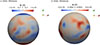Fig. 1. Snapshots of adopted initial magnetic-field map at the inner boundary. The sphere on the left represents the magnetic map for August 1, 2008 (the case of the solar minimum, where the dipole component is dominant), whereas the sphere on the right shows the magnetic map for March 9, 2016 (the case of the solar maximum).

5.1. The case of the solar minimum

This subsection presents the numerical results obtained for the solar-minimum case, the period of relatively lower solar activity in the solar cycle, during which transient phenomena such as sunspots and solar eruptions are at their lowest. In the numerical results, we emphasize physical quantities, such as velocity, temperature, and density contours for ions and neutrals, by making direct comparisons of the contour plots for “with-or-without” scenarios, along with the most apparent physical explanations, particularly when highlighting the effect of source-sink terms (S, Eq. (30)). Figure 2 shows the plot for ions’ radial velocity, V_ri, in Cases1, (a) and 2 (b). In Case 1 (a), V_ri follows a pronounced acceleration near the polar regions where it rises steeply to a peak value of approximately ≈ 140 km s⁻¹ at around 4–5 R_s. This peak value is consistent with slow-wind observations near these radial distances. Surrounding the central core region are smaller scale azimuthal lobes of elevated velocity superimposed on a broader background of moderately enhanced outflow. In Case 2 (b), the contour is nearly hydrostatic, where the contours are concentric and smoother than those visible in panel (a). Physically, in Case 1 (a), due to additional source-sink terms, the local ion temperature and pressure balance are modified. The presence of the empirical heating term of Eq. (33) injects energy mainly where the field lines are typically strong, i.e., near the coronal foot points. Additionally, thermal conduction (Braginskii 1965) transports energy along the field lines, where the heat remains trapped within closed loops, building up pressure and forming a dark petal-like shape around the white disk. Along the open flux, the heat escaped radially, lifting the ion’s V_ri outward with inflated surrounding layers (Fig. 2a). Additionally, near the Sun’s surface, gravitational forces dominate over the pressure gradient driven by heating. In the rest of the region, pressure gradient compensates over gravitational potential, leading to positive radial speeds (∼ 140 km s⁻¹).

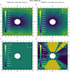Fig. 2. Contour plots of radial velocity of the ions Vri (a, b) and Vri − Vrn (c, d), with (a, c) and without (b, d) the source-sink term. All velocities are expressed in meters per second (m s−1). These plots correspond to the solar-minimum case.

In Case 2 (Fig. 2b), marked by suppressed thermal-energy accumulation, plasma species remain relatively quiescent. Here, the absence of heating implies that electromagnetic and gravitational forces nearly balance, and the plasma remains in a low-energy, nearly isothermal state. This results in the corona being characterized by relatively smoother, almost concentric contours with a symmetrical bubble-like structure as compared to Case 1. We also observe that the magnitude of the velocity in both cases is of the same order, comparable to magnitudes obtained in earlier work by Brchnelova et al. (2023) (see left panels in Fig. 7). This indicates that the ion outflow speed, initially super-Alfvénic, is primarily driven by large-scale expansion rather than local heating, radiative cooling, or conduction. The presence of such a local source term appears to affect the velocity distribution rather than its magnitude, suggesting that our heating term is relatively small. The critical conclusion drawn from the two cases is that the inclusion or omission of the source-sink term in the ion energy may provide the balance between plasma inflows and outflows. Gravitational force may drive plasma inflow, while thermal pressure and magnetic forces may drive plasma outflows. The empirical heating term (Eq. (33)) acts as a leading radial accelerator of coronal plasma and redistributes momentum laterally due to thermal conduction; such effects disappear once S = 0.

Figure 2 shows the contour plot for the ion-neutral radial-velocity drift, V_ri − V_rn, for Case 1 (c) and Case 2 (d). In Case 1, the values of V_ri − V_rn are relatively low, reaching a maximum of approximately 7 × 10² m s⁻¹, in contrast to the scenario where source-sink terms are turned off, where V_ri − V_rn is about ten times greater. Interpreting physically, the presence of explicit heating and cooling regulates the ions’ temperature and, therefore, moderates the ion pressure gradients. This reduces the differential acceleration between ions and neutrals, allowing the momentum-exchange terms to maintain strong coupling and suppress significant drift, thus yielding a relatively smoother spatial contour.

On the other hand, for Case 2 (d), the absence of the source-sink term leads to relatively weaker pressure support, while ions continue to accelerate under electromagnetic and gravitational forces. Neutrals, which do not experience magnetic stresses and evolve primarily through adiabatic expansion, cannot follow this enhanced ion acceleration. Even though the collisional momentum-exchange terms are unchanged, they do not compensate for the larger force imbalance, and the drift grows large. As a result, ions strongly decouple from neutrals and develop significant radial spikes emanating from the central cavity. Finally, the analysis of the obtained results highlights that thermodynamic source-sink terms may regulate the magnitude of the force imbalance between species. This imbalance may determine how effectively momentum exchange can maintain ion-neutral coupling over large coronal length scales.

The implemented source-sink terms can have a profound impact on the plasma’s overall thermodynamics, altering the mass-density structures of ions and neutrals. Figure 3 shows the contour plot of log𝜚_i (a, b) and neutrals log ϱ_n (c, d) for Case 1 (a, c) and Case 2 (b, d). For Case 1, both mass-density profiles (ions and neutrals) exhibit a bulging shape contour. Note that the contour in panel (a) demonstrates a relatively weaker radial stratification of 𝜚_i, where the inner corona is more inflated. In contrast, Case 2 maintains an almost spherical shape for both ions and neutrals, where 𝜚_i falls off more steeply with radius, producing a correspondingly steeper radial stratification. Interestingly, 𝜚_n contours (c, d) also follow a pattern similar to the contour profile of 𝜚_i in terms of the radial stratification. Physically, in Case 1, the injected heating raises the ion pressure, supporting the ion fluid against gravity and thereby maintaining a denser, more extended inner corona. In Case 2, by contrast, the plasma cools through adiabatic expansion, so the pressure support is weaker, and the ion mass density (𝜚_i) falls off more steeply with radius. As a result, the system approaches a state close to hydrostatic balance, where the dominant competing forces are the radial-pressure gradient and gravity. The implementation of the source-sink terms in our study yields an almost elliptical shape (a, c), in contrast with the nearly spherical symmetry observed in the neutral density plots across all cases in Brchnelova et al. (2023) (right panels in Fig. 7). Overall, the visible features in all the plots demonstrate the influence of including channelling proper local source-sink terms within the MF-MHD model regime. The inclusion of realistic heating, conduction, and radiative loss terms can transform the low corona from a nearly hydrostatic, partially ionized atmosphere into a more thermally driven, highly ionized outflow. Empirical source-sink terms lead to weak radial stratification, whereas their exclusion results in a steeper radial stratification.

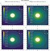Fig. 3. Contour plots of flow field of log 𝜚i (a, b) and log 𝜚n (c, d) with (a, c) and without a source term (b, d). The densities are expressed in kilograms per cubic meter (kg m−3). These plots correspond to the solar-minimum case.

Including the local source is expected to alter the plasma temperature. Figure 4 represents a contour plot corresponding to (log T_i, a, b) and temperature of neutrals (log T_n, c, d) in Case 1 (a, c) and Case 2 (b, d). The plots illustrate the thermal structure shape and the spatial features, which vary significantly between the two cases. Clearly, the panels (a) and (c) show similar, partially broad, reddish shells (∼1.3 − 1.6 MK) that fill the low corona, which is primarily located near the source and fades only gradually with radius. This is primarily due to the ions acquiring energy through the empirical heating term U_H, which remains deposited mainly below 2 R_s. However, parallel thermal conduction redistributes internal energy outward along the field lines, so the ions remain at a high temperature over a large volume. Optically thin radiative losses also play a key role, removing energy efficiently in the dense, low-corona region (Fig. 3), preventing runaway heating and helping establish a quasi-steady balance among heating, conduction, and radiation.

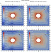Fig. 4. Contour plot of log Ti (a, b) and log Tn (c, d), with (a, c) and without (b, d) source-sink term. All temperatures are expressed in kelvin (K). These plots correspond to the solar-minimum case.

On the other hand, the contour plot corresponding to log T_n(c, d) retains a thin, hot rim right above the surface (red/orange regions), turning blue by r ∼  3 R_s. Note that the log T_n contours in both cases are similar to the respective log T_i counterpart (a, b). This is primarily because ions and neutrals are initialized with comparable temperatures, and the neutral-energy equation contains no source-sink terms or collisional-energy exchange; therefore, neutrals evolve essentially adiabatically in both cases. The presence of an additional source-sink term in the ion-energy equation perturbs the adiabatic background, modifying T_i (a, b) without drastically altering its morphology.

In summary, for the solar-minimum case, the presence of radiative cooling and empirical heating alters the corona’s structure. Case 1 shows a dynamic, higher-temperature corona with significant plasma outflow (≈ 100 km s⁻¹) and tight ion-neutral coupling, whereas Case 2 remains nearly static, cooler, and decoupled.

5.2. The case of the solar maximum

The solar maximum is the period characterized by a relatively high number of sunspots, indicating frequent solar activity. Figure 5 shows the contour plot of ion radial velocity ${\mathrm{V}}_{{\mathrm{r}}_{\mathrm{i}}}$ for Cases 1 (a) and 2 (b). A good contrast is visible in both scenarios, where the contour plot in panel (a) exhibits fan-shaped channels of outflow reaching ≈ 2 × 10⁵ m s⁻¹ (yellow region) and narrow wedges of spatial inflow lobes (dark/purple regions) down to ≈ −5.5 × 10^5.5 m s⁻¹ at high latitude. These intense, anisotropic flows arise where the strong, multipolar magnetic field concentrates the empirical heating and the associated pressure gradients into magnetic funnels above active regions. The steep pressure gradients along these funnels, together with the guiding effect of the magnetic field in the heated funnels, propel faster radial plasma outflows (∼ 2 × 10⁵ m s⁻¹) in the corresponding channels. However, the trend in Case 2 (b) reveals a gentler, ring-like flow, with weaker driving pressure gradients in the absence of source-sink terms, so the radial acceleration is reduced, and the flow pattern becomes more ring-like and symmetric, allowing the plasma to expand more adiabatically, slowly, and evenly than in the highly structured jets of Case 1.

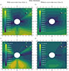Fig. 5. Contour plots of radial velocity of ions Vri (a, b) and Vri − Vrn (c, d), with (a, c) and without (b, d) the source-sink term. All velocities are expressed in the meter per second (m s−1). These plots here correspond to the case of the solar maximum.

The contour plots in Fig. 5 compare the ion-neutral velocity drift V_ri − V_rn, respectively, in Cases 1 (c) and 2 (d). The radial component of ion-neutral velocity drift (V_ri − V_rn) (c) with source-sink term shows substantial drift up to 10⁵ m s⁻¹ (yellow region) aligning with the outflow channels accompanied by negative drifts reaching ≈ 7 × 10⁴ m s⁻¹. The drift patterns during the solar maximum are driven by a strong, complex magnetic field, such as that found in active regions, which produces large electromagnetic forces that dominate the ion momentum balance. Consequently, the ions are rapidly driven outward, whereas neutrals, unaffected by the magnetic field, lag under the influence of gravity and collisional drag. As a result, a substantial velocity separation develops between the two species. We also observed a similarly large drift pattern in panel (d). This consistency suggests that during solar maximum, the overall magnetic activity is so intense compared to the source-sink term that whether these terms are included or not, ion and neutral flows decouple comparably in both cases, unlike in the case of the solar minimum (Fig. 2c, d).

Physically, regions of large drift correspond to where enhanced wave damping or frictional heating could occur. (Judge 2020; Wójcik et al. 2020; Martínez-Gómez et al. 2022). The unique patterns observed in Cases 1 and 2 illustrate how heating and cooling mechanisms within the plasma system affect the degree of coupling, decoupling, and spatial characteristics. Notably, heating during periods of intense solar activity does not lead to strong decoupling; instead, ions are accelerated considerably more than neutrals in both cases. Furthermore, the radial component of drift velocity is a critically important parameter for determining collisional coupling, i.e., where V_ri − V_rn is large, it is expected that there will be more exchange of momentum and energy (see Eqs. (9), (21), and (22)).

Figure 6 displays the log 𝜚_i (a, b) and neutrals log 𝜚_n (c, d) for Cases 1 (a, c) and 2 (b, d). Overall, the mass density profiles in all panels maintain roughly spherical contours, indicating that the large-scale stratification is primarily governed by gravity, pressure force, and the magnetic-field expansion rather than by additional source-sink terms. A modest contrast in terms of density scale height appears between panels (a) and (b). In Case 1, the additional source-sink terms increase the out-of-pressure and therefore the density scale height, producing a slightly weaker radial stratification and a mildly inflated inner-coronal region. Panel (a) shows a weak radial stratification with the mildly inflated inner-coronal region compared to panel (b). In Case 2, where the plasma cools primarily through the adiabatic expansion, 𝜚_i decreases more rapidly with radius, causing relatively steeper stratification. In contrast, the contour plot corresponding to neutral mass density (c, d) shows virtually no difference between the two cases. It is primarily because electromagnetic forcing during solar maximum strongly dominates the modest thermal effects included in Case 1. Since neutrals are not subject to electromagnetic forces and are not thermally coupled to ions in our model, their distribution is mainly governed by gravity and collisional drag. As a result, their density profiles remain nearly identical in both cases, implying that the source-sink term does not considerably affect the neutral density distribution in the event of solar maximum, as opposed to solar minima (Fig. 3). Essentially, these contour plots illustrate how the source-sink term in the energy equation determines the degree of plasma compression due to gravitational effects, thereby reconstructing the ion and neutral density fields within a multi-fluid MHD framework.

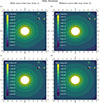Fig. 6. Contour plots of flow-field of log 𝜚i (a, b) and log 𝜚n (c, d), with (a, c) and without a source term (b, d). The densities are expressed in kilograms per cubic meter (kg m−3). These plots here correspond to the case of the solar maximum.

Figure 7 displays the log T_i (a, b), and log T_n (c, d), for Case 1 (a, c) and Case 2 (b, d). In Case 1, panel (a) reveals a narrow, irregular, highly localized funnel-shaped channel of very hot plasma (∼2.0 × 10⁶ K) guided along the magnetic-field lines. By contrast, panel (b) in Case 2 shows a more organized structure, where only a moderately hot layer develops close to the surface. The neutral temperatures in panels (c) and (d) exhibit smooth, concentric contours in both cases. It is primarily because the implemented source-sink terms do not directly influence the neutral component, and ion-neutral thermal coupling is absent in our model; therefore, their temperature evolution is primarily governed by gravity, adiabatic expansion, and weak collisional momentum coupling. As a result, the neutral temperature is primarily insensitive to whether the source-sink terms are included. Taken together, the results indicate that Case 1 produces a strongly heated ion corona with localized hot patches and steep temperature gradients, whereas Case 2 leads to a smoother and comparatively cooler atmosphere with gentler gradients. Overall, demonstrating that the thermodynamic modifications introduced by the source-sink terms primarily influence the ionized fluid during solar maximum.

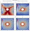Fig. 7. Contour plot of log Ti (a, b) and log Tn (c, d) with (a, c) and without (b, d) source-sink term. All temperatures are expressed in kelvin (K). These plots here correspond to the case of the solar maximum.

6. Source-sink terms and magnetic topology

Figure 8 displays four snapshots of the photosphere, highlighting the interplay between source-sink terms and solar activity in reshaping the radial magnetic field, B_r. The red and blue surface regions denote outward and inward magnetic flux, respectively, with the associated coronal field lines superimposed. Panels (a) and (b) correspond to a solar minimum for Case 1 and Case 2, while panels (c) and (d) depict the solar-maximum case. During solar minimum (a, b), the photospheric field is relatively unipolar, with large polar coronal holes and typically strong field near the coronal foot points, which aid thermal conduction (Braginskii 1965) in transporting energy along the field lines. In both cases, the field appears relatively smooth and dipolar on large scales. The source terms in Case 1 cause only minor local changes; for example, heating inflates a low-latitude flux tube, slightly distorting the northern polar hole. These effects do not strengthen the photospheric B in Case 1; instead, they redistribute the existing field by expanding magnetic cavities. During solar maximum (panels c and d), the field is highly complex, with many active regions (intermixed red and blue) and tangled open field lines. Here, the influence of the source terms is much less visible: the overall skeleton of field lines is dominated by the strong magnetic map, so the heated-cooled (Case 1) and adiabatic (Case 2) solutions differ only subtly. In short, Fig. 8 shows that heating can locally modify the coronal-field configuration (especially at solar minimum). Still, the global field topology is primarily set by the photospheric magnetogram.

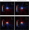Fig. 8. Snapshots of full two-fluid MHD COCONUT solution with source term (a, c) and without the source-sink term (b, d) for the solar minimum (a, b) and solar maximum (c, d). The simulated radial magnetic field, Br, is plotted on the solar surface.

7. Model performance

Implementing the new source-sink term is expected to impact the model’s performance and the solver’s speed, depending on the problem’s complexity and the stiffness of the implemented terms. This paper evaluates the model’s performance in terms of residual and wall-clock time. The residual of any physical quantity, f, in the numerical modelling, is defined as

$$\begin{array}{c}\hfill \mathrm{res}(f)=\log \sqrt{{\mathrm{\Sigma }}_i{(f_i^t-f_i^{t+1})}^2}.\end{array}$$(34)

Here, i and t denote the spatial and temporal indices, respectively. Since the multi-fluid equations are solved in dimensional form, the obtained residuals are in dimensional units, which can be converted to nondimensional form using the reference temperature T_ref = 2.3 × 10¹¹ K. Using Eq. (34),

$$\begin{array}{cc}\hfill \mathrm{res}(f^{\ast })& =\mathrm{res}(f)-log(2.3\times {10}^{11}),\hfill \end{array}$$(35)

$$\begin{array}{cc}\hfill \mathrm{res}(f^{\ast })& \approx \mathrm{res}(f^{)}-11.36.\hfill \end{array}$$(36)

Here, res(f^∗) is the residual of the physical quantity in the nondimensional form. If one reads that at the current iteration the residual in the nondimensional simulation quantity is −5, which means that the total sum of the changes in the flow-field quantity between two consecutive iterations is 10⁻⁵. This range of the residual value typically indicates a well-converged solution. Figure 9 compares the residual corresponding to T_i versus the number of iterations in the case of solar minimum (a) and in the case of solar maximum (b). In both panels, the blue curve represents the residual in Case 1, while the red curve represents Case 2. For the solar minimum (a), we find the residual at the end of the approximately 20 000^th iteration is roughly 4.8 (∼ − 6.56 in nondimensional form) in Case 1, while 3.5 (∼ − 7.86 in nondimensional form) in Case 2. Similarly, for solar maximum, we observe the obtained residuals of ∼3 (∼ − 8.36) in Case 1 and ∼2.6 (∼ − 8.76) in Case 2. These small quantities indicate the good convergence of the obtained steady-state solution. Moreover, we note that the simulations were performed using the COCONUT code’s implicit steady-state solver, with the interactive CFL number (Courant et al. 1928) controlling the time step. Because the time stepping is implicit and the CFL was adjusted during the run, while monitoring the status of the residual, as defined in Eq. (34), it may not decrease monotonically with each iteration, and this does not necessarily mean that the solution is diverging. When CFL is increased to accelerate convergence, the time step increases, so the change between consecutive iterations can temporarily grow, producing the bumps and mild increases, as clearly visible in Fig. 9. We also emphasize that implementing the additional source-sink terms is expected to stiffen the system; therefore, we must be more conservative when increasing the CFLs. Nevertheless, the final nondimensional residual (shown in Table 1) confirms that the flow field and solution are converged, even though the residual curves may not be strictly monotonically decreasing. Additionally, the plateau in the residual for the case of the solar minimum (with source-sink terms) indeed shows similar residual values as the simulation progresses in later phases, which shows that residuals can be similar per time step, but the time step becomes larger in later phases of the simulation.

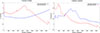Fig. 9. Variation of Ti residual with iteration count in the numerical simulation for the solar minimum (a) and solar maximum (b). The blue curve belongs to Case 1 (with source-sink term), whereas the red curve corresponds to Case 2 (without source-sink term).

Table 1 summarizes the computed residual values after simulating the solar minimum and solar maximum for the first hour (wall-clock time) corresponding to both cases. All numerical simulations were performed on a single node with two Xeon E5-2670 v3 CPUs @ 2.3 GHz (Haswell), 48 cores and 24 threads each, on the LUNAR cluster at UMCS Lublin, Poland. The first rows of both tables represent the residual for T_i, while the second rows represent the residual for ρ_i. We note that the residual for T_i varies in the range of −6 ∼ −8, while the residual for 𝜚_i varies in the range of −20 ∼ −22 in both cases. Upon comparing the obtained residual values in the table for both cases and residual trend in the plots in Fig. 9, it is evident that the residuals in both cases do not fluctuate considerably from each other and also lie in the typical range to support the converged solution. Based on the above result and the required time, we conclude that one can achieve the steady-state solution in a practical matter of time. Moreover, activating the new source-sink term requires only a little additional time and computational investment compared to the base model, making the model feasible for space-weather forecasting.

8. Summary and discussion

In this work, we extended the global two-fluid COCONUT coronal model by adding realistic source and sink terms to the ion energy equation. The source-sink terms include thermal conductivity, a radiative loss model for thin-plasma radiation, and empirical heating functions that represent the heating of the solar corona and scale with the magnetic-field strength. Physically, these terms describe the dominant thermodynamic processes thought to heat and cool the solar corona. Numerical simulations are conducted on real data-driven cases to investigate the impact of such terms on the dynamics of the solar coronal plasma during solar minimum (August 1, 2008) and maximum (March 9, 2016). The findings of our work underscore the need to incorporate such additional heating components into two-fluid MHD formulations to accurately define the ion and neutral dynamics of the lower corona in both solar maximum and minimum cases. The presented results reveal that it is essential to incorporate source-sink terms in calculations involving ion energy to equilibrate forces such as thermal pressure and gravity. This balance is crucial for the dynamics of plasma outflow and inflow in the solar atmosphere. The model is validated in terms of residual with and without the source-sink terms. The obtained results also indicate that the model can achieve steady-state solutions, making it a suitable option for space-weather forecasting.

This study introduced a mathematical framework to elucidate coronal dynamics in alignment with solar dynamical processes. However, the thermodynamic model of the corona may neglect the underlying physics of coronal heating and solar wind acceleration. Additionally, this research highlights its global scope. It may overlook small-scale phenomena, such as wave turbulence, nano-flares, and ion-neutral waves, which could be important for understanding solar dynamics. In addition, we modeled a global steady state and thus have not addressed time-dependent phenomena such as flares or coronal-mass ejections. A more extensive line of research involves linking the current model to another model, such as Icarus (Baratashvili et al. 2024), and validating the model’s predictions against observable data from solar missions. This would aid in assessing the model’s correctness, provide a quantitative description of the solar atmosphere, and improve the reliability of predicting space-weather phenomena. Such work is devoted to future projects. Moreover, future work should adopt a more realistic γ = 5/3 to accurately model the solar corona.

Finally, our refined two-fluid model suggests that accurately simulating the thermodynamics of the corona requires accounting for radiative losses, heat conduction, and heating that depends on magnetic fields. They result in a hot, organized corona and initiate realistic solar wind outflows under both quiet and active conditions. Omitting them may result in a purely hydrostatic corona. Therefore, for any comprehensive coronal model, particularly in the context of space-weather prediction, it is crucial to incorporate such elements to ensure physical relevance.

Acknowledgments

This work was carried out as part of the Space Weather Awareness Training Network (SWATNet) project, funded by the European Union’s Horizon 2020 research and innovation program under grant agreement No 955620. Views and opinions expressed are, however, those of the author(s) only and do not necessarily reflect those of the European Union or the European Research Council. Neither the European Union nor the granting authority is responsible for them. M. Kumar gratefully acknowledges the scholarship received from the Polish National Agency of Academic Exchange (NAWA) under the framework of the Uniwersytet Marii Curie-Skłodowskiej (UMCS) Doctoral Schools – Your Success in a Globalized World of Science to support the present work further. KM’s work was done within the framework of the project from the Polish Science Center (NCN) Grant No. 2020/37/B/ST9/00184. Numerical simulations were run on the LUNAR cluster at the Institute of Mathematics at UMCS in Lublin, Poland. The authors express gratitude to the anonymous referee for their insightful comments and suggestions. SP is funded by the European Union (ERC, Open SESAME, 101141362). These results were also obtained in the framework of the projects C16/24/010 (C1 project Internal Funds KU Leuven), G0B5823N and G002523N (WEAVE) (FWO-Vlaanderen), and 4000145223 (SIDC Data Exploitation (SIDEX2), ESA Prodex).

References

All Tables

All Figures

	Fig. 1. Snapshots of adopted initial magnetic-field map at the inner boundary. The sphere on the left represents the magnetic map for August 1, 2008 (the case of the solar minimum, where the dipole component is dominant), whereas the sphere on the right shows the magnetic map for March 9, 2016 (the case of the solar maximum).
In the text

	Fig. 2. Contour plots of radial velocity of the ions Vri (a, b) and Vri − Vrn (c, d), with (a, c) and without (b, d) the source-sink term. All velocities are expressed in meters per second (m s−1). These plots correspond to the solar-minimum case.
In the text

	Fig. 3. Contour plots of flow field of log 𝜚i (a, b) and log 𝜚n (c, d) with (a, c) and without a source term (b, d). The densities are expressed in kilograms per cubic meter (kg m−3). These plots correspond to the solar-minimum case.
In the text

	Fig. 4. Contour plot of log Ti (a, b) and log Tn (c, d), with (a, c) and without (b, d) source-sink term. All temperatures are expressed in kelvin (K). These plots correspond to the solar-minimum case.
In the text

	Fig. 5. Contour plots of radial velocity of ions Vri (a, b) and Vri − Vrn (c, d), with (a, c) and without (b, d) the source-sink term. All velocities are expressed in the meter per second (m s−1). These plots here correspond to the case of the solar maximum.
In the text

	Fig. 6. Contour plots of flow-field of log 𝜚i (a, b) and log 𝜚n (c, d), with (a, c) and without a source term (b, d). The densities are expressed in kilograms per cubic meter (kg m−3). These plots here correspond to the case of the solar maximum.
In the text

	Fig. 7. Contour plot of log Ti (a, b) and log Tn (c, d) with (a, c) and without (b, d) source-sink term. All temperatures are expressed in kelvin (K). These plots here correspond to the case of the solar maximum.
In the text

	Fig. 8. Snapshots of full two-fluid MHD COCONUT solution with source term (a, c) and without the source-sink term (b, d) for the solar minimum (a, b) and solar maximum (c, d). The simulated radial magnetic field, Br, is plotted on the solar surface.
In the text

	Fig. 9. Variation of Ti residual with iteration count in the numerical simulation for the solar minimum (a) and solar maximum (b). The blue curve belongs to Case 1 (with source-sink term), whereas the red curve corresponds to Case 2 (without source-sink term).
In the text

References

- Andretta, V., & Jones, H. P. 1997, ApJ, 489, 375 [NASA ADS] [CrossRef] [Google Scholar]
- Aschwanden, M. J. 2019, New Millennium Solar Physics (Springer), 458 [Google Scholar]
- Aslanyan, V., Meyer, K. A., Scott, R. B., & Yeates, A. R. 2024, ApJ, 961, L3 [Google Scholar]
- Baratashvili, T., Brchnelova, M., Linan, L., Lani, A., & Poedts, S. 2024, ArXiv e-prints [arXiv:2407.17903] [Google Scholar]
- Bose, S., De Pontieu, B., Hansteen, V., et al. 2024, Nat. Astron, 8, 697 [Google Scholar]
- Braginskii, S. 1965, Rev. Mod. Plasma Phys., 1, 205 [Google Scholar]
- Braileanu, B. P., Lukin, V., Khomenko, E., & De Vicente, Á. 2019, A&A, 627, A25 [NASA ADS] [CrossRef] [EDP Sciences] [Google Scholar]
- Brchnelova, M., Zhang, F., Leitner, P., et al. 2022, JPP, 88, 905880205 [Google Scholar]
- Brchnelova, M., Kuźma, B., Zhang, F., Lani, A., & Poedts, S. 2023, A&A, 678, A117 [NASA ADS] [CrossRef] [EDP Sciences] [Google Scholar]
- Browning, P. 1991, PPCF, 33, 539 [Google Scholar]
- Califano, F. 2000, AIP Conf. Proc., 537, 126 [Google Scholar]
- Cargill, P. J. 2000, ASR, 26, 1759 [Google Scholar]
- Courant, R., Friedrichs, K., & Lewy, H. 1928, Math. Ann., 100, 32 [Google Scholar]
- De Moortel, I., & Browning, P. 2015, Phil. Trans. R. Soc. A, 373, 20140269 [Google Scholar]
- Dedner, A., Kemm, F., Kröner, D., et al. 2002, J. Comput. Phys, 175, 645 [NASA ADS] [CrossRef] [Google Scholar]
- Dorotovic, I., Lukác, B., Minarovjech, M., & Rybanskỳ, M. 1997, Theoretical and Observational Problems Related to Solar Eclipses (Springer), 189 [Google Scholar]
- Downs, C., Roussev, I. I., van der Holst, B., et al. 2010, ApJ, 712, 1219 [CrossRef] [Google Scholar]
- Downs, C., Warmuth, A., Long, D. M., et al. 2021, ApJ, 911, 118 [CrossRef] [Google Scholar]
- Einaudi, G., & Velli, M. 2005, ASP: Proceedings of the Seventh European Meeting on Solar Physics, Catania, Italy, 11–15 May 1993 (Springer), 147 [Google Scholar]
- Feng, X. 2019, Magnetohydrodynamic Modeling of the Solar Corona and Heliosphere (Springer) [Google Scholar]
- Fontenla, J., Avrett, E., & Loeser, R. 1993, ApJ, 406, 319 [NASA ADS] [CrossRef] [Google Scholar]
- Goedbloed, H., Keppens, R., & Poedts, S. 2019, MHD of Laboratory and Astrophysical Plasmas [Google Scholar]
- Gombosi, T. I., van der Holst, B., Manchester, W. B., & Sokolov, I. V. 2018, Liv. Rev. Sol. Phys., 15, 1 [NASA ADS] [CrossRef] [Google Scholar]
- Gopalswamy, N. 2022, Atmosphere, 13, 1781 [CrossRef] [Google Scholar]
- Gronenschild, E. H. B. M., & Mewe, R. 1978, A&AS, 32, 283 [NASA ADS] [Google Scholar]
- Hu, Y., Feng, X., Wu, S., & Song, W. 2008, JGR: Space Phys., 113 [Google Scholar]
- Iijima, H., Matsumoto, T., Hotta, H., & Imada, S. 2023, ApJ, 951, L47 [NASA ADS] [CrossRef] [Google Scholar]
- Jin, M., Schrijver, C., Cheung, M., et al. 2016, ApJ, 820, 16 [NASA ADS] [CrossRef] [Google Scholar]
- Judge, P. G. 2020, MNRAS, 498, 2018 [Google Scholar]
- Khomenko, E., Lukin, V., & Popescu Braileanu, B. 2021, 43rd COSPAR Scientific Assembly. Held 28 January– 4 February, 43, 976 [Google Scholar]
- Klimchuk, J. A. 2006, Sol. Phys, 234, 41 [Google Scholar]
- Kuperus, M., Ionson, J. A., & Spicer, D. S. 1981, ARA&A, 19, 7 [Google Scholar]
- Kuźma, B., Brchnelova, M., Perri, B., et al. 2023, ApJ, 942, 31 [CrossRef] [Google Scholar]
- Lani, A., Quintino, T., Kimpe, D., et al. 2005, Computational Science-ICCS 2005: 5th International Conference, Atlanta, GA, USA, May 22–25, 2005 (Springer), 279 [Google Scholar]
- Lionello, R., Linker, J. A., & Mikić, Z. 2008, ApJ, 690, 902 [Google Scholar]
- Lu, Z., Chen, F., Ding, M., et al. 2024, Nat. Astron, 1 [Google Scholar]
- Martínez-Gómez, D., Oliver, R., Khomenko, E., & Collados, M. 2022, ApJ, 940, L47 [CrossRef] [Google Scholar]
- Martínez-Sykora, J., De Pontieu, B., Hansteen, V., & Carlsson, M. 2015, Phil. Trans. R. Soc. A: Math. Phys. Eng. Sci., 373, 20140268 [Google Scholar]
- Meier, E., & Shumlak, U. 2012, PoP, 19 [Google Scholar]
- Melis, L., Soler, R., & Ballester, J. L. 2021, A&A, 650, A45 [NASA ADS] [CrossRef] [EDP Sciences] [Google Scholar]
- Mikić, Z., Linker, J. A., Schnack, D. D., Lionello, R., & Tarditi, A. 1999, PoP, 6, 2217 [Google Scholar]
- Nahar, S. N. 2021, Atoms, 9, 73 [NASA ADS] [CrossRef] [Google Scholar]
- Pagano, P., Bemporad, A., & Mackay, D. H. 2020, A&A, 637, A49 [NASA ADS] [CrossRef] [EDP Sciences] [Google Scholar]
- Parnell, C. E., & De Moortel, I. 2012, Phil. Trans. R. Soc. A: Math. Phys. Eng. Sci., 370, 3217 [Google Scholar]
- Perri, B., Leitner, P., Brchnelova, M., et al. 2022, ApJ, 936, 19 [NASA ADS] [CrossRef] [Google Scholar]
- Perri, B., Kuźma, B., Brchnelova, M., et al. 2023, ApJ, 943, 124 [NASA ADS] [CrossRef] [Google Scholar]
- Pevtsov, A. A., Fisher, G. H., Acton, L. W., et al. 2003, ApJ, 598, 1387 [Google Scholar]
- Poedts, S. 2019, PPCF, 61, 014011 [Google Scholar]
- Poedts, S., Kochanov, A., Lani, A., et al. 2020a, JSWSC, 10, 14 [Google Scholar]
- Poedts, S., Lani, A., Scolini, C., et al. 2020b, JSWSC, 10, 57 [Google Scholar]
- Riley, P., Linker, J., & Mikić, Z. 2001, JGR: Space Phys., 106, 15889 [Google Scholar]
- Rosner, R., Tucker, W. H., & Vaiana, G. 1978, ApJ, 220, 643 [NASA ADS] [CrossRef] [Google Scholar]
- Sakurai, T. 2017, Proc. Jpn. Acad. Ser. B, 93, 87 [Google Scholar]
- Schmelz, J., & Winebarger, A. 2015, Phil. Trans. R. Soc. A: Math. Phys. Eng. Sci., 373, 20140257 [Google Scholar]
- Schnack, D. 1994, Structure and Dynamics of the Solar Corona, Tech. rep [Google Scholar]
- Sime, D., & McCabe, M. 1990, Sol. Phys, 126, 267 [Google Scholar]
- Soler, R., & Ballester, J. L. 2022, Front. Astron. Space Sci, 9, 789083 [Google Scholar]
- Tu, C.-Y., & Marsch, E. 1997, Sol. Phys, 171, 363 [Google Scholar]
- Usmanov, A. V., & Goldstein, M. L. 2003, AIP Conf. Proc., 679, 393 [NASA ADS] [CrossRef] [Google Scholar]
- Van Doorsselaere, T., Srivastava, A. K., Antolin, P., et al. 2020, SSR, 216, 1 [Google Scholar]
- Venkatakrishnan, V. 1993, 31st Aerospace Sciences Meeting, 880 [Google Scholar]
- Vial, J.-C., & Chane-Yook, M. 2016, Sol. Phys, 291, 3549 [Google Scholar]
- Voronov, G. S. 1997, At. Data Nucl. Data Tables, 65, 1 [Google Scholar]
- Wang, Y.-M., & Sheeley, N., Jr. 1990, ApJ., 355, 726 [Google Scholar]
- Wargnier, Q., Martinez-Sykora, J., Hansteen, V. H., & De Pontieu, B. 2022, ApJ, 933, 205 [NASA ADS] [CrossRef] [Google Scholar]
- Wójcik, D., Kuźma, B., Murawski, K., & Musielak, Z. 2020, A&A, 635, A28 [NASA ADS] [CrossRef] [EDP Sciences] [Google Scholar]
- Yalim, M. S., Abeele, D. V., Lani, A., Quintino, T., & Deconinck, H. 2011, J. Comput. Phys, 230, 6136 [Google Scholar]
- Zaqarashvili, T., Khodachenko, M., & Rucker, H. 2011, A&A, 534, A93 [NASA ADS] [CrossRef] [EDP Sciences] [Google Scholar]
All Tables
Summary of obtained residual (nondimensional) in the initial one-hour (clock-wall time) run of the numerical simulation for the multi-fluid simulation for the variables (Ti, 𝜚i), in the cases of the solar minimum (a) and the solar maximum (b).