| Issue |
A&A
Volume 707, March 2026
|
|
|---|---|---|
| Article Number | A119 | |
| Number of page(s) | 10 | |
| Section | Stellar structure and evolution | |
| DOI | https://doi.org/10.1051/0004-6361/202557374 | |
| Published online | 02 March 2026 | |
Asteroseismology and buoyancy glitch inversion with Fourier spectra of gravity mode period spacings
Institute of Astronomy (IvS), Department of Physics and Astronomy, KU Leuven Celestijnenlaan 200D 3001 Leuven, Belgium
★ Corresponding author: This email address is being protected from spambots. You need JavaScript enabled to view it.
Received:
23
September
2025
Accepted:
6
November
2025
Abstract
Aims. We investigated the small, quasi-periodic modulations seen in the gravity-mode period spacings (ΔPk) of pulsating stars. These “wiggles” are produced by buoyancy glitches - sharp features in the buoyancy frequency (N) caused by composition transitions and the convective–radiative interface.
Methods. We computed the Fourier transform of the period-spacing series, FT(ΔPk), as a function of radial order k. We show that FT(ΔPk) traces the radial derivative of the normalized glitch profile δN/N with respect to the normalized buoyancy radius; peaks in FT(ΔPk) therefore pinpoint jump/drop locations in N and measure their sharpness. We also note that the Fourier transform of relative period perturbations (deviations from asymptotic values), FT(δP/P), directly recovers the absolute value of the glitch profile |δN/N|, enabling a straightforward inversion for the internal structure.
Results. The dominant FT(ΔPk) frequency correlates tightly with the central hydrogen abundance (Xc), and thus with stellar age, for slowly pulsating B-stars, with only weak mass dependence. Applying the technique to Modules for Experiments in Stellar Astrophysics (MESA) stellar models and to observed slowly pulsating B-stars and γ Dor pulsators, we find typical glitch amplitudes δN/N ≲ 0.01 and derivative magnitudes ≲0.1, concentrated at chemical gradients and the convective boundary. This approach enables fast, ensemble asteroseismology of g-mode pulsators, constrains internal mixing and ages, and can be extended to other classes of pulsators, with potential links to tidal interactions in binaries.
Key words: waves / stars: evolution / stars: interiors / stars: oscillations
Current: Department of Applied Mathematics, School of Mathematics, University of Leeds, Leeds LS2 9JT, UK.
© The Authors 2026
 Open Access article, published by EDP Sciences, under the terms of the Creative Commons Attribution License (https://creativecommons.org/licenses/by/4.0), which permits unrestricted use, distribution, and reproduction in any medium, provided the original work is properly cited.
This article is published in open access under the Subscribe to Open model. This email address is being protected from spambots. You need JavaScript enabled to view it. to support open access publication.
1. Introduction
Stars, which are self-gravitating fluids (plasmas), mostly contain stratified regions that are capable of supporting internal gravity waves (Sutherland 2010). In these regions, buoyancy acts as the restoring force (Turner 1973), enabling gravity waves to propagate and form normal modes (g modes), thereby permitting direct probing of the deep stellar interior. In the asymptotic limit, high-order g modes form nearly uniformly spaced sequences in pulsation periods (Tassoul 1980), with a characteristic asymptotic period spacing that depends sensitively on the integral of the Brunt-Väisälä frequency (buoyancy frequency) through the propagation cavity.
Local sharp features such as the base of the convective envelope, He II ionization zone, and the convective-core boundary can act as glitches in acoustic modes and induce variations in the small frequency separation (Roxburgh & Vorontsov 1994; Basu 1997). Similarly, buoyancy glitches, such as composition-transition regions, can lead to deviations from the regular period-spacing pattern. Investigating these glitch-induced seismic signatures enables direct access to sharp structural features and mixing processes in the stellar interior (Cunha et al. 2024).
Observationally, gravity-mode period-spacing patterns have been detected across a wide range of pulsating stars. For γ Doradus stars, Kepler photometry revealed clear g-mode sequences, such as those in KIC 11145123 (Kurtz et al. 2014) and 611 stars in Li et al. (2019). Slowly pulsating B (SPB) stars extend this diagnostic to higher masses: Degroote et al. (2010) discovered that period spacing deviates from a uniform spacing; Pápics et al. (2014, 2015) reported period spacings in SPBs KIC 10526294 and KIC 7760680, followed by detailed seismic modeling by Moravveji et al. (2015, 2016). Pedersen et al. (2018, 2021) performed detailed seismic modeling to infer mixing profiles for 26 SPB systems. Similar modeling work includes Wu et al. (2018, 2020) and Szewczuk & Daszyńska-Daszkiewicz (2018). Shi et al. (2023) identified 286 new SPB candidates using Transiting Exoplanet Survey Satellite (TESS), Large Sky Area Multi-Object Fiber Spectroscopic Telescope (LAMOST), and Gaia surveys.
Compact pulsators such as white dwarfs (Althaus et al. 2010; Córsico et al. 2019) and subdwarf B (sdB) stars also exhibit g modes (Brassard et al. 1992; Charpinet et al. 2000; Uzundag et al. 2017; Guyot et al. 2025). Recent analyses of buoyancy glitches in sdB stars are presented in Cunha et al. (2024). Red giant stars (Mosser et al. 2014; Cunha et al. 2019; Ong et al. 2021) also exhibit mixed-character gravity modes.
Theoretical studies of g-mode pulsation periods have focused on incorporating rotational effects via the traditional approximation of rotation (Townsend & Teitler 2013; Bouabid et al. 2013), accounting for centrifugal deformation (Henneco et al. 2021), and magnetic fields (Rui et al. 2024; Lignières et al. 2024).
Wu et al. (2018) used the Fourier transform to study oscillatory signatures in period-spacing patterns, finding a tight relation between the frequency of variation, fΔP, and the central hydrogen fraction, Xc. A diagram (fΔP vs. Π0) analogous to the classical C–D diagram (Δν vs. δν02) for acoustic modes in solar-like oscillators was constructed (Christensen-Dalsgaard 1988). Zhang et al. (2023) and Hatta (2023) studied the prescribed buoyancy-glitch expressions and the induced period spacing variations.
Inspired by Wu et al. (2018), we extend the work of Miglio et al. (2008) and Zhang et al. (2023) and demonstrate that the Fourier spectrum of the gravity-mode period spacings, FT(ΔPk), can be used to probe the Brunt–Väisälä (Brunt for short) profile jump or drop points and to reconstruct the buoyancy glitch profile. We demonstrate the advantage of the buoyancy coordinate in Sect. 2. We derive the theoretical expressions that link the Fourier spectra of period spacings to the derivatives of the Brunt glitch profile in Sect. 3. These expressions are verified with MESA stellar models in Sect. 4. We discuss the effects of overshooting and mixing on the period spacing in Sect. 5, and the effect of rotation in Sect. 6. We then apply the method to observed g modes in SPB and γ Dor stars in Sect. 7. We conclude in Sect. 8.
2. Gravity mode period spacing and buoyancy coordinate
In fluids with density stratification, a vertically displaced parcel oscillates at the Brunt Väisälä (buoyancy) frequency,  . In regions with N2 > 0, where gravity waves propagate, buoyancy acts as the restoring force of the oscillation. In contrast, in convectively unstable regions with N2 < 0, gravity modes are evanescent.
Figure 1 (left column) presents the Brunt profile, N (in units of G = M = R = 1), as a function of the radial coordinate, x = r/R, for an M = 3.2 M⊙ main-sequence stellar structure model from MESA (Paxton et al. 2011, 2013). We adopted the “gs98” chemical composition and solar metallicity. We employed the Ledoux criterion for convection instability and used exponential convective core overshooting (Herwig 2000).
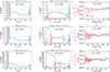 |
Fig. 1. Brunt–Väisälä (buoyancy) profiles, period spacings and their Fourier spectra for an M = 3.2 M⊙ MESA stellar model. Profiles are plotted as a function of the radial coordinate x = r/R (left panels) and the buoyancy coordinate, u (middle panels), with solar metallicity and convective overshooting, fov = 0.015. The hydrogen mass fraction, X, is shown by dashed green lines (multiplied by 10 for clarity). The gray-shaded regions denote the receding convective core. The dipole gravity-mode period spacings, ΔPk, are shown in the right panels, and their Fourier amplitude spectra, FT(ΔP), are overplotted in the middle panels (red lines, with super-Nyquist components in gray). The dominant Fourier-spectrum peak aligns with the sharp drop points of the Brunt profile and is labeled as uμ in red. |
As the star evolves on the main sequence, with central hydrogen depleting from Xc = 0.6 to Xc = 0.2, the convective core (where N ≈ 0, indicated by the gray-shaded regions to the left of the Brunt profile) recedes and leaves a chemical composition gradient region. Dashed green lines show the hydrogen mass fraction, X.
It is convenient to use the buoyancy coordinate, u (the normalized buoyancy radius), rather than the radial coordinate, x = r/R, since g modes are naturally described by their buoyancy travel time. In this coordinate, nodes of high-order g-modes are evenly spaced, with u defined as
 (1)
(1)
where, x1 is the inner boundary of the g-mode cavity. The two differential elements, du and dx, are related by
 (2)
(2)
which shows that du is proportional to the buoyancy travel time across dx, with the gravity-wave group velocity being  .
.
Using the u coordinate “stretches” the deep interior of the star and “compresses” the outer parts, so that the g-mode cavity resembles an almost constant slab of unit length, making structural diagnostics and glitches easier to identify.
Figure 1 (middle column) shows the Brunt profile in the u coordinate for SPB star models at different main-sequence stages, Xc = 0.6, 0.4, and 0.2. It is easier to see that, as the star evolves, the Brunt-profile bump shifts to the right, and its amplitude increases.
In regions where N/r is large (e.g., near a sharp composition gradient at the convective-core boundary), a small change in x produces a large jump in u. These regions act as glitches for gravity waves, which induce a variation in the g-mode period spacings. Mode nodes also cluster in high-N zones (mode trapping), especially in compact pulsators such as sdB stars and white dwarfs.
With a smooth Brunt profile, the pulsations of gravity modes observed in γ Dor and SPB stars are equally spaced in periods (Tassoul 1980). The asymptotic period spacing is  , where Π0 = 2π2(∫N2 > 0(N/r)dr)−1, which measures the “buoyancy travel time” across the g-mode cavity where N2 > 0.
Thus, the pulsation periods are well approximated by the linear relation (Van Reeth et al. 2016)
 (3)
(3)
where k is the radial order of the mode and k0 is a constant close to 0.5. The constant k0 may also absorb an additional constant due to phase offset and mode misidentification of the radial order, k. For Fourier analysis, k0 can be conveniently adjusted by an additive constant. When rotation is included in the traditional approximation, the expression remains unchanged except that  (see Sect. 6).
Figure 1 (right column) confirms that the equally spaced periods of g modes in the SPB model, with l = 1 and m = 0, oscillate around the asymptotic period spacing, Πl (dashed blue lines).
In reality, stellar interiors often contain sharp features relative to the wavelength of the gravity waves in question. This is particularly true for the convective-core boundary and composition-transition points, where the chemical abundances and therefore N undergo abrupt changes. In the left and middle columns of Figure 1, the hydrogen mass fraction, X (dashed green lines), shows sharp drops at the chemical composition transition region, which is the main source of the Brunt profile changes.
It is well known that a sharp drop in N produces a periodic variation in the g-mode period spacings, ΔP. In particular, the variation period in ΔP, measured in radial order k and denoted Δk, equals the reciprocal of the buoyancy radius at the chemical composition glitch, uμ (Miglio et al. 2008; Wu et al. 2018),
 (4)
(4)
The peak of the Fourier spectrum of the period spacings, FT(ΔPk) (red lines in the middle column of Figure 1), aligns with uμ, where N drops sharply. For the model with Xc = 0.6, uμ is about 0.1, as seen in the middle panel, implying a variation period in ΔP of about 10 radial orders (Δk ≈ 10). All Fourier spectra were calculated with radial orders from 9 to 125. Since the Nyquist frequency is 0.5, the Fourier spectra show a super-Nyquist reflection around this value.
The receding convective core leaves behind a chemical composition gradient region, as indicated by the increasing segments of the green lines, which gives rise to the expanding Brunt profile bump, N (middle column of Figure 1). As the star evolves from Xc = 0.6 to Xc = 0.2, the Brunt profile bump widens and uμ shifts to larger values, producing increasingly higher frequency variations in ΔP (Figure 1, right panel). The variation periods change from Δk ≈ 10 to ≈4, and ≈2.5 for Xc = 0.6, 0.4, and 0.2, respectively. For Xc = 0.2, the dominant variation frequency is very high, so consecutive peaks and troughs are very close. Visually, the subdominant low-frequency variation can be seen more easily, with the dip at k ≈ 110.
This concurrently increases the integral of N/r, thereby reducing the asymptotic period spacing, Πl, (from 5649 sec at Xc = 0.6 to 5000 sec at Xc = 0.2).
The sharply increasing part of N also generates a peak in FT(ΔPk) near u = 0, but this peak typically has a lower amplitude than the peak at uμ. This explains the slowly varying trend of the period spacing,ΔPk, observed in the right panels of Figure 1, particularly for the Xc = 0.4 and 0.2 models.
In the following sections, we take a step further and demonstrate that the Fourier spectra of the period spacings are directly linked to the Brunt glitch profile and its derivatives.
3. Connecting buoyancy glitch profile derivatives to Fourier spectra of period spacings
For gravity modes observed in intermediate- and high-mass stars, N changes sharply at the chemical composition gradient region near the convective-core boundary. Such buoyancy glitches, δN, induce a frequency perturbation, δω, which, when expressed as the relative pulsation-period perturbation at radial order k, takes the form (Montgomery et al. 2003; Miglio et al. 2008; Zhang et al. 2023)
![Mathematical equation: $$ \begin{aligned} \frac{\delta P_k}{P_k} \approx - \int ^1_0{\frac{\delta N(u)}{N(u)}[1+\sin (2\pi (k+k_0) u)]\mathrm{d}u}, \end{aligned} $$](/articles/aa/full_html/2026/03/aa57374-25/aa57374-25-eq9.gif) (5)
(5)
where N is the Brunt profile, and we define z(u) as z(u) = δN/N.
The observed pulsation periods of g modes are
 (6)
(6)
It is common to represent the period spacing at the k-th radial order, ΔPk, obs, as a function of the periods, Pk. By applying Eq. (3), one can easily recast this dependence in terms of the radial order k as follows:
 (7)
(7)
The above equation indicates that the period spacing, ΔPk, obs, is approximately a constant, a, with a small perturbation arising from dδPk/dk.
Starting from Eq. (5) and treating the term in the brackets [] as the derivative of C(u) = u − cos[2π(k + k0)u]/(2π(k + k0)), we integrate by parts to obtain
![Mathematical equation: $$ \begin{aligned} \delta P_k/P_k =+ \int ^1_0{z\prime (u)[u-\cos [2\pi (k+k_0) u]/(2 \pi (k+k_0))]\mathrm{d}u}. \end{aligned} $$](/articles/aa/full_html/2026/03/aa57374-25/aa57374-25-eq12.gif) (8)
(8)
The boundary terms vanish because it is natural to assume that Brunt glitch profiles in stars satisfy z(u = 0) = 0 and z(u = 1) = 01. Here, we denote z′(u) = dz/du. Multiplying by Pk and applying Eq. (3), we obtain
![Mathematical equation: $$ \begin{aligned} \delta P_k = a \int ^1_0{z\prime (u)[u (k+k_0)-\cos [2\pi (k+k_0) u]/(2 \pi )]\mathrm{d}u}. \end{aligned} $$](/articles/aa/full_html/2026/03/aa57374-25/aa57374-25-eq13.gif) (9)
(9)
Taking the derivative with respect to k on both sides, we obtain
/(2 \pi )]\mathrm{d}u}. \end{aligned} $$](/articles/aa/full_html/2026/03/aa57374-25/aa57374-25-eq14.gif) (10)
(10)
Thus, we can rewrite the observed period spacing as
![Mathematical equation: $$ \begin{aligned} \Delta P_{k,\mathrm{obs}}&\approx a + a \int ^1_0{z\prime (u)u [1 + \sin [2\pi (k+k_0) u]]\mathrm{d}u} \end{aligned} $$](/articles/aa/full_html/2026/03/aa57374-25/aa57374-25-eq15.gif) (11)
(11)
![Mathematical equation: $$ \begin{aligned}&=a + a \int ^1_0 z\prime (u)u \mathrm{d}u + a \int ^1_0[ z\prime (u) u \frac{e^{i 2 \pi (k+k_0) u}-e^{-i 2 \pi (k+k_0) u}}{2i} ]\mathrm{d}u \end{aligned} $$](/articles/aa/full_html/2026/03/aa57374-25/aa57374-25-eq16.gif) (12)
(12)
![Mathematical equation: $$ \begin{aligned}&=a - a \int ^1_0 z(u) \mathrm{d}u + a \int ^1_0[ z\mathrm{d}(u) u \frac{e^{i 2 \pi (k+k_0) u}-e^{-i 2 \pi (k+k_0) u}}{2i} ]\mathrm{d}u. \end{aligned} $$](/articles/aa/full_html/2026/03/aa57374-25/aa57374-25-eq17.gif) (13)
(13)
The second term is a negligible constant. Therefore, we have
![Mathematical equation: $$ \begin{aligned} f(k) = \frac{\Delta P_{k,\mathrm{obs}} - a}{a} \approx \int ^1_0 \frac{z\prime (u) u}{2 i}[ e^{i 2 \pi (k+k_0) u}-e^{-i 2 \pi (k+k_0) u} ]\mathrm{d}u. \end{aligned} $$](/articles/aa/full_html/2026/03/aa57374-25/aa57374-25-eq18.gif) (14)
(14)
Taking the Fourier transform with respect to k and transforming to the “frequency” space ξ on both sides gives
 (15)
(15)
![Mathematical equation: $$ \begin{aligned}&= \int ^{+\infty }_{-\infty } \left(\int ^1_0 \frac{z\prime (u) u}{2 i}[ e^{i 2 \pi (k+k_0) u}-e^{-i 2 \pi (k+k_0) u} ]\mathrm{d}u\right)e^{-i 2 \pi \xi k} \mathrm{d}k \end{aligned} $$](/articles/aa/full_html/2026/03/aa57374-25/aa57374-25-eq20.gif) (16)
(16)
 (17)
(17)
 (18)
(18)
The one-sided Fourier amplitude spectrum (denoted by “FT”) of ΔPk, obs is
 (19)
(19)
with  .
.
Since an extra ξ term appears in front of the derivative, dz/dξ, the near-zero peaks in FT(ΔPk) are strongly suppressed. This explains why the low-frequency peak is typically smaller than the dominant peak at the sharp drops in the Brunt profile uμ (e.g., Figure 1, middle panels).
The same derivation can be applied to the relative period perturbation  , yielding
 (20)
(20)
Thus, the one-sided Fourier amplitude spectrum is
 (21)
(21)
In practice, k (interpreted as “time”) is an integer and ℱ(ΔPk) is the discrete Fourier transform which transforms k to the ξ (“frequency”) space ranging from −0.5 to 0.5, with 0.5 being the Nyquist frequency. The variable u ranges from 0 to 1, and it is convenient to use u as the corresponding frequency space instead of ξ once the 0.5 offset has been accounted for.
Observationally, the two Fourier spectra are related by
 (22)
(22)
Since FT(ΔPk) and FT(δP/P) depend only on the glitch profile, z = δN/N, there is no dependence on the mode spherical degree, l. The observed period spacings for different l should exhibit variations with the same periodicity.
We verify the expressions derived above in Sect. 4.
Thus, the peaks in the Fourier spectra of the period spacings align with the locations where dz/du peaks, which typically correspond to sharp drops, dips and jumps, or kinks in the Brunt profile. The height of the peaks reflects the amplitude of the Brunt glitch derivative.
Once the glitch profile z(u) = δN/N is obtained, we can further recover the Brunt profile in physical coordinates, x = r/R. Rearranging Equation (2), we obtain
 (23)
(23)
Integrating from the surface (u = 1, x = 1) down to an arbitrary u, we obtain
 (24)
(24)
4. Verification of FT(ΔP) relations with MESA models
4.1. Verification with Brunt profiles and g modes in SPB models
Based on a mid-main-sequence (Xc = 0.4) MESA model with M = 4.5 M⊙ and the corresponding dipole (l = 1) gravity modes calculated with the GYRE oscillation code (Townsend & Teitler 2013; Townsend et al. 2018; Sun et al. 2023), we verified the theoretical relations derived in the previous section.
Figure 2(a) shows N as a function of the buoyancy coordinate, u. The sharp jump and drop features in N act as glitches to the gravity waves, inducing a periodic variation in the g-mode period spacings. We can decompose the Brunt profile into a smoothed part, N, and a glitch part, δN (exaggerated for clarity). We also show the glitch δN/N = z(u), which represents the relative perturbation of the Brunt profile. It varies around zero with the same order as δP/P (Figure 2(g)). The glitch, δN, has been scaled for clarity in Figure 2(a).
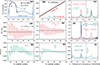 |
Fig. 2. (a): Brunt profile decomposed into a smooth part, N(u), and a glitch part, δN(u). (b): Pulsation periods vs radial order, k (l = 1 g modes). (c): Comparison between FT(ΔP) and the derivative of FT(δP/P). (d): Period spacings, ΔPk. (e): Relative period spacings, ΔPk, with respect to the asymptotic value, Πl. (f): Comparison of the Fourier spectrum of ΔPk and the buoyancy glitch derivatives. (g): Deviations (perturbations) of pulsation period from asymptotic values, δPk. (h): Relative perturbations of pulsation periods, δPk/Pk. (i): Comparison of the Fourier spectrum of δPk/Pk and the buoyancy glitch profile, δN/N. All plots are based on a middle-main-sequence (Xc = 0.4), M = 4.5 M⊙ stellar model, and its dipole g modes. |
It is important to note that we distinguish between δP, the deviation of the pulsation period from the linear, asymptotic relation (Pk ∝ k; Figure 2(b), and the observed period spacing, ΔPk = Pk + 1 − Pk (which is often used in the literature2). Figure 2(d) illustrates that ΔP oscillates around a mean value Πl. The normalized period spacing, (ΔPk − Πl)/Πl, is shown in Figure 2(e), which oscillates around zero on the order of ≈0.1. Similarly, the relative period perturbation, δP/P, is displayed in Figure 2(h). We note that δP/P is much smaller, only on the order of about ≲1%.
Figure 2(f) compares the one-sided Fourier amplitude spectrum FT(ΔPk − Πl)/Πl with the derivative of the Brunt glitch profile |dz(u)/dlnu|. This verifies Eq. (19). In practice, FT(ΔPk − Πl)/Πl is smoother due to its limited resolution.
Figure 2(i) highlights the comparison of FT(δP/P) and |z(u)| = |δN/N|. This validates Eq. (21). Again, the Fourier spectrum represents a “smoothed version” of the true glitch profile z(u).
Finally, the two Fourier spectra, FT(δP/P) and FT(ΔPk − Πl)/Πl, are directly linked by Eq. (22). The comparison of the red and green lines (respectively) in Figure 2(c) supports this relation. The Fourier spectra show symmetric super-Nyquist peaks; the peak at 0.7 appears to agree better with udFT(δP/P)/du than the actual peak at 0.3. This can be explained by a phase offset of 0.5 between u and ξ (see Sect. 3).
5. Effects of convective overshooting and mixing
We calculated stellar models with masses M = 1.6 M⊙ (representing a gDor star) and M = 3.2, 4.5, and 6.0 M⊙ (spanning roughly the SPB star mass range). We adopted convective-core overshooting parameters fov = 0.015, and 0.025, and the envelope mixing parameter Dmin = 10, 20, 50, and 100.
The right panel of Figure 3 shows the period-spacing varying frequency (uμ), i.e., the peak frequency of the normalized ΔPk Fourier spectra, as a function of the central hydrogen mass fraction, Xc, which serves as a proxy for main-sequence age. A strong, near-linear correlation is evident, with the best-fitting linear relation given by
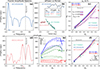 |
Fig. 3. Panel (b): Observed g-mode period spacings ΔP and periods for KIC 10526294, KIC 11145123, KIC 7760680. The Fourier spectra of KIC 10526294 and KIC 11145123 are shown in panel (a) and (d), respectively. The dominant peaks are labeled by the filled circles with the corresponding frequency, uμ. Panel (c) and (f): The g-mode ΔP variational frequency, uμ, is plotted as a function of central hydrogen mass fraction, Xc, for MESA models of masses M = 6.0 (blue), 3.2 (red) and 1.6 M⊙ (purple); (c) shows models with different convective-core overshooting, fov, and (f) displays the effect of the envelope mixing, Dmin. Panel (e) illustrates the amplitudes of FT(ΔP) for MESA models with different masses and Dmin. |
 (25)
(25)
Specifically, γ Dor models with M = 1.6 M⊙ all have uμ values below 0.5. For SPB stars, most main-sequence models with Xc ≳ 0.1 have uμ values below 0.5. However, for B-star models that are close to the Terminal Age Main Sequence (TAMS), the true peak in FT(ΔPk) can exceed 0.5, which reflects back to the sub-Nyquist region and produces a spurious peak symmetric to the real one.
Figures 1 and 3 (right column) can be compared with Miglio et al. (2008). In their Fig 15, they show an M = 1.6 M⊙γ Dor model, for which Xc = 0.5, 0.3, and 0.1 correspond to uμ = 0.09, 0.16, and 0.33, respectively. For the SPB star model with M = 6.0 M⊙ at the same Xc, the corresponding uμ values are larger: 0.15, 0.32, and 0.50 (their Fig 16).
For our calculations, the upper-right panel of Figure 3 shows that, at the same main-sequence age (Xc), models with larger overshooting result in higher values of uμ. This effect is more pronounced for the 1.6 M⊙ model than for the SPB star models. This agrees with the results of Miglio et al. (2008), who studied the effects of convective-core overshooting. For SPB stars, uμ, ov is only slightly larger than the non-overshooting counterpart uμ. However, for the gDor model, the difference is much more significant. As shown in Figs. 17 and 18 for the Xc = 0.3 model with αov = 0.2Hp, the difference in uμ is approximately 0.05.
Even with different levels of overshooting, the tight relation between uμ and Xc still holds, with a scatter of less than 0.1 in Xc. Similarly, the lower-right panel illustrates the effect of envelope mixing, Dmin. At the same Xc, a larger Dmin results in a slightly lower uμ, although the scatter is somewhat smaller than in the overshooting case.
Another observation is that, within the SPB star mass range, this tight correlation exhibits only a very weak dependence on stellar mass, indicating that uμ is a good age probe for any SPB stars regardless of their masses. For the γ Dor star model, the uμ − Xc curve lies well below the SPB-star fitting line.
We emphasize that even with different overshooting and mixing parameters, the tight relation between uμ and Xc still holds. The FT(ΔPk) peak frequency, uμ, can be used as an excellent age indicator for SPB stars, and remains a reliable age probe for γ Dor stars.
Miglio et al. (2008) also show that element diffusion smooths the Brunt profile, reducing local dN/du and lowering the peak in FT(ΔPk). Consequently, diffusion decreases the visibility of variations in ΔP (their Fig 21 and 22).
Based on MESA models with envelope mixing parameters Dmin = 10, 20, 50, and 100 and stellar masses M = 3.2, 4.5, and 6.0 M⊙, we measured the peak amplitude of the corresponding l = 1 g-mode period-spacing Fourier spectra and show the result in the lower-middle panel of Figure 3. As expected, the Brunt profile derivatives, and therefore the amplitude of FT(ΔP), depend sensitively on the mixing parameters, with larger Dmin resulting in significantly smaller amplitudes.
6. The effect of rotation on FT(ΔPk)
The derivations in Section 2 can be extended to rotating stars. Under the traditional approximation for rotation, the pulsation periods of gravity modes in the co-rotating frame can be described by
 (26)
(26)
We still have the variational relation for pulsation period perturbations,
![Mathematical equation: $$ \begin{aligned} \frac{\delta P_{k,co}}{P_{k,co}} \approx \int ^1_0{z\prime (u)[u-\cos (2\pi (k+k_0) u)/(2\pi (k+k_0))]\mathrm{d}u}. \end{aligned} $$](/articles/aa/full_html/2026/03/aa57374-25/aa57374-25-eq33.gif) (27)
(27)
Equation (7) can be rewritten as
 (28)
(28)
Following the analysis of Bouabid et al. (2013), the asymptotic co-rotating frame period spacing is given by
 (29)
(29)
where λl, m, s(k) is the eigenvalue of the Laplace tidal operator, which is generally a slowly varying function of k.
![Mathematical equation: $$ \begin{aligned}&\qquad \frac{\mathrm{d}\delta P_{k,co}}{\mathrm{d}k} \approx \frac{\Pi _0}{\sqrt{\lambda _{l,m,s(k)}}} \int ^1_0{z\prime (u)[u+u\sin (2\pi (k+k_0) u)]\mathrm{d}u}\nonumber \\&+\Pi _0 \int ^1_0{z\prime (u)[u(k+k_0)-\cos (2\pi (k+k_0) u)/(2\pi )]\mathrm{d}u}\frac{\mathrm{d}}{\mathrm{d}k}\left(\frac{1}{\sqrt{\lambda _{l,m,s(k)}}}\right). \end{aligned} $$](/articles/aa/full_html/2026/03/aa57374-25/aa57374-25-eq36.gif) (30)
(30)
We again ignore the second term using the slowly varying assumption of λ with respect to k.
Defining  , we obtain a similar result as Eq. (11),
![Mathematical equation: $$ \begin{aligned} \frac{\Delta P_{k,co,\mathrm{obs}}- \tilde{\Pi }_l }{\tilde{\Pi }_l} \approx \int ^1_0{z\prime (u)u [1 + \sin [2\pi (k+k_0) u]]\mathrm{d}u}. \end{aligned} $$](/articles/aa/full_html/2026/03/aa57374-25/aa57374-25-eq38.gif) (31)
(31)
To a good approximation, the Fourier spectra relations derived in Sect. 2 still hold, with the only difference being that the asymptotic period spacing, Πl, is replaced by  , and that we work in the co-rotating frame periods, Pk, co, and their spacings, ΔPk, co. We can therefore apply Equations (19) and (21) to observed g modes in rotating stars.
In practical applications, we transform the inertial (observer’s) frame periods, Pk, inert, to the co-rotating frame periods, Pk, co, using
 (32)
(32)
where we use the convention that m = −1, +1 corresponds to prograde and retrograde modes, respectively.
The corresponding period spacings are transformed as follows:
 (33)
(33)
 (34)
(34)
In the next section, we apply the above results to the g modes in the rotating SPB star KIC 7760680.
7. Applications to observations in g-mode pulsators
We applied the above results to the observed g modes in two slowly rotating stars, KIC 11145123 and KIC 10526294, where rotational effects on the g modes are negligible.
We then applied the rotation-corrected results in Section 6 to the rotating SPB star KIC 7760680.
7.1. Application to observations: Slowly rotating SPB and γ Dor stars
KIC 10526294 (B8V; ≈3.2 M⊙; Teff ≈ 11550K; log g ∼ 4.1; rotation period Prot ≈ 190 days) is an SPB pulsator that has been studied in detail by Pápics et al. (2014) and Moravveji et al. (2015). These authors identified the l = 1 prograde g modes, and their period-spacing pattern is shown in the upper-middle panel of Figure 3.
The upper-left panel of Figure 3 displays FT(ΔP), where the dominant peak occurs at uμ ≈ 0.059. Using Eq. (25), this value corresponds to Xc = 0.63 using Eq. (25), which agrees well with the detailed seismic modeling of Moravveji et al. (2015), who found Xc = 0.627. The peak amplitude of FT(ΔP) is 230.4 seconds and is also shown in the lower-middle panel of Figure 3.
KIC 11145123 (M ∼ 1.46 M⊙) also rotates very slowly, with an inferred rotation period of about 100 days (Kurtz et al. 2014). Its period-spacing agrees with a stellar model close to the TAMS, and the estimated Xc is as low as ≈0.033 although with large uncertainty. Our Fourier analysis of its period spacing reveals a peak at uμ ≈ 0.425 (Figure 3, lower-left panel), which is consistent with the low Xc result when compared with the 1.6 M⊙ model shown in the upper-right panel of Figure 3 (purple lines). A slightly lower mass (< 1.6 M⊙) appears more appropriate, similar to the value adopted by Kurtz et al. (2014). More detailed seismic modeling was carried out by Hatta et al. (2021), who find that non-standard modeling is required, supporting the argument that KIC 11145123 is likely a blue straggler.
For a typical 1.6 M⊙ model, the highest peaks of FT(ΔP) usually correspond to the sharply rising side of the Brunt profile (convective-core boundary), which occurs at very low u. The descending side of the Brunt profile is smoother than in SPB-star models and produces a broad, subdominant peak. Thus, in general, applying the FT(ΔP) technique to γ Dor stars is more challenging than applying it to SPB stars.
7.2. Application to the rotating SPB star KIC 7760680
KIC 7760680 is a rotating (frot ≈ 0.48day−1) SPB star. Pápics et al. (2015) identified 36 l = 1 prograde g modes from Kepler light curves. Spectroscopic observations placed the star at the low-mass end of the SPB instability strip. This agrees with the further seismic modeling by Moravveji et al. (2016), who derived the best-fitting model with a mass of M ≈ 3.25 and a central hydrogen fraction, Xc = 0.481.
The left two panels of Figure 4 show the observed l = 1, m = −1 (prograde) g-mode period spacings in both inertial frame (ΔPiner; green) and the co-rotating frame (ΔPco; blue). Transforming to the co-rotating frame removes the downward trend and makes the data ready for Fourier analysis. The Fourier spectrum of the normalized ΔPco versus k is shown in the upper-right panel. The dominant peak is at uμ ≈ 0.193, indicating a middle-main-sequence model with Xc ≈ 0.48. This value is in excellent agreement with the result of Moravveji et al. (2016). In fact, when placed on the uμ − Xc diagram, KIC 7760680 (green circle) lies directly on the fitting line shown in Figure 3 (right two panels).
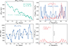 |
Fig. 4. Left column: Gravity-mode period spacing of KIC7760680 in the inertial frame (ΔPiner vs Piner, upper panel) and co-rotating frame (ΔPco vs Pco, lower panel). Right column: Fourier spectra of normalized ΔPco (upper) and the relative period perturbation, δPco/Pco (lower panel). The two spectra are linked by the relation |
![Mathematical equation: $ FT[(\Delta P -\tilde{\Pi}_l)/\tilde{\Pi}_l]=\mathrm{d}FT(\delta P/P)/\mathrm{d}\ln u $](/articles/aa/full_html/2026/03/aa57374-25/aa57374-25-eq43.gif)
The Fourier spectrum of the relative period perturbation, δPco/Pco, is shown in the lower-right panel of Figure 4. It indicates that a relative buoyancy glitch, δN/N, of the order 0.2%, located at three distinct regions responsible for the periodic variations in the g-mode period spacings. We calculated the derivative of the spectrum, dFT(δPco/Pco)/dlnu, and plot it in the upper-left panel (red line). According to Eq. (22), this is directly equal to the Fourier spectrum of the period spacing FT(ΔPk) (up to a 0.5 phase offset in practice). The red line follows the blue curve reasonably well, further supporting our theoretical results.
We do not include the FT(ΔP) amplitude measurement of KIC 7760680 in the lower-middle plot of Figure 3, because the ΔP amplitude depends on the reference frame and the rotation rate (as illustrated in the left column of Figure 4).
8. Discussion and conclusions
8.1. Ensemble asteroseismology of g-mode pulsators with FT(ΔP)
Because this method is straightforward, it facilitates the ensemble seismology of g-mode pulsators. About 611 γ Dor stars were analyzed in Li et al. (2019, 2020), and a significant fraction show period-spacing variations. Pedersen et al. (2018, 2021) performed detailed seismic modeling on26 SPB stars By analyzing the measured FT(ΔP) frequencies and their amplitudes, we can identify correlations among stellar age, convective overshooting, mixing parameters, rotation, and other related factors.
Since the Fourier spectra of period spacings and period perturbations depend only on the Brunt glitch profile z(u) and its derivatives, there is essentially no l-dependence. Consequently, ΔP for different l should display the same variation period. We have already confirmed this in observations and will present the results in a separate paper. In fact, by including both l = 1 and l = 2 modes, we double the number of data points, which improves the resolution of the Fourier spectra and thus further constrains the main-sequence age, Xc, and the mixing and overshooting parameters.
8.2. Other g-mode pulsators: Compact pulsators, He-burning red giants, and beyond
This technique can also be applied to other pulsators that exhibit g modes. Compact pulsators such as sdB stars and white dwarfs have several different chemical gradient layers or interfaces. Gravity modes can also be trapped in these layers (Brassard et al. 1992), leading to deep dips in the period spacings. By connecting eigenfunctions and using continuity conditions, Charpinet et al. (2000) derived analytical expressions for the period spacing between consecutive trapped modes and related them to the H-He transition layers. It remains to be seen whether the FT(ΔP) technique can be applied to these pulsators that exhibit very deep period-spacing dips.
The related He-core-burning red giants also contain multiple chemical gradient layers. Bossini et al. (2015) showed that the He-burning shell at u ≈ 0.7, as a glitch, is too smooth to give rise to significant deviations from the asymptotic period spacings. However, another glitch at u ≈ 0.17, caused by a discontinuity in local opacity, induces a periodicity of Δk ≈ 6 in the g-mode period spacings. Matteuzzi et al. (2025) investigated the influence of density-discontinuity-induced buoyancy structural glitches on the period spacings of these oscillation modes in these stars.
As shown in Figure 4, KIC 7760680 exhibits additional peaks in FT(ΔP) at u ≈ 0.02. This may correspond to the low-frequency subdominant peak near u = 0, as illustrated in Figure 1. Detecting multiple periods in ΔP for more g-mode pulsators is therefore very promising.
We also verified the FT(ΔP) technique for post-mass transfer stellar models (Wagg et al. 2024; Henneco et al. 2024; Miszuda et al. 2025). These models may have subtle differences in the Brunt profile due to mass accretion, and the additional periodic signal can be detected directly from the period spacing variations (Wu et al. 2026).
8.3. Comparison with classical structure inversions
This technique provides an efficient way to reconstruct the Brunt glitch profile z(u), which can be cross-checked with classical stellar structure inversion techniques such as Optimally Localized Averages (OLA) and Regularized Least Squares (RLS). Moreover, Vanlaer et al. (2023) explored the applications of these inversions to both the Brunt profile and density-sound-speed pairs.
8.4. Linking g-mode asteroseismology to tidal evolution studies
Remarkably, the key Brunt glitch profile derivative  is extremely similar to the term
  that appears in the tidal torque expression and is directly linked to the timescale of tidal evolution and dissipation and E2. Its value at the convective-radiative boundary appears in the tidal torque expression, which crucially determines the tidal evolution and dissipation timescale associated with E2 (Zahn 1970, 1975; Barker 2020). Indeed, internal gravity waves (IGWs) are generated at the convective-radiative boundary and propagate outward in intermediate- and massive stars, or inward in low-mass stars such as the Sun. The tidal Love number klm, particularly k2, also depends on this derivative, which is key to the apsidal motion of binary stars. Linking the observed g-mode period spacings to the derivative of the Brunt profile (glitches) opens an avenue to connect gravity-mode asteroseismology to tidal evolution studies.
8.5. Limitations of the FT(ΔP) technique
This method is applicable only to g modes that exhibit clear period-spacing variations and ideally a larger number of modes. We applied this technique to the g modes of SPB stars analyzed by Pedersen et al. (2018) (Guo & Aerts 2025), which exhibit a number of detected g modes ranging from N = 6 to N = 23. We find that the FT(ΔP) technique remains effective even for stars with a very limited number of g modes (as few as N = 6). However, misidentification or incompleteness of the ΔP series can significantly affect the results if the range of observed periods is not well covered. It should also be noted that with a limited number of modes, the classical approach of assigning error bars to frequencies in the Fourier spectrum based on the signal-to-noise ratio is no longer valid. Instead, a Monte Carlo or bootstrapping method should be employed to estimate the uncertainties.
Since we rely on the variational result to link pulsation perturbation to the Brunt profile perturbation, the theoretical relations in Sect. 2 and 5 apply only to g modes with small relative period perturbations, δP/P. This is usually the case for SPB and γ Dor stars, but may not hold for sdB and white dwarfs, which feature multiple chemical transition regions with sharper Brunt profile gradients. For large-amplitude glitches, we can decompose the glitch into a series of small-amplitude glitches and apply the FT(ΔP) technique to each (Zhang et al. 2023). However, this increases complexity, for example, by introducing harmonic peaks. We can mitigate these by using the pre-whitening or CLEAN algorithms to remove spurious peaks. This approach remains a promising tool for probing the chemical composition gradients in stellar interiors.
|The analysis uses only the first-order asymptotic period relation in Eq. (3), which ignores the second- and higher-order terms. We have also not fully exploited the information on the amplitudes of FT(ΔP), i.e., Brunt profile derivatives from models. Constructing denser grids of stellar models with varying mixing and overshooting parameters can further constrain the desired stellar parameters. Additionally, we did not consider rotating stellar models. A large number of FT(ΔP) amplitude measurements could potentially constrain rotational mixing in stellar structure computations and different convective-mixing schemes (Noll et al. 2024).
Pulsational period spacings of γ Dor stars sometimes exhibit dips that are induced by coupling between the pure inertial mode in the convective and gravity modes (Saio et al. 2021; Ouazzani et al. 2020). Our technique is not adequate for modeling these variations (dips) in period spacings.
8.6. Core-envelope symmetry
Montgomery et al. (2003) showed that a buoyancy glitch δN/N and its reflected version around u = 0.5 induced the same g-mode period perturbations. They referred to this as the inherent core-envelope symmetry, which can lead to ambiguity in determining the location of features such as composition transition zones. As shown earlier, this symmetry is a natural consequence of the normalized buoyancy radius u being equivalent to the frequency ξ and the symmetry around the Nyquist frequency at 0.5.
We summarize the procedures for analyzing observed g-mode periods Pk, obs that exhibit small dips as follows: 1. Identify the spherical degree, l, and azimuthal order, m. Fit the asymptotic relation,  to determine the asymptotic period spacing, Π0, and rotational frequency, frot. This step can be performed using the AMIGO package (Van Reeth et al. 2016). 2. Convert the pulsation periods and period spacings to the co-rotating frame and then compute the deviations of the pulsation periods from the asymptotic relation, δP. 3. Perform a Fourier transform of normalized ΔPk and δP/P as a function of the radial order, k (the exact values of k are critical). 4. Identify the peak frequency, uμ, and its amplitude in the Fourier spectra, FT(ΔPk). For stars near the terminal-age main sequence (TAMS), exercise caution when selecting the correct peak (uμ can exceed 0.5) and avoid spurious reflection peaks.
Acknowledgments
We thank Conny Aerts, Tao Wu, Joel Ong and Gang Li for helpful discussions. The research leading to these results has received funding from the European Research Council (ERC) under the Horizon Europe programme (Synergy Grant agreement N°101071505: 4D-STAR). While funded by the European Union, views and opinions expressed are however those of the author(s) only and do not necessarily reflect those of the European Union or the European Research Council. Neither the European Union nor the granting authority can be held responsible for them.
References
- Althaus, L. G., Córsico, A. H., Isern, J., & García-Berro, E. 2010, A&ARv, 18, 471 [NASA ADS] [CrossRef] [Google Scholar]
- Barker, A. J. 2020, MNRAS, 498, 2270 [Google Scholar]
- Basu, S. 1997, MNRAS, 288, 572 [NASA ADS] [Google Scholar]
- Bossini, D., Miglio, A., Salaris, M., et al. 2015, MNRAS, 453, 2290 [Google Scholar]
- Bouabid, M. P., Dupret, M. A., Salmon, S., et al. 2013, MNRAS, 429, 2500 [Google Scholar]
- Brassard, P., Fontaine, G., Wesemael, F., & Hansen, C. J. 1992, ApJS, 80, 369 [NASA ADS] [CrossRef] [Google Scholar]
- Charpinet, S., Fontaine, G., Brassard, P., & Dorman, B. 2000, ApJS, 131, 223 [Google Scholar]
- Christensen-Dalsgaard, J. 1988, IAU Symp., 123, 295 [Google Scholar]
- Córsico, A. H., Althaus, L. G., Miller Bertolami, M. M., & Kepler, S. O. 2019, A&ARv, 27, 7 [Google Scholar]
- Cunha, M. S., Avelino, P. P., Christensen-Dalsgaard, J., et al. 2019, MNRAS, 490, 909 [Google Scholar]
- Cunha, M. S., Damasceno, Y. C., Amaral, J., et al. 2024, A&A, 687, A100 [NASA ADS] [CrossRef] [EDP Sciences] [Google Scholar]
- Degroote, P., Aerts, C., Baglin, A., et al. 2010, Nature, 464, 259 [Google Scholar]
- Guo, Z., & Aerts, C. 2025, ArXiv e-prints [arXiv:2512.08155] [Google Scholar]
- Guyot, N., Van Grootel, V., Charpinet, S., et al. 2025, A&A, 696, A13 [NASA ADS] [CrossRef] [EDP Sciences] [Google Scholar]
- Hatta, Y. 2023, ApJ, 950, 165 [NASA ADS] [CrossRef] [Google Scholar]
- Hatta, Y., Sekii, T., Takata, M., & Benomar, O. 2021, ApJ, 923, 244 [NASA ADS] [CrossRef] [Google Scholar]
- Henneco, J., Van Reeth, T., Prat, V., et al. 2021, A&A, 648, A97 [EDP Sciences] [Google Scholar]
- Henneco, J., Schneider, F. R. N., Hekker, S., & Aerts, C. 2024, A&A, 690, A65 [NASA ADS] [CrossRef] [EDP Sciences] [Google Scholar]
- Herwig, F. 2000, A&A, 360, 952 [NASA ADS] [Google Scholar]
- Kurtz, D. W., Saio, H., Takata, M., et al. 2014, MNRAS, 444, 102 [Google Scholar]
- Li, G., Bedding, T. R., Murphy, S. J., et al. 2019, MNRAS, 482, 1757 [Google Scholar]
- Li, G., Van Reeth, T., Bedding, T. R., et al. 2020, MNRAS, 491, 3586 [Google Scholar]
- Lignières, F., Ballot, J., Deheuvels, S., & Galoy, M. 2024, A&A, 683, A2 [NASA ADS] [CrossRef] [EDP Sciences] [Google Scholar]
- Matteuzzi, M., Buldgen, G., Dupret, M.-A., et al. 2025, A&A, 700, A261 [NASA ADS] [CrossRef] [EDP Sciences] [Google Scholar]
- Miglio, A., Montalbán, J., Noels, A., & Eggenberger, P. 2008, MNRAS, 386, 1487 [Google Scholar]
- Miszuda, A., Guo, Z., & Townsend, R. H. D. 2025, A&A, 702, A203 [NASA ADS] [CrossRef] [EDP Sciences] [Google Scholar]
- Montgomery, M. H., Metcalfe, T. S., & Winget, D. E. 2003, MNRAS, 344, 657 [NASA ADS] [CrossRef] [Google Scholar]
- Moravveji, E., Aerts, C., Pápics, P. I., Triana, S. A., & Vandoren, B. 2015, A&A, 580, A27 [NASA ADS] [CrossRef] [EDP Sciences] [Google Scholar]
- Moravveji, E., Townsend, R. H. D., Aerts, C., & Mathis, S. 2016, ApJ, 823, 130 [NASA ADS] [CrossRef] [Google Scholar]
- Mosser, B., Benomar, O., Belkacem, K., et al. 2014, A&A, 572, L5 [NASA ADS] [CrossRef] [EDP Sciences] [Google Scholar]
- Noll, A., Basu, S., & Hekker, S. 2024, A&A, 683, A189 [NASA ADS] [CrossRef] [EDP Sciences] [Google Scholar]
- Ong, J. M. J., Basu, S., & Roxburgh, I. W. 2021, ApJ, 920, 8 [NASA ADS] [CrossRef] [Google Scholar]
- Ouazzani, R. M., Lignières, F., Dupret, M. A., et al. 2020, A&A, 640, A49 [NASA ADS] [CrossRef] [EDP Sciences] [Google Scholar]
- Pápics, P. I., Moravveji, E., Aerts, C., et al. 2014, A&A, 570, A8 [NASA ADS] [CrossRef] [EDP Sciences] [Google Scholar]
- Pápics, P. I., Tkachenko, A., Aerts, C., et al. 2015, ApJ, 803, L25 [Google Scholar]
- Paxton, B., Bildsten, L., Dotter, A., et al. 2011, ApJS, 192, 3 [Google Scholar]
- Paxton, B., Cantiello, M., Arras, P., et al. 2013, ApJS, 208, 4 [Google Scholar]
- Pedersen, M. G., Aerts, C., Pápics, P. I., & Rogers, T. M. 2018, A&A, 614, A128 [NASA ADS] [CrossRef] [EDP Sciences] [Google Scholar]
- Pedersen, M. G., Aerts, C., Pápics, P. I., et al. 2021, Nat. Astron., 5, 715 [NASA ADS] [CrossRef] [Google Scholar]
- Roxburgh, I. W., & Vorontsov, S. V. 1994, MNRAS, 268, 880 [NASA ADS] [CrossRef] [Google Scholar]
- Rui, N. Z., Ong, J. M. J., & Mathis, S. 2024, MNRAS, 527, 6346 [Google Scholar]
- Saio, H., Takata, M., Lee, U., Li, G., & Van Reeth, T. 2021, MNRAS, 502, 5856 [Google Scholar]
- Shi, X.-D., Qian, S.-B., Zhu, L.-Y., & Li, L.-J. 2023, ApJS, 268, 16 [CrossRef] [Google Scholar]
- Sun, M., Townsend, R. H. D., & Guo, Z. 2023, ApJ, 945, 43 [NASA ADS] [CrossRef] [Google Scholar]
- Sutherland, B. R. 2010, Internal Gravity Waves (Cambridge University Press), 394 [Google Scholar]
- Szewczuk, W., & Daszyńska-Daszkiewicz, J. 2018, MNRAS, 478, 2243 [Google Scholar]
- Tassoul, M. 1980, ApJS, 43, 469 [Google Scholar]
- Townsend, R. H. D., & Teitler, S. A. 2013, MNRAS, 435, 3406 [Google Scholar]
- Townsend, R. H. D., Goldstein, J., & Zweibel, E. G. 2018, MNRAS, 475, 879 [Google Scholar]
- Turner, J. S. 1973, Buoyancy Effects in Fluids (Cambridge University Press), 368 [Google Scholar]
- Uzundag, M., Baran, A. S., Østensen, R. H., et al. 2017, MNRAS, 472, 700 [CrossRef] [Google Scholar]
- Van Reeth, T., Tkachenko, A., & Aerts, C. 2016, A&A, 593, A120 [NASA ADS] [CrossRef] [EDP Sciences] [Google Scholar]
- Vanlaer, V., Aerts, C., Bellinger, E. P., & Christensen-Dalsgaard, J. 2023, A&A, 675, A17 [NASA ADS] [CrossRef] [EDP Sciences] [Google Scholar]
- Wagg, T., Johnston, C., Bellinger, E. P., et al. 2024, A&A, 687, A222 [NASA ADS] [CrossRef] [EDP Sciences] [Google Scholar]
- Wu, T., Li, Y., & Deng, Z.-M. 2018, ApJ, 867, 47 [NASA ADS] [CrossRef] [Google Scholar]
- Wu, T., Li, Y., Deng, Z.-M., et al. 2020, ApJ, 899, 38 [NASA ADS] [CrossRef] [Google Scholar]
- Wu, T., Guo, Z., & Li, Y. 2026, A&A, 705, A164 [NASA ADS] [CrossRef] [EDP Sciences] [Google Scholar]
- Zahn, J. P. 1970, A&A, 4, 452 [NASA ADS] [Google Scholar]
- Zahn, J. P. 1975, A&A, 41, 329 [NASA ADS] [Google Scholar]
- Zhang, Q.-S., Li, Y., Wu, T., & Jiang, C. 2023, ApJ, 953, 9 [NASA ADS] [CrossRef] [Google Scholar]
We are not interested in the near-surface region, where N can be large.
Some literature uses δP to denote the period spacing.
All Figures
|
Fig. 1. Brunt–Väisälä (buoyancy) profiles, period spacings and their Fourier spectra for an M = 3.2 M⊙ MESA stellar model. Profiles are plotted as a function of the radial coordinate x = r/R (left panels) and the buoyancy coordinate, u (middle panels), with solar metallicity and convective overshooting, fov = 0.015. The hydrogen mass fraction, X, is shown by dashed green lines (multiplied by 10 for clarity). The gray-shaded regions denote the receding convective core. The dipole gravity-mode period spacings, ΔPk, are shown in the right panels, and their Fourier amplitude spectra, FT(ΔP), are overplotted in the middle panels (red lines, with super-Nyquist components in gray). The dominant Fourier-spectrum peak aligns with the sharp drop points of the Brunt profile and is labeled as uμ in red. |
| In the text | |
|
Fig. 2. (a): Brunt profile decomposed into a smooth part, N(u), and a glitch part, δN(u). (b): Pulsation periods vs radial order, k (l = 1 g modes). (c): Comparison between FT(ΔP) and the derivative of FT(δP/P). (d): Period spacings, ΔPk. (e): Relative period spacings, ΔPk, with respect to the asymptotic value, Πl. (f): Comparison of the Fourier spectrum of ΔPk and the buoyancy glitch derivatives. (g): Deviations (perturbations) of pulsation period from asymptotic values, δPk. (h): Relative perturbations of pulsation periods, δPk/Pk. (i): Comparison of the Fourier spectrum of δPk/Pk and the buoyancy glitch profile, δN/N. All plots are based on a middle-main-sequence (Xc = 0.4), M = 4.5 M⊙ stellar model, and its dipole g modes. |
| In the text | |
|
Fig. 3. Panel (b): Observed g-mode period spacings ΔP and periods for KIC 10526294, KIC 11145123, KIC 7760680. The Fourier spectra of KIC 10526294 and KIC 11145123 are shown in panel (a) and (d), respectively. The dominant peaks are labeled by the filled circles with the corresponding frequency, uμ. Panel (c) and (f): The g-mode ΔP variational frequency, uμ, is plotted as a function of central hydrogen mass fraction, Xc, for MESA models of masses M = 6.0 (blue), 3.2 (red) and 1.6 M⊙ (purple); (c) shows models with different convective-core overshooting, fov, and (f) displays the effect of the envelope mixing, Dmin. Panel (e) illustrates the amplitudes of FT(ΔP) for MESA models with different masses and Dmin. |
| In the text | |
|
Fig. 4. Left column: Gravity-mode period spacing of KIC7760680 in the inertial frame (ΔPiner vs Piner, upper panel) and co-rotating frame (ΔPco vs Pco, lower panel). Right column: Fourier spectra of normalized ΔPco (upper) and the relative period perturbation, δPco/Pco (lower panel). The two spectra are linked by the relation |
| In the text | |
Current usage metrics show cumulative count of Article Views (full-text article views including HTML views, PDF and ePub downloads, according to the available data) and Abstracts Views on Vision4Press platform.
Data correspond to usage on the plateform after 2015. The current usage metrics is available 48-96 hours after online publication and is updated daily on week days.
Initial download of the metrics may take a while.