| Issue |
A&A
Volume 707, March 2026
|
|
|---|---|---|
| Article Number | A224 | |
| Number of page(s) | 27 | |
| Section | Planets, planetary systems, and small bodies | |
| DOI | https://doi.org/10.1051/0004-6361/202557439 | |
| Published online | 23 March 2026 | |
A consistent numerical integration of orbit, tides, and rotation for synchronous satellites
1
European Space Agency (ESA), European Space Research and Technology Centre (ESTEC),
Keplerlaan 1,
2201 AZ
Noordwijk,
The Netherlands
2
Delft University of Technology,
Kluyverweg 1,
2629 HS
Delft,
The Netherlands
★ Corresponding author: This email address is being protected from spambots. You need JavaScript enabled to view it.
Received:
26
September
2025
Accepted:
19
December
2025
Abstract
Context. Consistently modelling the effects of the tides raised on a satellite on the dynamics of the satellite itself and on those of a nearby spacecraft (either in orbit or performing a flyby) requires accounting for the instantaneous tidal deformation of the satellite’s gravitational potential. For synchronous satellites, the spin-orbit resonance causes perfect commensurability between the orbital and rotational periods, and the main tidal forcing frequency. This imposes stringent consistency requirements on the modelling of the delicate interplay between the satellite’s orbital motion, rotational dynamics, and tidal deformation. These three aspects of satellite dynamics are typically handled separately (at least partially) in classical modelling approaches, which are therefore highly inconsistency-prone for the specific spin-orbit resonance case.
Aims. Modelling inconsistencies can lead to the under- or overestimation of tidal parameters when dissipation signatures are extracted simultaneously from both spacecraft and moon dynamics, a combined approach that is increasingly critical for current and upcoming mission analyses. As a promising alternative, we propose a coupled integration of the satellite’s orbit, rotation, and tidal deformation.
Methods. Integrating the satellite’s deformation requires introducing an additional set of differential equations for its degree-two gravity coefficients to complement the translational and rotational equations of motion. A concurrent integration ensures that the satellite’s instantaneous tidal response is fully consistent with its orbit and rotation, while automatically accounting for all dynamical couplings at play. In this paper, we present a two-dimensional implementation of this coupled propagation framework and investigate its ability to produce realistic dynamics with expected tidal dissipation signatures. As a proof-of-concept, we validated the physical self-consistency of the results using the Earth–Moon and Mars–Phobos systems as conceptual test cases.
Results. Our coupled propagation naturally maintains the spin-orbit resonance while producing the expected orbital migration and circularisation rates (including libration-induced tidal dissipation enhancement in the case of Phobos), a delicate balance that is hard to achieve with decoupled modelling strategies. The time history of the satellite’s gravitational tidal response (obtained as a direct output of our integration) is also in agreement with analytical predictions derived from the tidal potential theory.
Conclusions. Our coupled approach thus provides a unified and consistent way to model orbit-rotation-tide interactions. Crucially, it is equally applicable to representing tidal effects on the satellite itself and on a nearby spacecraft. This is critical for planetary missions such as Juice and Europa Clipper, where tidal dissipation signatures can (and will) be extracted from both the spacecraft’s and moons’ dynamics.
Key words: methods: numerical / celestial mechanics / planets and satellites: general
© The Authors 2026
 Open Access article, published by EDP Sciences, under the terms of the Creative Commons Attribution License (https://creativecommons.org/licenses/by/4.0), which permits unrestricted use, distribution, and reproduction in any medium, provided the original work is properly cited.
This article is published in open access under the Subscribe to Open model. This email address is being protected from spambots. You need JavaScript enabled to view it. to support open access publication.
1 Introduction
Tides, both those raised on the central planet and those on natural satellites, are key drivers of the long-term evolution of planetary systems. The amount of energy dissipated due to satellite tides1 governs the tidal heating rate of the moons’ interiors, and therefore plays a crucial role in their thermal evolution (e.g., Peale & Cassen 1978; Peale et al. 1979). Additionally, the combined effects of satellite and planet tides define the moons’ orbital migration and circularisation rates (e.g., Kaula 1964; Goldreich & Soter 1966), and influence the system’s rotational dynamics (e.g., Goldreich & Gold 1963; MacDonald 1964; Efroimsky & Williams 2009). The present orbit, rotational state, and interior properties of the satellite, on the other hand, determine how much energy is currently dissipated due to tides (see Tobie et al. 2025, and references therein). The system’s dynamical and interior evolution is therefore driven by this intricate feedback between the moons’ orbit, rotation, and tidal response.
Reconstructing the orbits of natural satellites, for instance in ephemeris determination studies, thus requires accounting for the effects of tides on the moons’ dynamics, but also provides us with a natural way to quantify tidal dissipation, both within the central planet or its synchronous satellite(s). Our present knowledge of tidal dissipation parameters beyond the Earth–Moon system primarily comes from astrometry-based constraints on the secular evolution of the moons’ orbits (e.g., Lainey et al. 2009; Lainey 2016; Lainey et al. 2020; Jacobson 2022). From a dynamical modelling perspective, these studies, which investigate long timescales compared to the satellite’s orbital period, only require the averaged long-term effects of planet and satellite tides to be accurately accounted for. Critically, this does not necessitate directly modelling the tidal deformation of the satellite’s gravity field, nor the instantaneous tidal effects on the system’s dynamics. A separate tidal acceleration added to the satellite’s equations of motion is instead sufficient to capture the long-term signature of tidal dissipation in the moons’ dynamics (e.g., Lainey et al. 2007; Lari 2018, see Section 3.4), and therefore perfectly suitable for the determination of ephemerides and dissipation parameters based on direct observations of the moons’ orbits.
However, incorporating tracking data from planetary missions into such ephemeris estimations requires a shift in our modelling paradigm. Spacecraft tracking data are sensitive to tidal signatures both in the spacecraft’s and in the moons’ dynamics (e.g., Magnanini et al. 2024; Fayolle 2025). Whenever in orbit or performing a flyby, the spacecraft’s trajectory is affected by the gravitational response of the tidally deforming moon, but is also influenced by the moon’s own orbit around the central planet, and therefore by tidal effects present in the moon’s dynamics. Accounting for the combined signatures of these different tidal effects in the spacecraft data in a fully consistent manner, critical for a robust estimation of tidal parameters, ideally requires using a single unified model (Fayolle et al. 2022).
However, as mentioned above, tidal effects on the moons’ orbits are typically modelled as an additional perturbing acceleration based on the averaged effect of tides, circumventing the need to model the time-varying tidal deformation of the moon’s gravitational potential. Nonetheless, explicit modelling of the latter becomes necessary to incorporate tides in the spacecraft’s dynamics. In practice, this is typically achieved by introducing gravity coefficient variations, which are defined by the moon’s instantaneous state and orientation (Petit et al. 2010; Iess et al. 2012; Goossens et al. 2024; Park et al. 2025). In principle, directly accounting for satellite tides in the moon’s (time-varying) gravity field in such a way also allows us to model their feedback on the moon’s own dynamics, thus offering a single, coherent way to encapsulate both effects. However, unique challenges arise when attempting to consistently model the impact on the orbital dynamics of the deformation of a synchronous satellite’s gravity field due to tides, and most critically the effects of such gravitational deformation on the satellite’s own orbit and rotation (Fayolle 2025).
In particular, the uniqueness of the challenges arising in the spin-orbit resonance case stems from the leading tidal forcing modes becoming commensurable with the orbital and rotational frequencies (and its harmonics) (e.g., Efroimsky & Williams 2009; Efroimsky 2012). This implies stringent consistency requirements for the satellite’s orbit, rotation, and gravity field tidal deformation, to ensure that this commensurability is maintained at the required accuracy level. Even a small inconsistency in the delicate interplay between translational and rotational dynamics when modelling synchronous satellite tides would indeed lead to unphysical dynamics, either breaking the spin-orbit resonance or mis-estimating the moon’s orbital migration rate (see Magnanini et al. 2026).
Starting from Kaula’s tidal potential expansion (Kaula 1964), numerous past analytical studies have provided a thorough characterisation of satellite tides, including (among others) a theoretical quantification of the amount of energy they dissipate (e.g., Efroimsky & Makarov 2014; Frouard & Efroimsky 2017; Efroimsky 2018), and of their effects on the moon’s orbit (Boué & Efroimsky 2019) and rotation (Efroimsky & Williams 2009; Efroimsky 2012; Williams & Efroimsky 2012; Makarov & Efroimsky 2013). These analytical developments provide us with invaluable insights into the expected manifestations, effects, and signatures of satellite tides. They, however, cannot be directly incorporated in dynamical models of synchronous satellites when fitting real ground-based and/or space-based data. When propagating the moon’s translational dynamics (as required in ephemeris studies and tidal parameter estimation analyses), the exact tidal forcings are no longer known a priori. They are instead influenced by the satellite’s integrated orbit, and are thus an outcome of the numerical propagation. The orbit-rotation-tides interplay then becomes sensitive to the satellite’s (numerically integrated) dynamical response to instantaneous perturbations and, most critically, to any inconsistency in the modelling of that response. This directly conflicts with the strict orbit-rotation-tidal response consistency requirement discussed above for the spin-orbit resonance case. What is required to meet the needs presented by (future) Earth- and space-based tracking data is a model for the tidal gravity field variation of a synchronously rotating satellite that can automatically and consistently adapt itself to variations in orbit and rotation during a numerical propagation of the dynamics.
To address the aforementioned challenges when modelling the gravitational deformation of a synchronous satellite undergoing tidal forcing, we therefore propose a coupled, concurrent propagation of the satellite’s orbit, rotation, and gravity field deformation. This approach follows the framework adopted, for instance, in Correia et al. (2014) and Boué et al. (2016) to study exo-planetary systems. The tidal deformation of the satellite’s gravity field, represented by its spherical harmonics coefficients, is described by an ordinary differential equation and numerically integrated alongside the translational and rotational equations of motion. Such a unified modelling approach automatically accounts for all dynamical couplings and feedbacks at play, while ensuring that the tidally induced gravity deformation remains consistent with the satellite’s orbit, rotation, and assumed rheology, at any instant of the propagation.
As mentioned above, ensuring the consistency between the orbit, tides, and rotation is extremely challenging with classical approaches where they are typically modelled separately, in a decoupled manner. With our coupled model, on the other hand, the self-consistency between the orbital, rotational, and tidal dynamics is naturally maintained throughout the propagation. The ability of our model to produce realistic dynamics, however, becomes contingent upon the determination of a suitable and consistent initial state (to be addressed in Section 5.2). This is a critical challenge when adopting such a coupled modelling strategy: any inconsistency upon initialisation would affect the orbit-rotation-tide interplay and result in a self-consistent yet physically unrealistic solution.
Our paper describes this extended coupled dynamical model and its implementation in a simplified two-dimensional case. As a conceptual validation to motivate further developments for ephemerides applications, we used this simplified propagation test case to show the applicability of such a coupled approach for planet – synchronous satellite systems. In particular, this paper demonstrates our model’s self-consistent representation of the tides-orbit-rotation interplay, while discussing the limitations of currently typical decoupled approaches for the particular case of tides in synchronous satellites. To this end, we leveraged insights from the tidal potential theory to justify the need for our coupled approach, and provided an analytical framework against which to compare our results. We emphasise that the present work presents a proof-of-concept implementation of this unified, fully consistent propagation, which can be used to scrutinise its behaviour and assess its suitability, but is not yet applicable to real data fitting.
Classical models (i.e., tidal effects incorporated as a perturbing acceleration for the moon’s dynamics or as time variations of the moon’s gravity field for the spacecraft’s dynamics) are perfectly suitable when separately considering tidal signatures either in the moon’s or in the spacecraft’s orbit, respectively. Typical natural satellite ephemerides applications (e.g., Lainey et al. 2009, 2012, 2020) and geodetic parameter estimations (e.g., Williams et al. 2014; Lemoine et al. 2013; Durante et al. 2019; Park et al. 2025) are therefore largely unaffected by the modelling complications outlined above. The latter only arise when concurrently modelling and/or extracting the combined tidal signatures in the two types of dynamics, and only for a synchronous satellite.
However, this concurrent modelling of tidal effects (and the associated challenges mentioned above) has become essential for current and upcoming analyses, given the unprecedented size, diversity, and quality of the available datasets. For the upcoming Juice (Jupiter Icy Moons Explorer) (Grasset et al. 2013; Van Hoolst et al. 2024) and Europa Clipper (Pappalardo et al. 2024) missions, tidal dissipation signatures in the moons’ own dynamics and in the spacecraft’s orbit are expected to be both detectable from the spacecraft tracking data, given the expected accuracy level. Even in cases where the dissipation occurring within the moon is too weak for its effect to be visible in spacecraft tracking data, the unified propagation model proposed in this work can still be desirable. By naturally accounting for all dynamical inter-dependencies, such a model prevents moon ephemeris and spacecraft orbit determination errors from affecting estimates of geodetic or rotation parameters. Decoupled analysis of past missions such as Cassini (Durante et al. 2019) have identified possible inconsistencies between orbit, rotation, and gravity solutions (including tidal response) as potential sources of error or discrepancy. Adopting a fully coupled and consistent dynamical model, on the contrary, would facilitate physically realistic and statistically robust estimation solutions. In addition to Juice and Europa Clipper, other current and upcoming missions such as MMX (Martian Moons eXploration) or Hera, but also future icy moon missions (NASA’s Uranus Orbiter and Probe (UOP) or ESA’s L4 concept mission to Enceladus) could benefit from the coupled propagation framework proposed here.
Progressively building the complete analytical framework necessary for the set-up and interpretation of our coupled dynamical model, we start by briefly describing the translational and rotational dynamics in Section 2. Section 3 then describes tides in a planet – synchronous satellite system, including an overview of relevant aspects of tidal theory, expected tidal effects on the satellite’s orbit and rotation, as well as existing modelling strategies and their potential limitations. Section 4 proposes a different tidal modelling strategy and introduces the deformation model used to numerically propagate the gravity coefficient variations. Section 5 then summarises the complete formulation of our coupled orbital-rotational-tidal model and describes the propagation set-ups for both the Earth–Moon and Mars–Phobos systems, which we use as test cases for our model. We concurrently propagated the satellite’s orbital dynamics, rotational motion, and tidal deformation in both systems to verify the behaviour of our coupled model, and its modelling of tidal dissipation effects in particular. In Section 6, we present the results of these coupled propagations and we investigate them in Section 7 in light of relevant insights from the tidal theory outlined in Section 3. Finally, the conclusions, implications, and foreseen future developments are discussed in Section 8.
2 Translational-rotational dynamics
As a necessary background for the tidal theory presented in Section 3 and its application in the present context, we first provide an overview of the well-known equations of motion governing the translational and rotational dynamics of a planet–satellite system. We restrict our models to the gravitational interactions between the planet and satellite. Since our work focusses on modelling the effects of satellite tides on the system’s dynamics, perturbations due to third-body interactions and non-conservative forces are not considered here.
2.1 Translational dynamics
Following Lainey et al. (2004), the inertial (i.e., non-rotating frame origin) acceleration of body i with respect to body j due to its gravitational interaction with j, noted  , can be decomposed into point mass and extended body interactions:
 (1)
(1)
where  and
and  respectively designate the point mass and extended body components of the gravitational potential of body k. The final term corresponds to figure-figure interactions, and can typically be safely neglected in planet–satellite dynamics (e.g., Lainey et al. 2004; Dirkx et al. 2016). We continue to do so in this paper, but high-accuracy applications for (for instance) Pho-bos may require their reintroduction (Dirkx et al. 2019). Using Newton’s third law, Eq. (1) can be rewritten as
 (2)
(2)
where the last term accounts for the effect of body i’s extended gravitational potential on body j’s point mass.
The acceleration exerted on a point-mass body i by body j in an inertial frame is given by
 (3)
(3)
where rji is the position of body i with respect to j, and RI/j the rotation matrix from the body j-fixed reference frame to the inertial frame I. The gravitational potential of j in the body-fixed frame can be expressed as the following spherical harmonics expansion:
 (4)
(4)
Here r, λ, ϕ are the spherical coordinates of the point at which the potential is evaluated expressed in the body j-fixed reference frame.  and
and  are body j’s spherical harmonics gravity field coefficients at degree l and order m. The values of the spherical harmonics coefficients
  and
and  are tied to the body-fixed frame definition. In other words, one can freely modify the orientation of the body-fixed frame without affecting the physical modelling of the dynamical model at hand, provided that the spherical harmonics coefficients are rotated accordingly2. We later exploit this freedom in the choice of body-fixed frame and gravity coefficients definition to ensure that our propagation setup follows typical body-fixed frame conventions for synchronous satellites (see Section 5).
In (most of) the rest of this work, we limit ourselves to the two-dimensional case (ϕ = 0), and truncate the potential Uȷ at degree two. The former assumption implies perfect alignment between the equatorial planes of both the perturbing and perturbed bodies and their mutual orbital plane. This is a reasonable simplification for our analysis, especially given the (very) small inclination and obliquity of natural satellites’ orbits, as it does not hinder our investigation of the coupled model’s behaviour and in particular its ability to reproduce key tidal dissipation features in the system’s dynamics (see Section 5). Focussing on the degree-two terms, on the other hand, is motivated by the fact that tidal effects are strongly dominated by the body’s degree-two response to gravitational forcing. Under these two assumptions, combining Eqs. (3) and (4) leads to
 (5)
(5)
where  and
and  designate the radial and tangential unit vectors of body i’s position in the body j-fixed reference frame.
Finally, as the propagation takes place in a non-inertial body j-centred frame (inertial orientation, but non-inertial origin), the acceleration of body i in that frame, noted  , should also include the inertial acceleration of body j due to body i, as follows:
 (6)
(6)
The two inertial acceleration terms on the right-hand side can be obtained by combining Eqs. (2), (3), and (5).
The presence of the rotation matrix RI/j and body-fixed longitude λ in Eq. (5) highlights the need to model the bodies’ rotations even when focussing on translational dynamics. In practice, typical orbital studies of planet–moon systems numerically integrate the translational equations of motion only, and rely on kinematic rotation models. The latter describe the per-turber and/or perturbed bodies’ rotations either as a function of time or via an analytical representation of the body’s orientation based on its current translational state.
In such analytical models, the long-axis of the satellite is typically considered as pointing towards the orbit’s empty focus. For convenience of implementation in orbital dynamics-focussed studies, the determination of the empty focus’ location α with respect to the perturber commonly relies on the following approximation (e.g., Lainey et al. 2019)
 (7)
(7)
The limitations of this particular approximation and of kinematic rotation models in general in terms of orbit-rotation consistency when modelling tides will be elaborated upon in Section 3.6. As a first step towards a more consistent modelling alternative, the next section presents the rotational equations of motion necessary to the concurrent numerical integration of the orbital-rotational dynamics.
2.2 Rotational dynamics
The orientation of a body i, in this work described using the quaternion qi representation, obeys the following (for detail on quaternion definition, see Fukushima 2008):
 (8)
(8)
Here ωi is body i’s angular velocity vector in the body-fixed frame of body i and Q is defined as
 (9)
(9)
The evolution of the rotational rate is, in turn, given by the Euler equation:
 (10)
(10)
the right-hand side being the sum of all external torques Γk acting on body i. Ii is its inertia matrix, which relates to the gravity field coefficients as
 (11)
(11)
where  and 13×3 respectively represent the body’s mean moment of inertia and the three-by-three identity matrix.
In the simple two-dimensional case that we here consider, the rotation axis and principal axis of inertia are aligned, resulting in  . When considering tidal deformation, the gravity coefficients and thus the inertia matrix are no longer constant but time-dependent (see more details in Section 4). The evolution of the body’s angular velocity is thus given by
 (12)
(12)
We moreover restrict our dynamical model to the mutual gravitational interaction between body i and the central body j (again ignoring figure-figure interactions), such that the only torque acting on body i is the one exerted by j on body i’s extended gravity field:
 (13)
(13)
which after plugging in the expression for body i’s degree-two gravitational potential eventually becomes
 (14)
(14)
with  the orbit normal unit vector.
3 Tides in a planet – synchronous satellite system
This section provides an overview of the modelling of tides in planetary system’s dynamics, with a specific focus on their effects on synchronous satellites’ orbits and rotations. Section 3.1 first describes where tidal deformation comes into play in the orbital and rotational dynamics. Section 3.2 then presents Kaula’s formulation for the tidal potential, including its expansion as a superimposition of different forcing modes. Derived expressions for the tidal torque in the specific spin-orbit resonance case are presented in Section 3.3. Section 3.4 finally introduces a simplified force formulation typically used to model the effects of tides on the (synchronous) orbits of natural satellites (Section 3.5). Having provided the necessary tidal modelling theory, Section 3.5 describes the effects of tides on the satellite’s dynamics, which Section 3.6 builds upon to discuss the physical implications of different modelling strategies. This is critical to (i) identify the complications that arise in the 1:1 spin-orbit resonance case; (ii) understand the need for a coupled integration of tides, orbits, and rotations. The analytical results and insights derived in the following section will moreover be key to the validation of our numerical propagation (see details in Section 5.4).
3.1 Incorporation of tides in the translational-rotational dynamics
The forcing exerted by the tide-raising body causes the gravitational potential of the perturbed body to deform over time. This time variation can be directly incorporated in the coefficients of the spherical harmonics expansion of the deforming body’s gravitational potential (Eq. (4)). In the rest of this work, we use ∆C, Slm(t) to represent the (time-dependent) variations of the gravity coefficients due to tides (to be added to the body’s static gravity field, see details in Section 5.2.2). The influence of tidal deformation on the system’s translational and rotational dynamics then naturally follows from the time-varying gravity coefficients entering the expressions for the gravity acceleration and torque, respectively given by Eqs. (5) and (14). The inertia matrix I also varies along with the perturbed body’s gravity coefficients (Eq. (11)), and this time dependency (and subsequent non-zero time derivative  ) should also be accounted for in the Euler equations (Eq. (10)).
Introducing time variations in the coefficients defining the gravitational potential’s spherical harmonics expansion is a common way to incorporate tidal effects in translational and/or rotational dynamics. Basic expressions for these time dependent coefficients are usually limited to a single (dominating) frequency (e.g., Petit et al. 2010). The tidal potential theory developed in the following subsection includes a rigorous derivation of more complete, multi-frequency expressions for the tidally driven variations of the perturbed body’s gravity coefficients (see Section 3.2.2).
3.2 Tidal potential and mode decomposition
In the following, we describe the tides raised by a perturbing body (represented by the asterisk superscript⋆ following the convention introduced by Kaula 1964) at a surface point on a perturbed body (i.e., body subject to tidal deformation). The coordinates of this surface point R = (R, ϕ, λ) are expressed as spherical coordinates in the perturbed body-fixed reference frame. Unless otherwise indicated, all quantities with no asterisk superscript implicitly refer to the perturbed body.
3.2.1 Tidal perturbing potential
At a surface point R, the perturber raises the following tidal potential (e.g. Kaula 1964):
 (15)
(15)
Here R is the radius of the perturbed body and µ⋆ the gravitational parameter of the perturber. r⋆ = (r⋆, ϕ⋆, λ⋆) represents the position of the perturber with respect to the perturbed body, expressed using spherical coordinates in the perturbed body-fixed frame. Plm are the associated Legendre polynomials of degree l and order m.
Exploiting Kaula’s potential expansion of spherical coordinates to orbital elements (Kaula 1961), the tide-inducing potential given by Eq. (15) can be decomposed as follows (e.g., Kaula 1964):
 (16)
(16)
a⋆, e⋆, and i⋆ respectively designate the averaged semi-major axis, eccentricity, and inclination of the perturbing body, and Flmp and Glpq are known as inclination and eccentricity functions (see Table C.1). For planet–satellite tides (which this study focusses on), these orbital elements describe the mutual orbit of the central planet and its satellite irrespective of which object is the perturbing or the perturbed body. For the sake of notation conciseness, we can therefore drop the asterisk superscript for the orbital elements. The combinations are here noted βlmpq (as in Frouard & Efroimsky 2017) and are defined as follows (Kaula 1964)3:
 (17)
(17)
where  , Ω, and M are the averaged argument of periapsis, right ascension, and mean anomaly of the perturber. θ designates the rotation angle of the perturber around its principal axis of inertia. These combinations are associated with the following forcing modes:
 (18)
(18)
As addressed in detail in Frouard & Efroimsky (2017), ωlmpq can only be considered as forcing modes if they are secular (i.e., their own time variations happen at much slower rates,  . While fulfilled for most bodies, the aforementioned condition presents an additional complication in the case of tides raised on a natural satellite in 1:1 spin-orbit resonance (as will be discussed below).
The rotation angle of a synchronous satellite can be expressed as
 (19)
(19)
where γ represents the satellite’s instantaneous (longitudinal) physical libration, i.e., the deviation of the satellite’s orientation from exact synchronicity due to perturbations (caused by non-zero eccentricity and/or inclination, or third body perturbations). The orientation of the satellite-fixed frame here follows classical conventions for synchronous satellites (i.e., long axis pointing towards the central planet at apo- and periapsis), as illustrated in Figure 1, and will be further discussed in Section 5.2.2. In our simplified, two-dimensional planet–moon dynamical system, the libration spectrum is limited to harmonics of the orbital frequency. The physical longitudinal libration is then dominated by a one-per-orbit variation of amplitude  and can therefore be expressed as
 (20)
(20)
Other harmonics would appear when considering third body and out-of-plane perturbations. However, the commensurability between the tidal forcing modes, and the librational modes corresponding to harmonics of the orbital frequency makes this particular subset of librational forcings especially relevant for tidal modelling. For a rigid and solid body, the once-per-orbit libration amplitude is given by (e.g., Willner et al. 2010)
 (21)
(21)
where σ is function of the principal moments of inertia (diagonal elements of I):
 (22)
(22)
The minus sign in front of Eq. (20) is purely a convention choice, and the opposite libration definition is also often found in the literature (e.g., Frouard & Efroimsky 2017; Efroimsky 2018). Introducing Eqs. (19) and (20) into (18), the quantities ωlmpq then become
 (23)
(23)
where the last libration-driven term is no longer secular and instead varies at a once-per-orbit rate.
Resolving this requires expanding Eq. (16) to generalise its applicability to librating bodies, by exploiting Bessel functions to decompose the librational variation(s) onto secular components, using the expansion
 (24)
(24)
where  are Bessel functions of order s. Applying the above to Eq. (16), an augmented potential formulation accounting for libration(s) can be obtained, as first derived in Frouard & Efroimsky (2017):
 (25)
(25)
The expanded combinations βlmpqs and related quantities ωlmpqs (which are now secular and therefore valid forcing modes) are given by
 (26)
(26)
 (27)
(27)
In the absence of librations (i.e.,  ) and outside the specific spin-orbit resonance case, Eqs. (25)–(27) only contain the s = 0 term and simplify back to the initial expansion (Eqs. (16)–(18)).
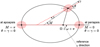 |
Fig. 1 Schematic representation of the pointing direction of the satellite’s long axis θ and thus of the orientation of the satellite-fixed frame, including the contribution of the longitudinal physical libration γ. The satellite is represented at periapsis (M = 0), at apoapsis (M = π), and at a arbitrarily chosen location along its orbit. In this work, we define the satellite-fixed reference frame such that the satellite’s long axis points towards the planet at apo- and periapsis. |
3.2.2 Mode decomposition of the tidal response
According to the linear theory of tides, the perturbed body’s response to a given tidal forcing mode is independent to forcings at other frequencies (provided that the body does not have lateral heterogeneities, see Rovira-Navarro et al. 2024), and can be described by a phase-lagged linear deformation. A purely linear deformation describes the body’s response to the static tide, while the phase lag accounts for the dynamical tide (i.e., not purely elastic response, see for example Efroimsky & Lainey 2007). Both the amplitude and phase of the deformation are frequency-dependent, as the body’s response to forcing (in terms of both how large the resulting deformation is, and how long it takes for the body to deform) depends on the frequency at which the forcing occurs, a behaviour described by the body’s rheology (see Section 4). The perturbed body’s response to the perturbing potential given by Eq. (25) therefore raises the following tide-induced potential, here evaluated at an external point r = (r, ϕ, λ) with r > R:
 (28)
(28)
Here the subscript t indicates that Ut is the tide-induced perturbation of the gravitational potential, and not the total gravitational potential U as in Eq. (28). The (frequency-dependent) static Love numbers kl(ωlmpqs) and phase lags ϵlmpqs describe the perturbed body’s gravity field deformation caused by the static and dynamical tides, respectively. The phase lags ϵlmpqs are often found alternatively parametrised by (frequency-dependent) tidal quality factors Q(ωlmpqs), defined as follows (e.g., Efroimsky 2012):
 (29)
(29)
In the simplified two-dimensional, degree-two response framework, the above expression can be further simplified as
 (30)
(30)
In the following and for the sake of conciseness, we drop the subscript l = 2. The above formulation and all subsequent developments can however be easily expanded to higher degrees if required.
All inclination functions Flmp(i) are O(i) except for  and F220(i) = 3 + O(i) (e.g., Efroimsky & Williams 2009; Boué & Efroimsky 2019). This allows us to further simplify the above expression by only keeping the terms lmpqs = 201qs (order zero response Ut,m=0) and lmpqs = 220qs (order two response Ut,m=2):
 (31)
(31)
 (32)
(32)
 (33)
(33)
The dominant forcing modes are defined as (Eq. (18))
 (34)
(34)
 (35)
(35)
or, in the specific spin-orbit resonance case (i.e., for tides raised on a synchronous satellite) (Eq. (27)) as
 (36)
(36)
The corresponding eccentricity functions G21q(e) and G20q(e) are provided in Table C.1. The forcing mode ω22000 is the only term in O(e0) and therefore typically dominates the body’s response. If the perturber is in a 1:1 spin-orbit resonance, however, this leading mode vanishes (q = s = 0 leading to ω22000 = 0 in Eq. (36), while  outside of the spin-orbit resonance). This is at the core of the complications arising when modelling the tides raised on a synchronous satellite, as will be discussed in Section 3.5.
Considering Eqs. (31)–(33) and the expression for the perturbed body’s static gravitational potential (Section 2.1, Eq. (4)), the tide-induced potential can alternatively be expressed as time-dependent variations to be added to the perturbed body’s static gravity field coefficients. For the degree-two response and in the two-dimensional case, the expected variations of the (unnor-malised) cosine and sine coefficients ∆C2m and ∆S2m are given by
 (37)
(37)
 (38)
(38)
 (39)
(39)
(see Section 3.1 on how to introduce these coefficient variations into the translational and rotational equations of motion).
The potential expansion leading to the above expressions for the deforming body’s gravity coefficients still relies on a number of simplifying assumptions which are important to keep in mind. First, Kaula’s expansion assumes that the semi-major axis a, eccentricity e, and inclination i of the perturber are constant (for expansion to time-varying eccentricity, see e.g., Walker & Rhoden 2022). Moreover, as highlighted above for the spin-orbit resonance case in the presence of librations, the quantities ωlmpqs, defined by the orbital elements and rotation rates  , and
, and  (Eq. (18)), can only be considered as forcing modes if they are secular (i.e., exhibit very slow variations). The two aforementioned conditions can be problematic for satellites trapped in mean motion resonances (MMRs) (e.g., Jupiter’s Galilean moons) because of the (rapid) periodic orbital element variations that the resonances induce. Finally, our present libration model only includes a single harmonic at the satellite’s orbital frequency (Eq. (20)). Further expansion of Eq. (25) to account for additional harmonics in the satellite’s librational response are discussed in Section 7.1 and Appendix D, but would come at the cost of increased complexity and computational load upon evaluation of the tidal potential.
3.3 Tidal torque
In this section, we focus on the tidal torque caused by tides raised on a synchronous satellite. This specific case requires more attention due to the vanishing of the leading tidal mode ω22000 and contribution of the physical libration(s), as high-lighted in Section 3.2. The torque induced by satellite tides is moreover essential to our understanding of the effect of satellite tides on the satellite’s own orbit (see Section 3.5). Similar derivations would provide equivalent expressions for the simpler case of planet tides where the leading tidal mode ω22000 does not vanish.
Starting from the libration-compatible expansion of the tidal potential given by Eq. (30), one obtains the following expression for the tidal torque, as done in Frouard & Efroimsky (2017). Because the torque only acts along the orbit normal, we directly provide its out-of-plane component:
 (40)
(40)
 (41)
(41)
with m ≥ 1 as the order zero response does not induce a torque. Keeping only the leading terms lmp = 220 (see Section 3.2.2 and eccentricity functions listed in Table C.1) with p′ = p = 0, the above eventually becomes
 (42)
(42)
The secular component of the tidal torque  can be recovered by only retaining the terms that fulfil the following condition:
 (43)
(43)
Other terms are periodic and cancel out over one orbital period. The second part of the above condition follows from the forcing mode ω220qs vanishing if β220qs = 0. Recalling the tidal forcing modes definition in the specific spin-orbit resonance case (Eq. (36)), this translates to4
 (44)
(44)
Summing all the terms fulfilling the above condition and simplifying the resulting expression eventually leads to
![Mathematical equation: ${{\bar \Gamma }_t} = 18{{G{m^{ \star 2}}{R^5}} \over {{a^6}}}{k_2}\left[ {{e^2}\sin {_n} + {{{\cal A}e} \over 2}\sin {_n}} \right],$](/articles/aa/full_html/2026/03/aa57439-25/aa57439-25-eq69.png) (45)
(45)
with ϵn the tidal phase lag evaluated at the once-per-orbit forcing frequency ωlmpqs = n. The first term of the secular torque Γ¯ corresponds to the zero-libration case, and the total tidal torque including the libration’s contribution can thus be re-written as
 (46)
(46)
where  is the tidal torque in the absence of libration.
3.4 Alternative force formulation
When including tidal effects in the orbital dynamics of a planet–satellite system, a commonly used approach is to translate the tidal potential (Eq. (28)) into a tidal force acting as an additional perturbation on the satellite, both for planet and satellite tides (e.g., Lainey et al. 2007; Lari 2018) (see discussion in Section 3.6 for more details on why such an alternative is necessary). The expression for this tidal force, evaluated at a point r from the perturbed body is the following (see derivation in Section 2.3.2 in Fayolle 2025):
![Mathematical equation: $\eqalign{& {\bf{F}}\left( {{\bf{r}},{{\bf{r}}^ \star }} \right) = - {m^ \star }\nabla {U_t}\left( {{\bf{r}},{{\bf{r}}^ \star }} \right) \cr & = - {3 \over 2}G{m^{ \star 2}}{R^5}{k_2}{\left( {{1 \over {{r^ \star }}}} \right)^2}{\left( {{1 \over r}} \right)^3} \cr & \left[ {\left( {1 - 5{{\left( {{{\bf{r}}^ \star }\cdot{\bf{r}}} \right)}^2}} \right)\widehat {\bf{r}} + 2\left( {{{\bf{r}}^ \star }\cdot{\bf{r}}} \right)\widehat {\bf{t}}} \right]. \cr} $](/articles/aa/full_html/2026/03/aa57439-25/aa57439-25-eq72.png) (47)
(47)
To model the effect of tides on the mutual orbit of the perturbed and perturbing bodies, F must be evaluated at the per-turber’s position: for planet tides, the tidal force represents the additional acceleration acting on the satellite due to the tides it raises on its central planet; for satellite tides, it is the reaction to the force acting on the planet due to planet-raised tides on the satellite. To account for the dynamic tide (i.e., not purely elastic response of the perturbed body), an important step in the typical derivation of the tidal force lies in the following relation between the perturber’s position when the tidal potential is raised r, and at the moment of the forcing r⋆ (Mignard 1980):
 (48)
(48)
Here ω is the rotation vector of the perturbed body and ∆t the so-called tidal time lag, i.e., the amount of time required for that body to deform due to the tidal forcing. ∆t relates to the tidal phase lag as
 (49)
(49)
with ϵ the phase lag at the main forcing frequency and T the period of this forcing. An important underlying simplification of this tidal force formulation is that it assumes a single frequency forcing and response, as well as a constant time lag, therefore neglecting the influence of the satellite’s eccentricity (so-called constant time lag model). Circling back to the general definition of the forcing modes (Eq. (18)), the nominal leading forcing mode is  , resulting in the following tidal period:
 (50)
(50)
This for instance corresponds the forcing period for the tides raised on the planet. For the specific case of the spin-orbit resonance (Eq. (27)), the leading forcing modes become ω22010 = n and ω220,−1,0 = −n, such that the tidal period is
 (51)
(51)
Using Eq. (48) to expand (1/r⋆)3 as a O(∆t2) expression eventually leads to the following expression for the tidal force, after decomposing the above into radial and tangential components and assuming the orbit’s normal and rotation pole are coplanar (for a complete derivation, see Mignard 1980),
 (52)
(52)
with  the time derivative of the true anomaly (i.e., the orbital velocity).
The typical formulation for the tidal force as given in Eq. (52) relies on a few important simplications:
a truncation at O(∆t2) (Eq. (48)), which might not be valid for large eccentricities;
a single-frequency forcing and response, as evidenced by the definition of the tidal time lag in Eq. (49) (equivalent to assuming a frequency-independent response to the leading term(s) in Eq. (30)).
While a more rigorous, frequency-dependent expression for the tidal force could be derived from Eq. (30), Eq. (52) has been widely and successfully used to model the effects of both planet and satellite tides in natural ephemerides applications, and proven suitable to reproduce the main features of tidally driven orbital evolution (Lainey et al. 2007, 2009, 2012, 2019, 2020). The effects of planet and satellite tides on their mutual dynamics, and the limitations of this tidal force formulation to model these effects in the specific spin-orbit resonance case will be elaborated upon in Section 3.5.
From the tidal force expression in Eq. (52), one can moreover recover the tidal torque derived from the tidal potential in Eq. (45), including the additional contribution of the physical libration. Recalling that the rotation rate of a synchronous satellite in the presence of one main once-per-orbit longitudinal libration is
 (53)
(53)
the tangential component of the tidal force (from which the tidal torque originates) can be re-written as
 (54)
(54)
 (55)
(55)
with Ftan|γ=0 the tangential component of the tidal force in the absence of physical librations. This matches the librational contribution obtained with the tidal potential approach (Eq. (46)).
3.5 Effects of planet and satellite tides on the satellite’s orbit
The loss of energy through tidal dissipation drives the evolution of a natural satellite’s orbit, and more specifically the changing rate of its semi-major axis and eccentricity. The literature provides well-known approximations for the secular evolution of a and e, with an important distinction between planet and satellite tides (e.g., Kaula 1964; Goldreich & Soter 1966; Peale & Cassen 1978; Peale 1999; Malhotra 1991; Lainey et al. 2009; Lari 2018; Emelyanov 2018; Boué & Efroimsky 2019). For the former, i.e., raised on the planet by the satellite, the resulting change in the satellite’s semi-major axis and eccentricity can be approximated by5
 (56)
(56)
 (57)
(57)
For the case of tides raised by the planet on a synchronous satellite, however, two conflicting secular variations of the moon’s semi-major axis can be found (e.g., Goldreich & Soter 1966; Lainey et al. 2009 vs Emelyanov 2018; Boué & Efroimsky 2019), as reported below6,
 (58a)
(58a)
 (58b)
(58b)
whereas they are consistent for the eccentricity changing rate:
 (59)
(59)
This apparent discrepancy for the effects of satellite tides finds its origin in the commensurability between the moon’s orbital and rotational periods, combined with the need to conserve rotational energy for the spin-orbit resonance to be maintained. A detailed explanation can be found in Magnanini et al. (2026), but the reasoning will be briefly reconstructed here, as it brings insights into the modelling challenges associated with satellite tides.
Evaluating the orbital energy dissipated through satellite tides in the case of exact synchronicity leads to the semi-major axis evolution given in Eq. (58b), a result that is equivalently obtained starting from the simplified force formulation in Eq. (52) or from the complete tidal potential expansion (Eq. (30)) (for a rigorous derivation of the orbital elements evolution from Kaula’s tidal potential expansion, see Boué & Efroimsky 2019; Magnanini et al. 2026). As shown in Section 3.3, however, exact 1:1 spin-orbit synchronicity implies a non-zero secular tidal torque (Eq. (45)). A slightly super-synchronous rotation rate can be computed for which the tidal torque cancels out over one orbit (Levrard 2008; Wisdom 2008),
 (60)
(60)
which can thus seem a more stable rotational state (no residual tidal torque spinning up the satellite’s rotation). For this pseudo-synchronicity case, the amount of tidal energy dissipation is no longer consistent with Eq. (58b), but one instead recovers the more commonly used approximation given by Eq. (58a) (see Section 2.3.4 in Fayolle 2025)7.
However, the exactly synchronous rotation of the Solar System’s natural satellites contradicts Eq. (60), and the physical realism of such a pseudo-synchronous equilibrium for terrestrial bodies was indeed refuted (e.g., Makarov & Efroimsky 2013). For natural satellites to maintain exact spin-orbit resonance, the secular tidal torque must nonetheless be compensated, as it would otherwise progressively speed up the satellite’s rotation out of spin-orbit synchronicity.
In practice, this torque balance is maintained via a slight re-orientation of the satellite (e.g. as theorised in Yoder & Peale 1981; Murray & Dermott 1999; Williams & Efroimsky 2012; Makarov & Efroimsky 2013): the body’s triaxiality causes a non-zero secular torque if the principal axis of inertia and the direction of the planet at periapsis are slightly misaligned (see Eq. (14) and Figure 1). To conserve spin-orbit resonance, the averaged torque exerted by the central planet on the non-spherical satellite  due to this misalignment (Eq. (14)) and the secular torque caused by satellite tides
  (Eq. (45)) should therefore cancel out,
 (61)
(61)
 (62)
(62)
thus leading to the following equilibrium S22 value (e.g., Magnanini et al. 2026):
 (63)
(63)
This non-zero S22 ensures constant rotational energy, but also causes a secular drift of the satellite’s semi-major axis, which exactly compensates for the discrepancy between Eqs. (58b) and (58a). This counterbalancing re-orientation of the satellite here translates into a non-zero S 22 because we choose to keep our body-fixed convention unchanged (i.e., satellite’s x-axis pointing towards the planet at apo- and periapsis, see Figure 1 and details in Section 5.2.2). As discussed in Section 2.1, it could equivalently be represented by a small rotation of the satellite-fixed frame8. Nevertheless, the counteracting triaxial torque caused by the satellite’s re-orientation and its subsequent effects on the dynamics are invariant upon different body-fixed frame conventions. Evaluating Eq. (63) for Io (the only Moon for which we have an estimate for k2/Q = k2 sin |ϵn| = 0.015, Lainey et al. 2009), the conservation of rotational energy requires a balancing S22 = 1.30 · 10−9, equivalent to an orientation offset of 6.67 · 10−5 rad.
The total semi-major axis rate of the satellite is therefore in agreement with Eq. (58a), irrespective of any assumption on exact or pseudo-synchronicity. The sole difference is that in the physically realistic case of fully synchronous satellites, only part of the total secular change in a directly results from the effect of tides on the orbit, while the other part is an indirect effect of the conservation of rotational energy and the resulting non-zero S 22 (and is thus oftentimes overlooked when focussing on orbital evolution).
Finally, it should be noted that Eqs. (58a) and (59) approximate the secular change in the satellite’s semi-major axis and eccentricity caused by satellite tides in the absence of librations. The amount of orbital energy dissipated when accounting for the influence of the main once-per-orbit longitudinal libration is
 (64)
(64)
with ∆Eγ and ∆Eγ=0 representing the energy dissipation with and without libration, respectively (see detailed derivation in Efroimsky 2018). This eventually leads to
 (65)
(65)
for the secular evolution of a and e caused by tides raised on a librating synchronous satellite, with  and
and  given by Eqs. (58a) and (59), respectively.
3.6 Implications for satellite tides modelling
As demonstrated in Section 3.5, accurately representing the effect of satellite tides on the dynamical evolution of a synchronous satellite requires the consistent modelling of its orbit and rotation for (i) the main tidal forcing mode ω22000 to vanish (Eq. (36)); (ii) the spin-orbit resonance to be maintained (Eqs. (61)–(63)). These two conditions are inter-dependent, and breaking one of them would eventually lead to breaching the other. Maintaining both above conditions is, however, very difficult to achieve in practice when relying on classical kinematic rotation models (i.e., analytical representations of the satellite’s rotation, with the possible incorporation of multi-frequency perturbations, see Section 2.1), as will be discussed in the following.
Due to the vanishing of the main tidal forcing mode ω22000 in Eq. (33), the secular evolution of the satellite’s orbital elements caused by satellite tides is dominated by linear functions of e2 (Eqs. (58a) and (59)). This implies that any model simplification that incurs an error in O(e2) is no longer acceptable and would violate the two aforementioned conditions (i.e., ω22000 = 0 while maintaining the resonance). This O(e2) consistency requirement is well illustrated by the conservation of rotational energy issue exposed in Section 3.5 and its implications to both maintain the spin-orbit resonance and predict the right secular evolution of the satellite’s semi-major axis (discrepancy between Eqs. (58a) and (58b)). The equilibrium between the secular tidal torque (Eq. (45)) and the restoring triaxial torque (Eq. (61)), and its consequences (additional contribution to the semi-major axis change rate and conservation of exact- rather than pseudo-synchronicity, Eq. (60)) are indeed all O(e2) effects, whose delicate balance is contingent upon the coherent modelling of the intricate coupling between orbit and rotation.
In practice, this level of orbit-rotation consistency is extremely difficult to achieve with a kinematic representation of the satellite’s rotation. Such analytical rotation models typically assume that the satellite’s long axis points towards the empty focus (Section 2.1). This assumption is actually a O(e2) approximation in itself (e.g., Murray & Dermott 1999), whose practical implementation oftentimes relies on an additional O(e2) simplification (see Eq. (7)). This demonstrates that relying on the orbit’s empty focus to define the satellite’s rotation is not compatible with the O(e2) modelling consistency requirement necessary to accurately model satellite tides, with the important implications for the predicted orbital migration rate evidenced in Section 3.5. In addition to the inadequacy of such an implementation shortcut, a more fundamental flaw in adopting an analytical rotation model stems from the satellite’s rotational inertia, which prevents its orientation from instantly matching the osculating orbit. The satellite’s rotation indeed follows the long-term evolution of the orbit, rather than adapting to immediate perturbations (see in-depth discussion in Martinez et al. 2025). This is critical to maintain spin-orbit resonance, but makes it extremely challenging to define a suitable time-dependent rotation model while concurrently propagating the (perturbed) orbital dynamics of the satellite.
When modelling the effect of satellite tides on the satellite’s own orbit using the tidal force formulation given in Eq. (52), a commonly used approach allows to circumvent this orbit-rotation consistency issue. It exploits the fact that the energy dissipated by librational tides over one orbit amounts to 4/3 of that dissipated by radial tides (Murray & Dermott 1999). This allows us to translate Eq. (52) into a scaled tidal force acting in the radial direction only, while getting rid of the  librational term where the dependency on the satellite’s rotation comes into play (e.g., Lari 2018):
 (66)
(66)
This approach is a very efficient and robust workaround to accurately represent satellite tides in an orbital propagation without the need for a fully consistent rotation, which is precisely what makes the tidal force formulation so appealing for orbital dynamics propagation (see detailed discussion in Fayolle 2025).
By design, this force formulation is, however, only suitable to model and/or estimate the averaged effects of satellite tides on the satellite’s own orbit (over one orbital period). It is, by contrast, inapplicable to represent their influence on the dynamics of a neighbouring spacecraft (whether in orbit, or performing a flyby), or for highly accurate propagations of the moon’s instantaneous dynamics. The latter is typically accounted for by modelling tides as additional time-variations of the deformed body’s gravitational potential, as described in Section 3.2 (e.g., Petit et al. 2010; Iess et al. 2012; Goossens et al. 2024; Park et al. 2025), a modelling approach that is extremely rotation-sensitive when applied to tidal effects on the satellite’s dynamics (Magnanini et al. 2026). Using different models to include tides in the moons’ and spacecraft’s dynamics would nevertheless be prone to discrepancies, especially since satellite tides affect the spacecraft in two ways: via the direct effect of the satellite’s deformed gravitational potential, and via the indirect contribution of the moon’s tidally perturbed orbit on the spacecraft’s motion. For planetary missions relying on a series of moons’ flybys (e.g., Cassini, Juice, Europa Clipper), addressing such a modelling challenge is therefore particularly critical, not only to ensure the consistent propagation of the satellites and spacecraft, but also to ultimately allow for the consistent estimation of tidal (and rotational) parameters from their combined effects on the moons’ and spacecraft’s orbits. This is especially important to avoid mismodelling the satellite’s expected orbital migration rate and therefore under- and over-evaluating the tidal dissipation because of any translational-rotation inconsistency (see Section 3.5).
The unique complications arising in the spin-orbit resonance case, combined with the need to consistently model tidal effects on both the satellite’s and spacecraft’s dynamics, call for a unified way to model the complex interplay between the satellite’s orbit, rotation, and tidal deformation. In particular, this requires accounting for the instantaneous tidal deformation of the satellite’s gravitational potential, in a manner that ensures full consistency between the tidal forcing and subsequent response.
4 Deformation model
Adopting the approach followed by Correia et al. (2014) and Boué et al. (2016) for exoplanetary systems, we propose to concurrently propagate the perturbed body’s translational and rotational dynamics, along with the instantaneous deformation of its gravitational potential caused by tidal effects. Such a three-level dynamical model (orbit, rotation, deformation), by automatically accounting for all couplings at play, ensures the full consistency of the propagation results while reproducing the main dissipation-driven dynamical evolution features (Sections 3.3 and 3.5).
While the complete set of equations (including the translational and rotational dynamics from Section 2) will be re-iterated in Section 5.1, the following section focusses on the missing component: i.e., the deformation model adopted for the satellite’s deformation to dynamical forcing. Section 4.1 first introduces the general deformation modelling framework necessary to describe the tidal deformation of the perturbed body as a differential equation. Section 4.2 then provides the exact formulation for the Maxwell rheology used in the rest of this work.
4.1 General formulation
This section presents the model used to describe the perturbed body’s gravity field deformation induced by a perturbing potential W. Following Correia et al. (2014), the total perturbing potential evaluated at a surface point R is here defined as the sum of the tide-raising potential Wt and centrifugal potential Wc, as
 (67)
(67)
 (68)
(68)
with Wt(R) being given by Eq. (15) and ω the perturbed body’s rotational rate vector. The gravitational potential U′ induced by the body’s deformation under the above perturbing potential is given by the convolution (e.g., Boué et al. 2016)
 (69)
(69)
where k2(t) is the complex degree-two Love number distribution. The total gravitational potential U′ differs from the tidally induced potential Ut as our coupled model also accounts for the centrifugal deformation. We here restrict ourselves to the degree-two (l = 2) perturbation and response, but the above could be expanded to higher degrees (see e.g., Boué et al. 2016). It is moreover important to keep in mind that the tidally induced potential resulting from Eq. (69) is actually equivalent to the expression already derived in Section 3.2.2 (Eq. (30)), but presents the critical advantage of not relying on a mode decomposition.
Eq. (69) is generally applicable when modelling gravitational deformation under a perturbing potential, the body’s specific response to different forcings based on its interior properties (i.e., rheology) being described by its Love number distribution k2(t). It remains valid for all eccentricities (thus circumventing the possible O(e2) inconsistencies mentioned in Section 3.6), and does not rely on a Fourier-like series similar to the one used by Kaula (1964), implying that the dynamical problem at hand needs not be decomposable into such an expansion, which might indeed not be the case for satellites in MMRs (see Section 3.2.2).
4.2 Maxwell rheology
A viscoelastic response is typically assumed for natural bodies, with the Maxwell rheology (equivalent to a viscous damper mounted in series with an elastic spring) being widely used among possible rheological models. This model presents the combined advantages of offering a very simple mathematical formulation, while still adequately representing the main features of tidal dissipation (Boué et al. 2016). In the rest of this work, we therefore assume that both the planets and satellites under consideration behave as Maxwell bodies. The implications of such a modelling assumption will be discussed in Section 8. For a Maxwell body, the Fourier transform of the complex Love number distribution is (e.g., Henning et al. 2009)
 (70)
(70)
with  the body’s fluid Love number of degree two, and τ and τe the global and elastic (or Maxwell) relaxation times, respectively.
This Fourier transform turns the convolution in Eq. (69) into the following differential equation for the deformation-induced potential U(R) (adapted from Correia et al. 2014; Boué et al. 2016)
 (71)
(71)
 (72)
(72)
with Ueq the equilibrium deformation-induced potential (i.e., gravitational potential due to the body’s fluid response), defined as
 (73)
(73)
The dependency on t is made implicit in Eqs. (71)–(73) compared to Eq. (69).
Recalling the spherical harmonics expansion of the gravitational potential (Eq. (4)), the deformation-induced potential can be represented by time-dependent increments of the perturbed body’s gravity field coefficients. Owing to the orthogonality of spherical harmonic basis functions, the coefficient increments follow the differential equation for the deformation-potential (Eq. (72)):
 (74)
(74)
 (75)
(75)
with ∆C2m, ∆S2m and  the instantaneous and equilibrium coefficients, respectively. The latter can be directly derived from the equilibrium potential Ueq (Correia et al. 2014):
![Mathematical equation: $\Delta C_{20}^{eq} = - {k_f}\left[ {{{{{\dot \theta }^2}{R^3}} \over {3\mu }} + {1 \over 2}{{{\mu ^ \star }} \over \mu }{{\left( {{R \over {{r^ \star }}}} \right)}^3}} \right],$](/articles/aa/full_html/2026/03/aa57439-25/aa57439-25-eq111.png) (76)
(76)
 (77)
(77)
 (78)
(78)
Here  corresponds to the rotational rate, as the rotational velocity vector
  is perfectly aligned with the orbit’s normal in our simplified two-dimensional case. These equilibrium coefficients act as a forcing in the differential equations driving the time evolution of the gravity deformation (Eqs. (74)–(75)). From Eqs. (77)–(78), their time derivatives can be computed as follows:
![Mathematical equation: $\Delta \dot C_{20}^{eq} = k_2^f\left[ {{{2\dot \theta {R^3}} \over {3\mu }}\ddot \theta - {3 \over 2}{{{\mu ^ \star }} \over \mu }{{\left( {{R \over {{r^ \star }}}} \right)}^3}{{{{\dot r}^ \star }} \over {{r^ \star }}}} \right],$](/articles/aa/full_html/2026/03/aa57439-25/aa57439-25-eq116.png) (79)
(79)
![Mathematical equation: $\Delta \dot C_{22}^{eq} = - {{k_2^f} \over 4}{{{\mu ^ \star }} \over \mu }{\left( {{R \over {{r^ \star }}}} \right)^3}\left[ {3{{{{\dot r}^ \star }} \over {{r^ \star }}}\cos 2{\lambda ^ \star } + 2{{\dot \lambda }^ \star }\sin 2{\lambda ^ \star }} \right],$](/articles/aa/full_html/2026/03/aa57439-25/aa57439-25-eq117.png) (80)
(80)
![Mathematical equation: $\Delta \dot S_{22}^{eq} = - {{k_2^f} \over 4}{{{\mu ^ \star }} \over \mu }{\left( {{R \over {{r^ \star }}}} \right)^3}\left[ {3{{{{\dot r}^ \star }} \over {{r^ \star }}}\sin 2{\lambda ^ \star } - 2{{\dot \lambda }^ \star }\cos 2{\lambda ^ \star }} \right].$](/articles/aa/full_html/2026/03/aa57439-25/aa57439-25-eq118.png) (81)
(81)
Using the Darwin-Radau approximation, the fluid Love number and relaxation times are all related to the body’s interior properties (Correia et al. 2014):
 (82)
(82)
 (83)
(83)
 (84)
(84)
where ρ is the mean density, µ the shear modulus (i.e., rigidity), and η the viscosity. For a spherical body of constant density, the global relaxation time τ becomes
 (85)
(85)
It should be noted that the above definitions for the fluid Love number and relaxation times assume a homogeneous and incompressible body, and can therefore only describe the effective or averaged response of a body’s (stratified) interior. The implications and limitations of such an assumption will be discussed in Section 8. We nonetheless emphasise that they only affect the specific formulation of the differential equations for the gravity coefficients, and not the general framework of our coupled model. From Eq. (70), the (frequency-dependent) modulus and argument of a Maxwell body’s complex Love number can moreover be linked to the quantities k2(ω) and ϵ(ω) typically used in tidal potential expansions (Section 3.2) as follows:
 (86)
(86)
 (87)
(87)
This allows us to evaluate the body’s Maxwell response to tidal forcings at the different modes ωlmpqs, enabling a direct comparison between the results of our numerical propagation and the analytical formalism presented in Section 3.2. The incorporation of the deformational Equations (74)–(75) in the rest of our dynamical model will be discussed in Section 5.1.
It should be stressed that Eqs. (76)–(81), once inserted back in Eqs. (74)–(75), provide a specific formulation of the first order differential equation governing the gravity deformation, valid in our two-dimensional, zero obliquity case with limited perturbations. For high-accuracy applications, this simplified framework could however easily be expanded to more complex configurations. More specifically, generalising the above to three-dimensional problems would require foregoing the zero latitude assumption in the tidal potential formulation (Eq. (28)) and subsequently including order 1 coefficients ∆C21, ∆S21 in the propagation ( if ϕ⋆ ≠ 0). Eq. (72) can moreover easily be adapted to incorporate extra perturbations (e.g., third-body effects) in the gravitational deformation forcing in addition to the tidal and centrifugal potentials (thus modifying the equilibrium coefficients definition) and can be expanded to higher degrees.
5 Complete coupled model formulation and set-up
This section provides a detailed description of the propagation set-ups used to implement and test our coupled model, as well as an overview of the dynamical features and quantities to compare to classical models. Section 5.1 first provides the complete set of equations of motion to be integrated in our coupled model framework and highlights their interdependencies. Section 5.2 then presents the strategy required to identify a consistent, physically realistic initial state for our coupled dynamics.
To investigate the behaviour of our coupled translational-rotational-tidal approach, we use both the Earth–Moon and Mars–Phobos systems as test cases, paying special attention to the model’s ability to reproduce the dynamical evolution of a planet – synchronous satellite system caused by satellite tides. Section 5.3 describes the specific dynamical environment and propagation settings used for the two planet–satellite systems. We underline that our analyses do not aim to provide a complete and fully realistic dynamical descriptions of the systems under consideration, but rather to analyse the dynamical properties that naturally emerge from our coupled propagation, with special attention paid to tidal dissipation features. The main dynamical features that we expect our unified model to reproduce, outlining the scope of our model validation, are listed in Section 5.4.
All our simulations have been performed using the TU Delft Astrodynamics Toolbox (Dirkx et al. 2022, 2025). For this work, Tudat has been extended with the numerical integration of the gravity field in Eq. (93), building upon the existing functionality for coupled orbital-rotational dynamics of natural satellites (Martinez et al. 2025). Tudat has previously been applied to various studies in the modelling and estimation of natural satellite dynamics (e.g. Dirkx et al. 2016; Fayolle 2025).
5.1 Complete set of equations of motion
We here combine the orbit, rotation, and gravitational deformation models (separately presented in Sections 2.1, 2.2, and 4, respectively) into the complete set of equations forming our coupled model. The complete propagated state is defined as:
 (88)
(88)
where r, q, and z respectively represent the body’s translational, rotational, and gravitational states, the latter combining the propagated degree-two coefficients9 z = (∆C20 ∆C22 ∆S22)T (see Section 5.2.2 for the coefficients decomposition into static and time-varying components). Under the gravitational influence of a perturber ⋆, the time derivative of this extended state (in the perturber-centred frame) obeys the following set of equations of motion:
 (89)
(89)
 (90)
(90)
 (91)
(91)
 (92)
(92)
 (93)
(93)
Following the notations introduced in Section 2.1, ∇U and  represent the gradients of the perturbed and perturbing bodies’ gravitational potentials10 in their respective body-fixed frames (linked to the inertial frame via the rotation matrices RI/ and RI/⋆). Both gravitational potentials U and
  can be expressed using the formulation given by Eq. (4) (expanded to degree two in this work), but the gravity field coefficients of the deforming body are now time-varying, and are actually described by the gravitational state z. Finally, zeq designates the equilibrium coefficients vector (Eqs. (76)–(78)).
The coupling between the translational, rotational, and tidal dynamics is immediately apparent from the above set of equations, which all depend on the perturber’s body-fixed position and on the gravity coefficients of the deforming body. In particular, the perturbed gravitational potential of the body undergoing tides U(r, q, z) automatically accounts for the contribution of tidal deformation to the translational and rotational dynamics of the system. The orbital elements’ evolution and emergence of a secular tidal torque therefore naturally follow from the propagation of the tidally perturbed equations of motion (assuming a suitable initial condition of the dynamical system, see Section 5.2.1). This is a crucial distinction with respect to Sections 3.3 and 3.5 where they are separately computed from an additional tidal potential.
It is furthermore important to remark that  depends on the time derivative
  of the gravity coefficients, by definition of the inertia matrix (Eq. (11)). Conversely, the time derivative of the equilibrium coefficients
  depends on the time derivative of the perturber’s body-fixed longitude
  (Eqs. (79)–(81)), which in turn is a function of the time derivative of the angular velocity vector
  . These interdependencies between the time derivatives of the rotational and gravitational states should be carefully considered when implementing the above equations, and again highlight the need for a concurrent integration.
As a brief summary of the advantages and implications of the unified modelling approach described above with respect to classical decoupled models:
our concurrent propagation provides the body’s instantaneous gravitational deformation under the perturbing potential(s) (here tidal and centrifugal), that deformation being inherently consistent with the translational and rotational dynamics of the system. This allows tides to be consistently incorporated in the dynamics of both the satellite and a nearby spacecraft, while automatically accounting for the effects of any variation in the satellite’s rotation;
all instantaneous forcings (at all frequencies) are automatically incorporated in the equilibrium potential Ueq induced by the deformation (Eq. (73));
this approach does not involve any series expansion of the tidal potential, and therefore does not introduce any assumption regarding the secular rates of the satellite’ orbital elements, or any series truncation error (especially truncations in eccentricity).
5.2 Obtaining a realistic initial state
While our coupled model automatically ensures that the translational, rotational, and tidal dynamics remain fully consistent during the propagation, its ability of produce realistic dynamics for a given known planet–satellite system depends on the definition of a suitable initial state. This is especially critical in a propagation framework such as the one presented in this paper. As opposed to real data fitting, in a propagation-only set-up, there is no observation constraint forcing the system to follow its present dynamical state. In particular, two important points of attention arise which are specific to our fully coupled approach:
the propagated dynamics should not be corrupted by the artificial introduction of rotational normal modes (Section 5.2.1);
the mean gravity coefficients that the coupled model converges to should match our present knowledge of the satellite’s gravity field (Section 5.2.2).
The initialisation process adopted in this work (see detail in Section 5.2.3) relies on a long relaxation phase until the system’s dynamics reach a converged, physically consistent steady state (ensuring that the two above conditions are fulfilled, among others). The numerical integration of the tidal deformation makes this relaxation phase crucial: the propagation first undergoes a transient phase during which the gravity coefficients progressively converge to their mean equilibrium values.
5.2.1 Normal modes damping
Integrating the equations of motion for the rotational dynamics gives rise to resonant oscillations of the body-fixed principal axes, referred to as normal modes (e.g., Borderies & Yoder 1990; Rambaux et al. 2010). The frequency at which these normal modes occur is directly linked to the body’s interior properties. Specifically focussing on the orientation of the body’s long axis in our two dimensional case, the longitudinal normal mode frequency is given by (e.g., Rambaux et al. 2012)
 (94)
(94)
with Ixx, Iyy, Izz the diagonal elements of the inertia matrix (which are function of the degree-two gravity coefficients, see Eq. (11)) and n the orbit’s mean motion.
These resonant oscillations are typically damped over planetary system evolution timescales, and no longer affect the rotational dynamics of the Earth–Moon and Mars–Phobos systems under consideration. Numerically propagating the rotational equations of motion from an insufficiently judiciously defined, undamped initial state will, however, automatically introduce the normal modes in the resulting numerical solution of the equations of motion (Martinez et al. 2025). The interdependency between the normal mode’s frequency (Eq. (94)) and the gravity coefficient values makes the obtention of a damped initial state particularly critical when concurrently propagating a body’s rotation and gravitational deformation.
To make ensure that the non-physical oscillations originating from the normal modes are absent from our integrated rotational solution, we applied a similar damping algorithm as done in Rambaux et al. (2012) or Martinez et al. (2025) (among others). This algorithm relies on the addition of an artificial damping torque to Eq. (10),
 (95)
(95)
with τd a damping timescale. This torque forces the body to maintain its (known) mean rotation ω0 while damping other rotational responses (for more details, see e.g. Rambaux et al. 2012; Martinez et al. 2025). Once a damped initial state (i.e., no longer affected by normal modes) has been obtained, Γdamping is removed, and the coupled translational-rotational-tidal dynamics are re-propagated from this damped initialisation.
5.2.2 Gravity deformation conventions and set-up
An important aspect of our model set-up relates to the distinction between the static and varying parts of the perturbed body’s gravity field. The fluid number of a uniform body in hydrostatic should theoretically be equal to 3/2. However, both the Moon and Phobos are known to depart from this exact uniform hydrostatic state. We chose to define the fluid number kf such that it matches our current knowledge of these moons’ C20 values using Eq. (82). Despite this particular set-up choice, the equilibrium deformation described by Eqs. (76)–(78) cannot exactly reproduce our present estimates of the satellite’s degree-two gravity coefficients. Eqs. (76)–(78) indeed cannot (entirely) account for the non-hydrostatic part of the satellite’s gravity field, even with a scaled kf value. It should nonetheless be noted that, provided that one can find an appropriate Maxwell rheology law (Eq. (70)) to describe the body’s response to forcing, this limitation does not hinder the ability of our coupled model to produce a realistic deformation response and consistently account for the dynamical signatures of said deformation.
However, to ensure that the deforming body’s gravitational potential is in agreement with its known gravity coefficients once the equilibrium deformation (Eq. (73)) is reached, we defined a base static gravity field to which the deformation propagated with Eqs. (74)–(75) is added. The instantaneous gravity coefficients are thus given by
 (96)
(96)
 (97)
(97)
Here ∆C2m(t) and ∆S 2m(t) are the coefficient variations numerically integrated with Eqs. (74)–(75), their equilibrium values being given by Eqs. (76)–(78).  and
and  , on the other hand, describe the static part of the gravity field (including the non-hydrostatic component). When initialising our model, these static coefficients were computed by subtracting the equilibrium deformation (Eqs. (76)–(78), evaluated at initialisation) from the body’s known coefficients (noted C2m and S2m), as follows:
 (98)
(98)
 (99)
(99)
It is important to keep in mind that this set-up choice was only intended to keep our physical representation of the deformed body (either the Moon or Phobos) aligned with our present knowledge of that body’s gravity field, but does not affect our modelling of the tidal response.
In our coupled model, the tidal deformation is tied to the definition of the body’s rheology. The Maxwell model used in our coupled framework is parametrised by three quantities (Section 4.2): the fluid Love number kf, and the two relaxation times τ and τe (see Eq. (70)). As mentioned in Section 3, classical models assume a single-frequency forcing and response, such that current estimates of tidal parameters for natural satellites (if available) are therefore also quantified at a single-frequency, the Moon being a notable exception (e.g., Williams & Boggs 2015). To define appropriate relaxation times, we assumed that the values available (if any) for the body’s k2 and Q parameters correspond to the leading forcing frequency (i.e., |ω22010| = n for a synchronous satellite, see Section 3). Using Eqs. (86) and (87) evaluated at that leading forcing mode, one can determine the corresponding τ and τe quantities. Specific values for the tidal parameters and relaxation times of the Earth–Moon and Mars–Phobos systems are provided in Section 5.3.
Finally, the definition of a common convention for the satellite-fixed reference frame is critical to ensure the consistent analysis and interpretation of our results, especially since we concurrently propagate both the moon’s rotation and its gravity field (defined in the body-fixed frame). Theoretically, the body-fixed reference frame can be arbitrarily chosen without any impact on the results (see Section 2.1). However, for ease of interpretation and to make our model and results consistent with classical tidal theory conventions, we defined it in such a way that the longitude of the central planet in the satellite-fixed frame is equal to zero once averaged over an integer number of orbits, following the conventional definition of a synchronous orbit (see Figure 1). In the following sections, all our results are provided in this particular moon-fixed frame. The choice of a specific reference frame would not be as critical in the simpler case of planet tides, in the absence of the 1:1 commensurability between the tidal and rotational frequencies.
Nominal Earth–Moon and Mars–Phobos system parameters and integration settings.
5.2.3 Initialisation procedure overview
The three constituents of the coupled model’s propagated state (translational, rotational, and gravitational, see Eq. (88) in Section 5.1) were initialised as follows:
translational state at initial epoch taken from the satellite’s ephemeris;
rotational state defined by initially assuming a simple synchronous rotation model (here with the long axis of the satellite exactly pointing towards the empty focus), with zero obliquity (thus directly constrained by the translational state);
gravitational state set to the coefficients’ equilibrium values
 .
.
The exact equilibrium state to which the coupled model will converge is, by definition, not known prior to the propagation. Nevertheless, an initial estimate can be obtained by inserting the chosen initial translational–rotational state into Eqs. (76)–(78). We note that initialising the propagated gravity coefficients close to their expected converged values is not an absolute requirement for a realistic initialisation, but speeds up the process by shortening the transient phase necessary for the coupled model to reach a converged gravitational state. The static gravity coefficients and Maxwell model parameters were defined as described in Section 5.2.2, ensuring that this converged state is consistent with our present estimates of the satellite’s gravity field.
Starting from the initial state defined above, we first proceeded with the removal of the rotational normal modes by propagating the planet–satellite system with an additional damping torque, as detailed in Section 5.2.1. For both the Earth–Moon and Mars–Phobos test cases, this initial damping phase was conducted over five times the nominal propagation durations reported in Table 1. Following this damping process and still as part of the initialisation procedure, we further extended the relaxation phase to ensure that:
removing the artificial damping torque did not re-introduce normal modes’ signatures;
the dynamical system reached convergence (evaluated by monitoring variations in the gravity coefficients’ mean values).
The initialisation process described above is specific to the propagation-only scope of this study. If eventually extended to an estimation framework allowing for fitting either to real data or to a reference ephemeris solution, a physically realistic initialisation of the coupled model would be naturally informed by the observational constraints. These constraints would guide the determination of initial conditions that, upon propagation, lead the model to reproduce the dynamical system under consideration.
5.3 The Earth–Moon and Mars–Phobos systems as test cases
All relevant quantities describing our dynamical environments for the Earth–Moon and Mars–Phobos systems are reported in Table 1. They correspond to a simplified representation of the actual systems (e.g., two-dimensional, gravitational potential and deformation expanded to degree two only). For the Earth–Moon system in particular, such a simplified set-up is well below the level of fidelity necessary to support millimeter-accuracy LLR (Lunar Laser Ranging) ephemerides applications. While perfectly suited to the scope of our modelling consistency analysis, turning our propagation set-up into an operational ephemeris model would require including three-dimensional effects and relevant perturbations such as third-body and figure-figure interactions. The necessary extensions to our current implementation of the gravity deformation differential equations were briefly sketched in Section 4.2.
Finding a suitable initialisation for our coupled propagation proved more challenging for the Mars–Phobos system. This is a result of Phobos’ strong triaxiality and small distance to Mars, combined to its longitudinal normal mode being close to the leading forcing frequency, which together make this system more dynamical complex. A more detailed discussion of our model set-up for the Mars–Phobos case and its (absence of) implications regarding tidal modelling, which this paper primarily focusses on, can be found in Appendix A.
Regarding the rheological model, the nominal relaxation times for the Moon were chosen to match the k2 and Q values as given in Lainey (2016). For Phobos, no estimate for k2 and Q is currently available (see e.g., wide range of k2/Q values used in Bagheri et al. 2021). As an alternative, we considered the range of possible k2 values (k2 ∈ [2 · 10−7; 5 10−4]) provided in Le Maistre et al. (2013) based on realistic interior models. We arbitrarily chose k2 = 1.3 · 10−4 and Q = 37.5, (the latter matching the Moon’s value). For both the Moon and Phobos, we also tested the behaviour of our coupled model for different relaxation times, varying the ratio between the global and Maxwell relaxation times from τ/τe = 1 to 200.
For the Moon, the expected amplitude of the physical libration as calculated from Eq. (21) is very small ( ), especially in light of the Moon’s relatively large eccentricity, the ratio
  driving the librational contribution to tidal dissipation effects (Eqs. (46) and (65)). For Phobos, on the other hand, the once-per-orbit physical libration is much larger than the Moon’s, with a ratio
  . As discussed in Efroimsky (2018), this indicates that the enhancement of tidal dissipation caused by librations is far from negligible in Phobos’ case.
5.4 Scope of our coupled model validation
To validate our unified orbital-rotational-tidal model, the following dynamical features, which are all derived from the tidal theory described in Section 3, are critical to investigate:
the secular evolution of the satellite’s orbital elements da/dt and de/dt, which should match Eqs. (58a) and (59) for satellite tides, respectively;
the agreement between the gravity coefficients’ increments as numerically propagated by Eqs. (74)–(75), and analytically derived from the tidal potential expansion (Eqs. (37)–(39));
the respect of exact synchronicity, which implies recovering Eq. (19);
(i) the equilibrium between triaxial and tidal torques, thus conserving rotational energy (Eq. (61)); and (ii) the emergence of the expected non-zero static S22 coefficient (Eq. (63)) to ensure (i);
the expected contribution of physical librations to the satellite’s translational-rotational evolution (Eqs. (45) and (65)), most noticeable in the Mars–Phobos case (see Section 5.3).
These points cover the main effects of tidal dissipation on the translational-rotational evolution of the system, and thus provide a comprehensive validation framework for our model. It should be noted that the above quantities and/or dynamical features that we compare our model against in Sections 7.1 and 7.2 follow from tidal theory analytical predictions (see Section 3). In our unified model, however, they are direct outputs of the coupled propagation, and as such do not rely on underlying derivation simplifications or modelling assumptions. We finally recall we here limit ourselves to a simplified, two-dimensional system. The extension of our model to more realistic cases will nonetheless be discussed in Section 8. We moreover focus on the effects of tides raised by the planet on a synchronous satellite.
6 Propagation results
We propagated the coupled equations of motion (Eqs. (87)–(90)) to model the effects of tides raised on the satellite for both the Earth–Moon and Mars–Phobos systems, using the nominal propagation settings reported in Sections 5.3 and 5.4, respectively. Each propagation was first preceded by an initialisation process (outlined in Section 5.2.3), including a damping step to remove the effects of the rotational normal modes from the dynamics (Section 5.2.1). The results of the damping algorithm demonstrating the successful attenuation of the normal modes can be found in Appendix B. The following sections focus only on the results of the damped dynamics propagation.
The uniqueness of our coupled approach lies in the numerical integration of the tidal deformation, such that we obtain time variations of the satellite’s degree-two gravity field coefficients as part of the solution of the equations of motion, in addition to its translational and rotational states (see extended state definition in Eq. (88)). Before investigating the tidal signatures in the dynamics, we here describe the time evolution of these three types of dynamics obtained from the propagation.
6.1 Gravity field deformation history
First focussing on the satellite’s gravity field deformation, Figure 2 displays the integration results for the coefficient variations ∆C, S2m for both the Moon and Phobos. We plot the deformations obtained over the entire propagation duration as a function of the mean anomaly M, such that the results shown in Figure 2 actually span over many orbital periods. Both the Moon’s and Phobos’ gravity coefficient variations follow similar, once-per-orbit patterns, which also remain unchanged over a large number of orbits, as expected for satellites in spin-orbit resonance. ∆C20 and ∆C22 are both dominated by a cosine-shaped function with a period of one orbit, reaching its minimum around periapsis and maximum around apoapsis for ∆C20 (with a small angle lag with respect to exact peri- or apo-apsis due to dissipation, see Section 3), and vice versa for ∆C22. ∆S22, on the other hand, primarily exhibits a sine wave behaviour. This is consistent with the tidal deformation forcing acting on each of these coefficients, represented in our equations by the equilibrium gravity coefficients (Eqs. (76)–(78)).
To gain more insights into the spectral content of the propagated gravity field deformations beyond the dominating once-per-orbit response immediately observable in Figure 2, we performed a Fast Fourier Transform (FFT) decomposition of the coefficients, provided in Figure 3. In addition to the leading once-per-orbit signature, the FFTs of the gravity coefficient variations all display strong peaks at each higher harmonic of the orbital period. This is in agreement with the main forcing modes derived from Kaula’s tidal potential expansion (Eq. (27)), which all coincide with harmonics of the anomalistic mean anomaly rate, equal to the averaged mean motion in the spin-orbit resonance case. A refined analysis of the gravitational deformation response, including a detailed comparison with the tidal potential expansion theory outlined in Section 3, will be provided in Section 7.1. Finally, the absence of a noticeable FFT peak at the normal mode frequency demonstrates that the normal modes in the satellite’s rotational dynamics have been sufficiently damped (see Appendix B).
 |
Fig. 2 Propagated gravity field time variations for the Moon (red) and Phobos (purple) over the entire propagation duration, thus spanning over many orbital periods which here overlay perfectly. |
 |
Fig. 3 Fourier transform of the propagated gravity field coefficient variations (panel a: Moon ; panel b: Phobos). The dashed vertical black lines indicate the mean motion frequency and higher harmonics, while the dashed red line delineates the normal mode frequency. |
6.2 Time evolution of the satellite’s rotational dynamics
A crucial aspect to consider when investigating the physical realism of the propagated dynamics is the conservation of the spin-orbit resonance. As discussed in Section 3.5, this is mutually critical to the coherent modelling of tidal effects and rotation: maintaining the resonance is a necessary condition to consistently model the effects of satellite tides on the dynamics but, conversely, is also contingent upon the accurate representation of such tidal effects. This is therefore a particularly important validation criterion, especially since classical, decoupled modelling approaches are known to be prone to rotation-tides inconsistencies (see Section 3.6).
Using Phobos as a test case (because of its large physical libration), Figure 4a displays the longitudinal libration extracted from our propagation as a function of mean anomaly, again over the entire propagation duration. The fact that the once-per-orbit behaviour of the longitudinal libration remains constant over a larger number of orbits demonstrates that the spin-orbit resonance is indeed conserved. Furthermore, the propagated gravity coefficients are also good indicators for whether the satellite’s rotation is moving out of spin synchronicity, given their strong sensitivity to the body-fixed longitude of the central planet λ⋆ (Eqs. (76)–(78)). A progressive de-synchronisation would indeed affect the time evolution of the body-fixed longitude, which would eventually be reflected in the propagated gravity coefficients history. The fact that the behaviour of the coefficient variations as a function of M remains unchanged over the entire propagation (Figure 4a) thus also brings confidence in our coupled propagation maintaining spin-orbit resonance.
Figure 4b finally provides the FFT decomposition of Phobos’ physical longitudinal libration. As expected, the peak frequencies match those of the gravitational response, with forcings occurring at harmonics of the orbital frequency. While the amplitude of the once-per-orbit physical libration is in agreement with the theoretical expectation given by Eq. (21), the multi-frequency FFT spectrum evidences the inherent limitation of a single-frequency librational model as described by Eq. (20). The importance of the additional librational forcings observed in Figure 4b for the tidal response will be further discussed in Section 7.1.
6.3 Time evolution of the satellite’s orbital elements
Now considering the satellite’s orbital dynamics, Figure 5 displays the propagation history of the Moon’s semi-major axis and eccentricity (similar results were obtained for Phobos). Both exhibit large periodic variations, superimposed with a negative secular trend (which other orbital elements do not display). Our translational dynamics model include the mutual gravitational accelerations between the satellite and its central planet (Section 2.1) and, as such, automatically accounts for the effect of the (numerically integrated) tidal deformations as part of these gravitational interactions.
In the absence of tidal dissipation (i.e., when setting τ = τe, see Section 4.2), the secular trends observed in a(t) and e(t) disappear. The remaining periodic variations are caused by the gravitational interactions between the static parts of the satellite’s and planet’s extended gravity fields, including the contribution from the static tides raised on the satellite. As expected, the clear secular evolutions of both the semi-major axis and eccentricity observed in Figure 5 can thus be entirely attributed to the dissipation of orbital energy due to tides. The quantitative values for the inwards migration and circularisation rates of the satellite’s orbit caused by its own tides will be further discussed in Section 7.2, where the results of our numerical propagation will put in perspective with analytical predictions from tidal theory (Section 3.5).
 |
Fig. 4 Physical libration extracted from Phobos’ coupled propagation. Panel a: Phobos’ libration as a function of mean anomaly (left y-axis). The red line is directly extracted from the coupled propagation, while the orange dashed line describes the single-frequency libration model (Eqs. (20) and (21)). The purple line (right y-axis) shows the difference between the two, dominated by the twice-per-orbit libration. Panel b: FFT of Phobos’s libration. The dashed vertical black lines indicate the mean motion frequency and higher harmonics, while the dashed red line delineates the normal mode frequency. |
 |
Fig. 5 Secular evolution of the Moon’s semi-major axis (panel a) and eccentricity (panel b) caused by its own tidal deformation. |
7 Discussion
Building upon the description of the propagation results in Section 6, we now put the observed tidal deformation of the satellite (Section 7.1) and its subsequent effect on the dynamics (Section 7.2) in perspective with what tidal theory predicts. Finally, Section 7.3 briefly discusses the coupled model’s results when investigating the effects of planet tides on the satellite’s orbit.
7.1 Tidal deformation
As indicated by the analytical frequency decomposition of the tidal response (Eqs. (37)–(39)), and further evidenced by the FFT of the propagated gravity coefficients (Figure 3), the tidal deformation of a given body can be reconstructed as a superimposition of its gravity field’s response to various forcings, which for a synchronous satellite occur at harmonics of the orbital frequency (Eq. (36)). In our coupled model, all forcing frequencies are automatically accounted for in the equilibrium potential Ueq(R) (Eq. (73)) and thus in the forcing equilibrium coefficients (Eqs. (74)–(75)).
To investigate the behaviour of our coupled model and specifically the propagated time variations of the satellite’s gravity coefficients, we started by evaluating the satellite’s rheology (Eqs. (86) and (87)) at the main tidal forcing frequencies ω220qs (Eq. (36)). The satellite’s Maxwell response is described by Figure 6 (using Phobos as an example). This highlights the strong frequency-dependency of the tidal dissipation (parametrised by the phase lag ϵ), underlining the limitations of single-frequency modelling approaches (see Section 3.4).
Plugging these frequency-dependent Love numbers k2(ω220qs) and phase lags ϵ220qs into Eqs. (37)–(39) allows us to compare how the gravity field variations predicted by the tidal potential theory match our numerically propagated gravity coefficients. In the following, the observed discrepancies between the propagated and predicted coefficients are referred to as gravity coefficient differences and designated by δC, Slm:
 (100)
(100)
This comparative analysis can only be performed for ∆C22 and ∆S 22. For ∆C20, the gravity field response predicted by Eq. (37) only accounts for the effect of the perturbing tidal potential, while omitting the contribution of the centrifugal potential, which is included in our coupled propagation (Eq. (67)). This represents another argument in favour of a coupled modelling approach, where additional forcings can easily be incorporated without resorting to an expanded, more complex perturbing potential expansion.
First focussing on the libration-free response (s = 0, see Section 3.2), the gravity coefficient differences are displayed in orange in Figure 7. The small differences demonstrate the good agreement between our propagation results and the tidal theory (Eqs. (38)–(39)). For the Moon’s case, where the librational contribution is expected to be very small (see Table 1), the amplitude of the difference between propagated and predicted coefficients amounts to about ∼0.1% of the total amplitude of the gravity coefficient variations (the coefficients’ absolute values and differences being both dominated by the once-per-orbit signature, see Figure 7). In Appendix C, we also separately provide the amplitudes of the gravity coefficient variations for each mode, as predicted by Eqs. (38)–(39) (Table C.2). This gives a quantitative indication of how much each tidal forcing mode contributes to the total tidal deformation. The FFT exhibits residual peaks at harmonics of the orbital frequency related to the librational signatures in the satellite’s rotation, as will be discussed in the following.
Including the contribution of the once-per-orbit longitude libration (Eq. (20)) into the predicted spherical harmonics expansion of the satellite’s deformation (s , 0 terms in Eqs. (38)–(39)) notably improves the gravity coefficient differences, as shown by comparing the orange (without libration) and purple (with once-per-orbit libration) in Figure 7. While already noticeable for the Moon, the improvement is strongest for Phobos, whose large libration significantly contributes to the tidal deformation. Accounting for the librational effect brings the amplitude of the gravity differences from ~27% to ∼0.2% of the total amplitude of the gravity coefficients variations. The contribution of the once-per-orbit libration to the body’s deformational response at each forcing is also reported in Appendix C (see Table C.2).
Considering the libration-expanded potential in Eq. (25), it is important to note that each orbital frequency harmonic present in the satellite’s libration induces a forcing (and corresponding response) not only at that specific frequency, but also at other multiples of that frequency. In other words, a once-per-orbit libration harmonic generates a forcing and response at ω = n, but also (weaker) forcings at ω = kn, with k an integer. This explains why the peak at ω = n in the gravity differences’ FFT initially obtained when neglecting librations (orange line in Figure 7) got notably attenuated by accounting for the once-per-orbit libration (purple line in Figure 7) but did not entirely disappear: higher libration harmonics, neglected in the gravity deformations described by Eqs. (38)–(39), also contribute to this peak.
The fact that the FFT of the gravity coefficient differences still exhibits strong peaks at each harmonic of the orbital frequency is indeed consistent with the remaining signatures being related to higher harmonics in the satellite’s librational response. To test this hypothesis, we expanded our tidal potential expression (Eq. (30)) to account for the contribution of the twice-per-orbit libration, following the work of Frouard & Efroimsky (2017). The resulting expressions for the tidal potential and the expected variations of the gravity coefficients can be found in Appendix D. As expected, incorporating the effect of a twice-per-orbit libration notably reduces the discrepancies between our propagated gravity coefficients and those predicted by the tidal potential theory. For Phobos, for which the effects of librations are particularly strong, the gravity coefficient differences got reduced by a factor ~50.
The tidal potential in Eq. (25) can theoretically be further expanded to include other harmonics of the orbital period in the satellite’s librational model, as proposed in Frouard & Efroimsky (2017). However, each additional harmonics results in the addition of an extra summation index, which comes at a cost of a severe increase in formulation complexity and computational overhead (see Eq. (25) vs the libration-free expression in Eq. (16)). This is an important limitation of such an analytical approach, which requires additional layers of complexity to improve the consistency of the satellite’s tidal forcings and response. The automatic and consistent incorporation of all forcings, on the other hand, is inherently guaranteed by the concurrent integration of the satellite’s orbit, rotation, and tidal deformation.
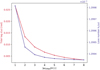 |
Fig. 6 Tidal response of Phobos’ assumed Maxwell rheology. |
7.2 Tidal effects on the dynamics
We now compare the tidal signatures extracted from our coupled propagation results to analytical expectations from the tidal theory (Section 3.2). This aims to demonstrate the realism of our unified model and its ability to accurately reproduce tidal dissipation effects in the system’s dynamics.
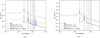 |
Fig. 7 FFT of the differences between the numerical propagated gravity coefficients (coupled model) and the gravity field response predicted by the tidal potential theory (Eqs. (37)–(39)) for the Moon (panel a) and Phobos (panel b). The results are shown here for the ∆S22 variations, but ∆C22 exhibits the same behaviour. The dashed vertical black lines indicate the mean motion frequency and higher harmonics. The orange line represents the FFT obtained when the libration contribution is omitted in the tidal potential (fixing s = 0 in Eqs. (37)–(39)), while the purple line corresponds to the coefficient differences once the libration is accounted for. As a quantitative indication, we also provide the FFT of the propagated coefficients themselves (in green), which was already displayed in Figure 3. Finally, the red dot indicates the contribution of the once-per-orbit libration to the tidal response at the once-per-orbit forcing (showing great agreement with the peak of the gravity differences at this frequency in the no libration case). |
Secular evolution of the satellite’s semi-major axis and eccentricity caused by its own tidal deformation.
7.2.1 Effects of satellite tides on the moon’s orbit
As already highlighted in Section 6.3, tidal dissipation in the satellite causes a secular variation of its own semi-major axis and eccentricity. The secular rates extracted from our propagated orbit for both the Moon and Phobos are reported in Table 2, for the default propagation settings provided in Section 5.3. For the Moon, the orbital evolution caused by satellite tides is in very good agreement with the linear approximations as found in Eqs. (58a) and (59). For Phobos, on the other hand, the non-negligible contribution of the physical libration to the total amount of orbital energy being dissipated should be taken into account. The secular rates of Phobos’ semi-major axis and eccentricity obtained with our coupled model match the libration-augmented linear approximations (Eq. (65)).
The insights brought by this good agreement between the propagation results and the linear approximations in Eqs. (65) are twofold. On one hand, it confirms that Eqs. (58a) and (59), despite being first-order single-frequency linear approximations, accurately describe the main satellite dissipation signatures in the satellite’s own orbit. On the other hand, this successful comparison also validates the ability of our coupled model to produce realistic tidal dissipation effects on the system’s dynamics. This is a crucial validation point, especially given how highly sensitive the orbital migration rate induced by satellite tides is to the consistent modelling of the synchronous satellite’s rotation and tidal response, as highlighted by our discussion in Section 3.6. Following our discussion in Section 3.5, the fact that the da/dt is in agreement with Eq. (58a) rather than Eq. (58b) already suggests that the coupled model accurately reproduces not only the dissipation of orbital energy, but also the contribution of the S 22 offset necessary to maintain the spin-orbit resonance, as will be further discussed in Section 7.2.2.
Our results validate the behaviour of our coupled model for the Moon’s and Phobos’ nominal tidal dissipation settings reported in Table 1. To demonstrate the general applicability of our findings, we ran the coupled propagation for different global relaxation times τ, thus varying the τ/τe ratio and the corresponding equivalent k2/Q. The secular rates of the satellite’s semi-major axis and eccentricity are expected to scale linearly with k2/Q (Eqs. (58a) and (59)), which is indeed what we obtain with our coupled model, as shown in Figure 8. The consistency of our results over different planet–moon systems, one with and one without a notable libration contribution, and different relaxation times provides a robust validation of our coupled propagation.
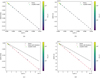 |
Fig. 8 Evolution of the satellite’s orbital elements due to the effect of its own tidal dissipation, for varying relaxation times. Panel a: the Moon’s semi-major axis; panel b: the Moon’s eccentricity; panel c: Phobos’ semi-major axis; panel d: Phobos’ eccentricity. The linear approximations from the tidal theory are given by Eqs. (58a) and (59) for the semi-major axis and eccentricity, respectively, and the contribution of librations is described by Eq. (65). |
7.2.2 Effects of satellite tides on the moon’s rotation
As discussed in Section 6.2, the satellite’s dynamics propagated by our coupled model maintain spin-orbit resonance. This implies that the triaxial and tidal torques acting on the satellite’s rotation cancel out (on average, and neglecting the (very) small deceleration of the satellite’s rotational rate to maintain the resonance with the satellite’s shrinking orbit, Eq. (58a)). To investigate whether this balance is consistent with what tidal theory predicts (Section 3.3), we first computed the secular torque caused by satellite tides. To this end, we computed the torque exerted by the central planet on the time varying part of the satellite’s gravity field, averaged over one orbit. Our results are reported in Table 4 and show very good agreement between the tidal torque evaluated from our propagation results and the one given by the analytical expression in Eq. (45). In Phobos’ case, the contribution of the physical libration, again automatically included in the coupled propagation, is crucial to take into account for the analytical predictions to match the propagation results.
To conserve the spin-orbit resonance despite this residual tidal torque, Section 3.5 highlighted the need for a compensating torque, expected to be provided by a subtle re-orientation of the satellite’s trixial shape (i.e., non-zero (static) S22 gravity coefficient). As reported in Table 3, the static part of S22 extracted from our coupled propagation matches well with the theoretical value expected to ensure the torque balance (Eq. (63)). This result is remarkable in that it automatically follows from the concurrent propagation of the satellite’s orbit, rotation, and tidal deformation, and of the feedback between these different dynamics. It proves that our coupled model consistently accounts for all the dynamical couplings at play, with the satellite’s rotation naturally adapting to the tidal deformation to maintain the resonance.
These results were confirmed over varying relaxation times (i.e., tidal dissipation parameters). The spin-orbit resonance is always conserved: the residual tidal torque and the compensating static S 22 coefficient both linearly scale with k2/Q, as predicted by Eqs. (45) and (63). Figure 9a shows how the static S 22 indeed remains in agreement with theoretical expectations for varying k2/Q. Again, the robustness of our findings irrespective of the amount of tidal dissipation taking place brings extra confidence in our coupled model.
7.3 A note on planet tides
Although this paper focusses on the modelling of the tides raised by the planet on a synchronous satellite, the tides raised by the satellite on its central planet also affect the satellite’s orbit, and more specifically the secular evolution of its semi-major axis and eccentricity (Eqs. (56) and (57), respectively).
Notes. The S22 extracted from our coupled propagation matches the theoretical expectation (Eq. (63)), including the non-negligible contribution of Phobos’ once-per-orbit libration.
Planet tides are less challenging to model than the tides raised on a synchronous satellite: in the absence of the 1:1 com-mensurability between the orbital and rotational periods of the perturbed body, the leading forcing mode ω22000 does not vanish and dominates the tidal response (and its subsequent dynamical effects). Unlike in the case of synchronous satellite tides, the main orbital, rotational, and tidal forcing frequencies differ. This also implies that the very strict requirements in terms of orbit-rotation-tidal deformation modelling consistency for synchronous satellites do not apply to the case of planet tides. Classical decoupled approaches are thus perfectly suitable. Nevertheless, we still tested the ability of our coupled model to reproduce the effects of planet tides on the satellite’s orbit. To this end, we performed a coupled propagation of the orbit, rotational dynamics, and tidal deformation, for both the Earth and Mars.
For the sake of conciseness, and given that planet tides are not the main application focus of our unified model, we only comment on the secular evolution of the satellite’s semi-major axis and eccentricity, and compare the values extracted from our coupled results to tidal theory expectations (Eqs. (56)–(57)). The results of this comparison are reported in Table 5, while the time evolutions of a and e can be found in Appendix E (Figures E.1a–E.1b and E.1c–E.1d f or the Earth and Mars, respectively). The semi-major axis changing rates da/dt are in good agreement with the theoretical values given by Eq. (56), demonstrating the applicability of our unified model to planet tides.
The effects of planet tides on the satellite’s eccentricity, however, are too small to be robustly extracted from our propagation results. The expected secular trends in e due to planet tides as evaluated from Eq. (57) are about 10−13 10−14 smaller than the periodic variations of e shown in Figure−E.1, preventing us from robustly extracting such a small eccentricity secular rate. This limitation, however, is an inherent property of the system’s (perturbed) dynamics, rather than a modelling artifact. The secular change in eccentricity is known to be dominated by satellite tides, the effect of planet tides being comparatively negligible (see Eqs. (57) and (59), being mindful that the perturber/perturbed mass ratio is inverted), and thus harder to isolate from periodic perturbations. This satellite tide-specific signature in the eccentricity is actually exploited to decorre-late planet and satellite dissipation parameters in ephemerides analyses (e.g., Lainey et al. 2009). Our results show that adopting a fully coupled approach does not overcome the numerical limitations encountered when attempting to distinguish such small effects from dynamical noise. Nonetheless, capturing the full forcing frequency spectrum without being limited to linear orbital effects makes the coupled model more likely to be sensitive to possible decorrelations between different signatures, if above detectability level. When fitting real data, satellite and planet dissipation can also be disentangled by combining spacecraft and moon observational constraints (as will be done for Juice and Europa Clipper). Such joint inversions would also greatly benefit from the incorporation of tides in both moon and spacecraft dynamics, which our coupled approach naturally supports.
Averaged torques (in N.m) over an integer number of orbits raised by tides on the Moon and on Phobos.
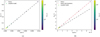 |
Fig. 9 Compensating static S22 values for varying relaxation times for the Moon (panel a) and Phobos (panel b). The value expected from the tidal theory (with and without librations) is computed from Eq. (63). |
Secular evolution of the satellite’s semi-major axis and eccentricity caused by the tides it raises on its central planet.
8 Conclusions
This work focussed on the consistent modelling of tides, orbits, and rotations in planet–synchronous satellite systems. We first provided an overview of relevant tidal dynamics theory (Sections 3.2 and 3.3) to gain insights into the physical realism and applicability of classical modelling strategies, where the orbit, rotation, and tides are typically handled separately (Section 3.4). This specifically shed light onto the unique consistency challenges inherent to the modelling of tides raised on a synchronous satellite (Sections 3.5 and 3.6). To address the shortcomings of classical decoupled models, we proposed a unified propagation of the satellite’s translational and rotational dynamics, concurrently with the numerical integration of its gravity coefficient variations under tidal forcing.
Applying this coupled model to the Earth–Moon and Mars–Phobos systems (see Section 5) demonstrates that it reproduces realistic dynamics and, crucially, that both the satellite’s gravitational response to tides and its feedback on the dynamics are in agreement with the tidal theory. More precisely, the propagated time variations of the satellite’s degree-two gravity coefficients match the analytical expressions derived from the tidal potential (Eqs. (37)–(39), see Section 3.2.2). The remaining differences between the propagated and predicted gravity variations can be attributed to additional librations at harmonics of the orbital frequency which were neglected in Eq. (20), but automatically accounted for in the coupled propagation.
The secular evolutions of the semi-major axis and eccentricity of our propagated orbits due to satellite tides are also aligned with the linear approximations provided in the literature (Eqs. (58a) and (59)). Our results moreover confirm a subtle re-orientation of the satellite’s triaxial shape to generate a restoring trixial torque, exactly compensating for the residual tidal torque. As already investigated in Williams & Efroimsky (2012), among others, this torque balance ensures the conservation of the spin-orbit resonance, thus respecting the exact synchronicity observed for the Solar System’s natural satellites. Finally, for Phobos, the non-negligible enhancement of tidal dissipation effects due to large physical librations also matches theoretical expectations (Frouard & Efroimsky 2017; Efroimsky 2018).
It should be noted that the proposed implementation of the coupled orbit-rotation-tides model still relies on a number of simplifying assumptions which should be revisited to make this framework suitable for high-accuracy applications. This will be critical to fit our coupled model to the actual dynamics of the planet–satellite(s) system under investigation, especially in the context of ephemerides and tidal dissipation parameters estimation. Some of these assumptions only pertain to simplifying the set-up choices that we adopted to facilitate the identification of tidal signatures (more easily detectable in a less perturbed dynamical environment), and therefore the interpretation of our results. Applying our proposed unified approach in a real-case scenario will require moving away from the simplified two-dimensional case we considered. Out-of-plane effects and third-body perturbations should be accounted for, and can be directly incorporated in our equations (see Section 4). Our implementation can also be very easily expanded to include tides raised by multiple bodies. This is an important limitation of Kaula’s tidal potential expansion: it only holds when modelling the tides raised by the central planet on the satellite and vice versa, but cannot be readily applied to satellite–satellite tides for instance. Our coupled model, however, can be expanded to account for multiple tide-raising bodies. It should finally be noted that, when fitting our model to an actual system, difficulties in finding an adequate initial state (see Section 5.2 and Appendix A) are expected to vanish (or at least lessen) as our model will naturally try to reproduce the system’s damped dynamics.
A modelling choice that needs to be properly understood and possibly revisited in future steps is the use of a simple interior model for the tidal response, which assumes a homogenous interior (rather than stratified) and Maxwell rheology (as opposed to more realistic rheological models such as Andrade). Fitting such a model to actual observations of the system’s dynamics is therefore equivalent to finding an effective Maxwell model reproducing the body’s tidal response as best as possible. Whether this Maxwell description can approximate the body’s actual response to yield statistical robust and physically realistic estimates of its interior properties, depending on its internal structure and on the forcing it is subject to, will have to be investigated when progressing towards such estimation-focusses analyses. Adopting a different rheology in our framework would require the derivation of the corresponding  in Eq. (93). Our coupled formulation would remain unchanged except for the incorporation of a different rheology in Eq. (69), which should be translated into a time-domain differential equation for the gravity coefficients, as currently done with the Maxwell model in Section 4.2.
Furthermore, as discussed in Section 5.2.2, the differential equations governing the gravitational deformation (Eqs. (74)–75) do not automatically account for the body’s non-hydrostatic shape. This requires incorporating known deviations from hydrostatic equilibrium as a static field to which the propagated time-varying deformation is added (Eqs. (96)–(97), see Section 5.2.2). Handling this distinction between the body’s static and dynamic response to tides in an estimation, whereas both are influenced by its internal structure and properties, will need to be developed within the current framework.
Nonetheless, our unified dynamical model for modelling of tides in planet–synchronous satellite dynamical systems ensures the fully consistent representation of the feedback between orbit, rotation, and tidal response, intrinsically accounting for all forcing frequencies and all couplings involved. This represents an important improvement compared to present decoupled approaches, which will not be sufficient to meet the challenges of upcoming space missions such as Juice and Europa Clipper (Van Hoolst et al. 2024; Fayolle 2025). In addition to consistency in the satellite’s dynamical evolution, our unified model offers an inherently coherent and robust way to incorporate tidal effects in both the dynamics of the satellite itself, and those of a nearby spacecraft. This is an important modelling aspect for upcoming planetary missions to natural satellites, such as Juice (Van Hoolst et al. 2024; Fayolle 2025), Europa Clipper (Roberts et al. 2023), MMX (Matsumoto et al. 2021), and Hera (Gramigna et al. 2024), and future exploration of icy moons (e.g., UOP, ESA’s L4 mission to Enceladus), where tidal signatures will potentially be detectable from both the spacecraft and moon’s dynamics.
Finally, our extensive review of the modelling of tides and of their effects on the system’s dynamics in Section 3 underlines another limitation of classical models when estimating tidal dissipation parameters from their effects on the moon’s orbit, also discussed in Magnanini et al. (2026). In the moon’s dynamics, the signature of tidal dissipation on the one hand, and that of a small misalignment of the satellite’s triaxial shape with respect to the planet’s direction at periapsis (i.e., non-zero static S 22 coefficient or, equivalently, non-zero longitude at peri- and apoapsis) on the other hand, are nearly identical (both for the translational and rotational dynamics, see details in Section 3.5). In estimation analyses from real data, distinguishing between these two effects is not only extremely challenging (if at all possible) but would only also be physically misleading: they are intrinsically linked manifestations of the satellite’s deformation, and should therefore not be treated in a decoupled manner.
Our coupled model presents us with an elegant way to overcome this difficulty by offering a different fully consistent parametrisation of the problem. The direct incorporation of the satellite’s rheology model in the equations of motion provides us with a natural way to link some of the satellite’s interior properties (rigidity µ, viscosity η) to its complete dynamical response (including the aforementioned re-orientation of its trixial shape). Such an approach circumvents the need for intermediate parameters such as tidal Love numbers k2 to both parametrise the satellite’s tidal response and extract its signature from the moon’s own dynamics or those of a nearby spacecraft. This has the potential to facilitate more direct and robust insights into the physics of the moons’ interiors in future data analyses of planetary missions.
Acknowledgements
S.F. acknowledges support through the European Space Agency (ESA) Research Fellowship Programme in Space Science. The authors would like to thank the anonymous reviewer for their constructive feedback and useful suggestions, which notably improved the clarity and quality of this manuscript.
References
- Bagheri, A., Khan, A., Efroimsky, M., Kruglyakov, M., & Giardini, D. 2021, Nat. Astron, 5, 539 [Google Scholar]
- Borderies, N., & Yoder, C. 1990, A&A, 233, 235 [NASA ADS] [Google Scholar]
- Boué, G. 2017, CM&DA, 128, 261 [Google Scholar]
- Boué, G., & Efroimsky, M. 2019, CM&DA, 131, 1 [Google Scholar]
- Boué, G., Correia, A. C., & Laskar, J. 2016, CM&DA, 126, 31 [Google Scholar]
- Correia, A. C., Boué, G., Laskar, J., & Rodríguez, A. 2014, A&A, 571, A50 [NASA ADS] [CrossRef] [EDP Sciences] [Google Scholar]
- Dirkx, D., Lainey, V., Gurvits, L., & Visser, P. 2016, P&SS, 134, 82 [NASA ADS] [CrossRef] [Google Scholar]
- Dirkx, D., Mooij, E., & Root, B. 2019, Apss, 364, 1 [Google Scholar]
- Dirkx, D., Fayolle, M., Garrett, G., et al. 2022. EPSC2022, (EPSC2022-253). [Google Scholar]
- Dirkx, D., Fayolle, S., Avillez, M., et al. 2025, EPSC, DPS2025, 673 [Google Scholar]
- Durante, D., Hemingway, D., Racioppa, P., Iess, L., & Stevenson, D. 2019, Icarus, 326, 123 [NASA ADS] [CrossRef] [Google Scholar]
- Efroimsky, M. 2012, CM&DA, 112, 283 [Google Scholar]
- Efroimsky, M. 2018, Icarus, 306, 328 [Google Scholar]
- Efroimsky, M., & Lainey, V. 2007, Geophys. Res. Planets, 112, E12 [Google Scholar]
- Efroimsky, M., & Makarov, V. V. 2014, ApJ, 795, 6 [NASA ADS] [CrossRef] [Google Scholar]
- Efroimsky, M., & Williams, J. G. 2009, CM&DA, 104, 257 [Google Scholar]
- Emelyanov, N. 2018, MNRAS, 479, 1278 [Google Scholar]
- Fayolle, M., Dirkx, D., Lainey, V., Gurvits, L., & Visser, P. 2022, P&SS, 219, 105531 [Google Scholar]
- Fayolle, S. 2025, Natural satellites ephemerides: The Galilean moons’ dynamics in the JUICE-Europa Clipper era. Dissertation (TU Delft) [Google Scholar]
- Frouard, J., & Efroimsky, M. 2017, CM&DA, 129, 177 [Google Scholar]
- Fukushima, T. 2008, AJ, 135, 2298 [Google Scholar]
- Goldreich, P., & Gold, T. 1963, MNRAS, 126, 257 [Google Scholar]
- Goldreich, P., & Soter, S. 1966, Icarus, 5, 375 [Google Scholar]
- Goossens, S., van Noort, B., Mateo, A., Mazarico, E., & van der Wal, W. 2024, Nat. Astron, 8, 846 [Google Scholar]
- Gramigna, E., Manghi, R. L., Zannoni, M., et al. 2024, P&SS, 246, 105906 [Google Scholar]
- Grasset, O., Dougherty, M., Coustenis, A., et al. 2013, P&SS, 78, 1 [Google Scholar]
- Henning, W. G., O’Connell, R. J., & Sasselov, D. D. 2009, ApJ, 707, 1000 [Google Scholar]
- Iess, L., Jacobson, R. A., Ducci, M., et al. 2012, Science, 337, 457 [NASA ADS] [CrossRef] [Google Scholar]
- Jacobson, R. A. 2022, AJ, 164, 199 [NASA ADS] [CrossRef] [Google Scholar]
- Kaula, W. M. 1961, Geophys. J. Int., 5, 104 [Google Scholar]
- Kaula, W. M. 1964, Rev. Geophys., 2, 661 [Google Scholar]
- Lainey, V. 2016, CM&DA, 126, 145 [Google Scholar]
- Lainey, V., Duriez, L., & Vienne, A. 2004, A&A, 420, 1171 [NASA ADS] [CrossRef] [EDP Sciences] [Google Scholar]
- Lainey, V., Dehant, V., & Pätzold, M. 2007, A&A, 465, 1075 [NASA ADS] [CrossRef] [EDP Sciences] [Google Scholar]
- Lainey, V., Arlot, J.-E., Karatekin, Ö., & Van Hoolst, T. 2009, Nature, 459, 957 [Google Scholar]
- Lainey, V., Karatekin, Ö., Desmars, J., et al. 2012, ApJ, 752, 14 [Google Scholar]
- Lainey, V., Noyelles, B., Cooper, N., et al. 2019, Icarus, 326, 48 [Google Scholar]
- Lainey, V., Casajus, L. G., Fuller, J., et al. 2020, Nat. Astron., 4, 1053 [Google Scholar]
- Lambeck, K. 1980, Cambridge Monographs on Mechanics and Applied Mathematics (Cambridge: Cambridge University Press) [Google Scholar]
- Lari, G. 2018, CM&DA, 130, 50 [Google Scholar]
- Le Maistre, S., Rosenblatt, P., Rambaux, N., et al. 2013, P&SS, 85, 106 [Google Scholar]
- Lemoine, F. G., Goossens, S., Sabaka, T. J., et al. 2013, Geophys. Res. Planets, 118, 1676 [Google Scholar]
- Levrard, B. 2008, Icarus, 193, 641 [Google Scholar]
- MacDonald, G. J. 1964, Rev. Geophys, 2, 467 [Google Scholar]
- Magnanini, A., Zannoni, M., Casajus, L. G., et al. 2024, A&A, 687, A132 [NASA ADS] [CrossRef] [EDP Sciences] [Google Scholar]
- Magnanini, A., Zannoni, M., & Lainey, V. 2026, A&A, in press., https://doi.org/10.1051/0004-6361/202453210 [NASA ADS] [CrossRef] [EDP Sciences] [Google Scholar]
- Makarov, V. V., & Efroimsky, M. 2013, ApJ, 764, 27 [Google Scholar]
- Malhotra, R. 1991, Icarus, 94, 399 [NASA ADS] [CrossRef] [Google Scholar]
- Martinez, J., Dirkx, D., & Fayolle, S. 2025, A&A, 700, A233 [NASA ADS] [CrossRef] [EDP Sciences] [Google Scholar]
- Matsumoto, K., Hirata, N., Ikeda, H., et al. 2021, EPS, 73, 1 [Google Scholar]
- Mignard, F. 1980, Moon Planets, 23, 185 [NASA ADS] [CrossRef] [Google Scholar]
- Murray, C. D., & Dermott, S. F. 1999, Solar System Dynamics (Cambridge University Press) [Google Scholar]
- Pappalardo, R. T., Buratti, B. J., Korth, H., et al. 2024, Space Sci. Rev, 220, 40 [Google Scholar]
- Park, R., Jacobson, R., Gomez Casajus, L., et al. 2025, Nature, 638, 69 [Google Scholar]
- Peale, S. 1999, Annu. Rev. Astron. Astrophys, 37, 533 [Google Scholar]
- Peale, S. J., & Cassen, P. 1978, Icarus, 36, 245 [NASA ADS] [CrossRef] [Google Scholar]
- Peale, S. J., Cassen, P., & Reynolds, R. T. 1979, Science, 203, 892 [Google Scholar]
- Petit, G., Luzum, B., et al. (2010), IERS conventions. IERS Technical note, 36 [Google Scholar]
- Rambaux, N., Castillo-Rogez, J. C., Williams, J. G., & Karatekin, Ö. 2010, Geophys. Res. Lett, 37, 4 [Google Scholar]
- Rambaux, N., Castillo-Rogez, J., Le Maistre, S., & Rosenblatt, P. 2012, A&A, 548, A14 [NASA ADS] [CrossRef] [EDP Sciences] [Google Scholar]
- Roberts, J. H., McKinnon, W. B., Elder, C. M., et al. 2023, Space Sci. Rev., 219, 46 [Google Scholar]
- Rovira-Navarro, M., Matsuyama, I., & Berne, A. 2024, Planet. Sci. J,, 5, 129 [Google Scholar]
- Tobie, G., Auclair-Desrotour, P., Běhounková, M., et al. 2025, Space Sci. Rev., 221, 1 [Google Scholar]
- Van Hoolst, T., Tobie, G., Vallat, C., et al. 2024, Space Sci. Rev., 220, 54 [Google Scholar]
- Walker, M. E., & Rhoden, A. R. 2022, Planet. Sci. J., 3, 149 [Google Scholar]
- Wigner, E. 1959, Group Theory and Its Application to the Quantum Mechanics of Atomic Spectra (New York: Academic Press) 5 [Google Scholar]
- Williams, J. G., & Boggs, D. H. 2015, Geophys. Res. Planets, 120, 689 [Google Scholar]
- Williams, J. G., & Efroimsky, M. 2012, CM&DA, 114, 387 [Google Scholar]
- Williams, J. G., Konopliv, A. S., Boggs, D. H., et al. 2014, Geophys. Res. Planets, 119, 1546 [Google Scholar]
- Willner, K., Oberst, J., Hussmann, H., et al. 2010, Earth Planet. Sci. Lett., 294, 541 [Google Scholar]
- Wisdom, J. 2008, Icarus, 193, 637 [Google Scholar]
- Yoder, C. F., & Peale, S. J. 1981, Icarus, 47, 1 [CrossRef] [Google Scholar]
In the rest of this work, satellite tides refer to tides raised by the central planet on the satellite, while planet tides designate tides raised by the satellite on the central planet. We moreover restrict ourselves to moon–planet tides.
The rotation of the spherical harmonics coefficients is performed using Wigner D-matrices (Wigner 1959), following the transformation scheme detailed for example in Boué (2017) and Dirkx et al. (2019).
For notation convenience, we choose to directly include the −mθ component into the βlmpq definition, as done for example in Lambeck (1980), but unlike the convention followed in Kaula (1964) or Efroimsky & Williams (2009).
This condition differs from the one proposed in Frouard & Efroimsky (2017), where only q = q′ and s = s′ terms were reported to have a secular contribution. However, secular terms arise for all identical ratios q/s = q′/s′.
For planet tides, k2 and Q here refer to the planet’s tidal parameters, and the asterisk superscript designates the tide-raising satellite.
Conversely, for satellite tides, the ⋆ superscript designates the planet, and the tidal quantities k2 and Q in Eqs. (58a)–(59) refer to the satellite’s.
When performing this derivation starting from the tidal potential expansion (Eq. (30)), one should be mindful that the forcing mode ω22000 no longer vanishes in the case of pseudo-synchronous equilibrium.
A similar derivation with different body-fixed frame convention can for instance be found in Murray & Dermott (1999).
This definition of the so-called gravitational state is specific to our simplified two-dimensional case but could easily be expanded and generalised to describe a three dimensional problem.
 contains the extended component of the perturber’s gravitational potential only.
We purposely use the same gravity field model as the one on which the considered ephemeris solution relied.
Appendix A Finding a good initialisation for the Mars–Phobos dynamical system
Mars and Phobos form a more dynamically complex system than the Earth–Moon case, thus making the obtention of a suitable initial condition more difficult to attain. The relatively close planet–satellite distance, combined with Phobos’ aspheri-cal shape, causes a very strong coupling in Phobos–Mars’ mutual dynamics. The modelling of their entangled dynamics is further complicated by Phobos’ longitudinal normal mode being very close to the moon’s orbital period, and thus to the main once-per-orbit gravitational forcing which drives the evolution of the system’s dynamics. Finding an adequate initial state for Phobos’ numerically integrated gravity coefficients is thus particularly critical. If the initial coefficient values upon initialisation are chosen too far from the values they converge to during the propagation (which are driven by the equilibrium potential, see Eqs. 74–75), the longitudinal normal mode noticeably migrates. The normal mode indeed depends on Phobos’ moments of inertia (Eq. 94), and therefore varies along with its gravity field. This increases the risk of passing the normal mode resonance during the propagation, and significantly complicates the obtention of a damped initial state (see Section 5.2.1).
To circumvent the aforementioned challenges, we artificially set the fluid Love number to a very small value  while still defining the global and Maxwell relaxation times τ and τe such that they match the expected k2 and Q parameters at the main tidal forcing frequency, just as done for the Earth–Moon case. Physically, this is equivalent to considering that the body’s response to the static tide (modelled by the fluid Love number) is already incorporated in Phobos’ static field (Eqs. 98–99), while the propagated gravity field variations include the dynamic tide response. To verify that scaling the fluid Love number kf does not affect Phobos’ tidal response (provided that τ and τe are modified accordingly), Figure A.1 shows the frequency-dependent Love number k2(ωlmpq) and phase lag ϵlmpq for our artificially small fluid Love number kf = 0.01, and for the hydrostatic value kf = 1.5. Both the k2(ωlmpq) and ϵlmpq values are indeed indistinguishable between the two kf cases. This demonstrates that our rheology model can produce a realistic tidal deformation, irrespective of the chosen value for the fluid Love number.
The advantage of (artificially) scaling down kf for the Mars–Phobos case is twofold. First, it eliminates the transient part of the propagation where the gravity coefficients converge to their  -driven equilibrium value. Second, by initialising the propagation using Phobos’ present gravity field solution, we automatically ensure its compatibility with the initial translational-rotational state which we directly extract from Phobos’ current ephemeris.11 We thus guarantee the self-consistency of our state initialisation, an aspect that is far more critical in a highly coupled dynamical system such as the one formed by Mars and Phobos than it is for the Earth–Moon case. Let us moreover recall that the purpose of this work is to investigate whether our unified orbital-rotational-tidal model accurately reproduces the main tidal dissipation and resulting dynamical evolution features, a process in no way hindered by artificially scaling the fluid Love number value.
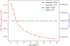 |
Fig. A.1 Tidal response of Phobos’ for kf =0.01 (artificially small) and kf = 1.5 (hydrostatic case). |
Appendix B Results of the damping algorithm
In this Appendix, we briefly present the results of the damping algorithm introduced in Section 5.2.1. Figure B.1a shows the undamped and damped FFTs of Mars’ longitude in the Phobos-fixed reference frame, while Figure B.1b focusses on the FFTs of Phobos’ propagated ∆S22 variations. For the sake of brevity, we here only provide the damping results for the Mars–Phobos case, but the damping algorithm performs similarly for the Earth–Moon system. Furthermore, while only the FFT of the variations in S22 is displayed, identical behaviours are observed when looking at the FFTs of the undamped and damped ∆C20 and ∆C22. As expected, the damping algorithm removes the effect of the normal modes from the satellite’s rotational dynamics (Figure B.1a), thus also successfully preventing these modes from contaminating the propagated gravitational deformation (Figure B.1b). The FFTs of Phobos’ damped rotation and deformation indeed no longer exhibit a peak at the normal mode frequency, but instead only retain the forcings occurring at harmonics of the orbital frequency (in agreement with the tidal potential theory, see Section 3.2). As a final note, the fact that the normal mode forcing initially present in the undamped rotational dynamics spills in the propagated tidal deformation is additional evidence of the strong rotation-tides couplings discussed in Section 3, justifying the need for a coupled modelling approach.
Appendix C Contribution of each forcing mode to the tidal deformation
This Appendix provides more details on the modal decomposition of the tidal response. Table C.1 first lists the leading eccentricity functions G20q(e) together with the corresponding (libration-free) forcing modes ωlmpq for the specific case of tides raised on a synchronous satellite (see Section 3.2, Eq. 27). G200(e) is the only term in O(e0), which therefore identified lmpq = 2200 as the leading forcing mode, provided that ω2200 ≠ 0. As reported in Table C.1 and discussed at length in Section 3.2, this mode vanishes in case of a 1:1 spin-orbit resonance (ω2200=0), leaving lmpq = 220, −1 and lmpq = 2201 as the dominating forcing modes.
For both the Moon and Phobos, Table C.2 then provides the amplitudes |∆C, S2m| of the expected gravity coefficient variations ∆C2m and ∆S2m (the amplitudes are identical for the cosine and sine coefficients), as derived from the tidal potential theory (Eqs. 38–39). The amplitudes of these coefficient variations are separately evaluated for each forcing mode ωlmpqs. We first report the amplitude of the libration-free gravitational deformation (i.e., s = 0) at each forcing mode ωlmpq0. The total contribution of the once-per-orbit libration |∆C, S2m|(ωlmpqs)s≠0 is then also provided (last two columns):
 (C.1)
(C.1)
For Phobos, unlike in the Moon’s case, the non-negligible enhancement of the tidal deformation caused by the (large) once-per-orbit libration is immediately apparent.
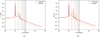 |
Fig. B.1 Damping algorithm results. In both figures, the dashed vertical black lines indicate the mean motion frequency and higher harmonics, while the dashed red line delineates the normal mode frequency. Panel a: Mars’ undamped and damped Phobos-fixed longitude; panel b: Phobos’ undamped and damped ∆S22. |
Appendix D Expansion of the tidal potential to librations with multiple harmonics
As originally developed in Frouard & Efroimsky (2017), the tidal potential expansion given in Eq. 30 can be further expanded to account for multiple libration harmonics (Eq. 20). In particular, we also include a twice-per-orbit harmonic, such that our physical libration model becomes:
 (D.1)
(D.1)
The tidal potential expansions thus requires an additional series expansion (Frouard & Efroimsky 2017):
 (D.2)
(D.2)
Eccentricity functions Glpq(e) for each (libration-free) forcing mode.
The forcing modes  remain identical to those defined in the single-harmonic libration case (Eq. 27):
 (D.3)
(D.3)
Expected tidal mode contributions to ∆C22 and ∆S22
Translating the above potential into time-dependent gravity coefficient variations finally leads to:
 (D.4)
(D.4)
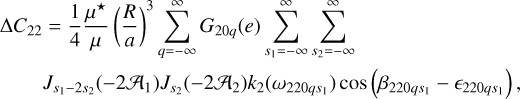 (D.5)
(D.5)
 (D.6)
(D.6)
Appendix E Effects of planet tides on the satellite’s orbit
To support the brief discussion on planet tides effects in Section 7.3 and provide additional context to the numerical results presented in Table 5, Figure E.1 illustrates the results of our coupled model when applied to the modelling of planet tides. More specifically, Figures E.1a–E.1b and E.1c–E.1d show the time evolutions of a and e for the Moon and Phobos, as a result of the tides that they respectively raise on the Earth and Mars.
 |
Fig. E.1 Effects of planet tides on the satellite’s orbit. Panel a: On the Moon’s semi-major axis; panel b: On the Moon’s eccentricity; panel c: On Phobos’ semi-major axis; panel d: On Phobos’ eccentricity. |
All Tables
Secular evolution of the satellite’s semi-major axis and eccentricity caused by its own tidal deformation.
Averaged torques (in N.m) over an integer number of orbits raised by tides on the Moon and on Phobos.
Secular evolution of the satellite’s semi-major axis and eccentricity caused by the tides it raises on its central planet.
All Figures
|
Fig. 1 Schematic representation of the pointing direction of the satellite’s long axis θ and thus of the orientation of the satellite-fixed frame, including the contribution of the longitudinal physical libration γ. The satellite is represented at periapsis (M = 0), at apoapsis (M = π), and at a arbitrarily chosen location along its orbit. In this work, we define the satellite-fixed reference frame such that the satellite’s long axis points towards the planet at apo- and periapsis. |
| In the text | |
|
Fig. 2 Propagated gravity field time variations for the Moon (red) and Phobos (purple) over the entire propagation duration, thus spanning over many orbital periods which here overlay perfectly. |
| In the text | |
|
Fig. 3 Fourier transform of the propagated gravity field coefficient variations (panel a: Moon ; panel b: Phobos). The dashed vertical black lines indicate the mean motion frequency and higher harmonics, while the dashed red line delineates the normal mode frequency. |
| In the text | |
|
Fig. 4 Physical libration extracted from Phobos’ coupled propagation. Panel a: Phobos’ libration as a function of mean anomaly (left y-axis). The red line is directly extracted from the coupled propagation, while the orange dashed line describes the single-frequency libration model (Eqs. (20) and (21)). The purple line (right y-axis) shows the difference between the two, dominated by the twice-per-orbit libration. Panel b: FFT of Phobos’s libration. The dashed vertical black lines indicate the mean motion frequency and higher harmonics, while the dashed red line delineates the normal mode frequency. |
| In the text | |
|
Fig. 5 Secular evolution of the Moon’s semi-major axis (panel a) and eccentricity (panel b) caused by its own tidal deformation. |
| In the text | |
|
Fig. 6 Tidal response of Phobos’ assumed Maxwell rheology. |
| In the text | |
|
Fig. 7 FFT of the differences between the numerical propagated gravity coefficients (coupled model) and the gravity field response predicted by the tidal potential theory (Eqs. (37)–(39)) for the Moon (panel a) and Phobos (panel b). The results are shown here for the ∆S22 variations, but ∆C22 exhibits the same behaviour. The dashed vertical black lines indicate the mean motion frequency and higher harmonics. The orange line represents the FFT obtained when the libration contribution is omitted in the tidal potential (fixing s = 0 in Eqs. (37)–(39)), while the purple line corresponds to the coefficient differences once the libration is accounted for. As a quantitative indication, we also provide the FFT of the propagated coefficients themselves (in green), which was already displayed in Figure 3. Finally, the red dot indicates the contribution of the once-per-orbit libration to the tidal response at the once-per-orbit forcing (showing great agreement with the peak of the gravity differences at this frequency in the no libration case). |
| In the text | |
|
Fig. 8 Evolution of the satellite’s orbital elements due to the effect of its own tidal dissipation, for varying relaxation times. Panel a: the Moon’s semi-major axis; panel b: the Moon’s eccentricity; panel c: Phobos’ semi-major axis; panel d: Phobos’ eccentricity. The linear approximations from the tidal theory are given by Eqs. (58a) and (59) for the semi-major axis and eccentricity, respectively, and the contribution of librations is described by Eq. (65). |
| In the text | |
|
Fig. 9 Compensating static S22 values for varying relaxation times for the Moon (panel a) and Phobos (panel b). The value expected from the tidal theory (with and without librations) is computed from Eq. (63). |
| In the text | |
|
Fig. A.1 Tidal response of Phobos’ for kf =0.01 (artificially small) and kf = 1.5 (hydrostatic case). |
| In the text | |
|
Fig. B.1 Damping algorithm results. In both figures, the dashed vertical black lines indicate the mean motion frequency and higher harmonics, while the dashed red line delineates the normal mode frequency. Panel a: Mars’ undamped and damped Phobos-fixed longitude; panel b: Phobos’ undamped and damped ∆S22. |
| In the text | |
|
Fig. E.1 Effects of planet tides on the satellite’s orbit. Panel a: On the Moon’s semi-major axis; panel b: On the Moon’s eccentricity; panel c: On Phobos’ semi-major axis; panel d: On Phobos’ eccentricity. |
| In the text | |
Current usage metrics show cumulative count of Article Views (full-text article views including HTML views, PDF and ePub downloads, according to the available data) and Abstracts Views on Vision4Press platform.
Data correspond to usage on the plateform after 2015. The current usage metrics is available 48-96 hours after online publication and is updated daily on week days.
Initial download of the metrics may take a while.