| Issue |
A&A
Volume 707, March 2026
|
|
|---|---|---|
| Article Number | A267 | |
| Number of page(s) | 12 | |
| Section | Planets, planetary systems, and small bodies | |
| DOI | https://doi.org/10.1051/0004-6361/202557631 | |
| Published online | 23 March 2026 | |
Longitudinal harmonic components in the Martian upper atmosphere observed by SPICAM and their possible tidal origins
1
State Key Laboratory of Lunar and Planetary Sciences, Macau University of Science and Technology,
Macau,
China
2
Department of Earth and Space Sciences, Southern University of Science and Technology,
Shenzhen,
China
3
LATMOS/IPSL,
Guyancourt,
France
4
LMD/IPSL, Sorbonne Université, PSL Research Université, École Normale Supérieure, École Polytechnique, CNRS,
Paris,
France
★ Corresponding author: This email address is being protected from spambots. You need JavaScript enabled to view it.
Received:
10
October
2025
Accepted:
29
January
2026
Abstract
Context. The longitudinal variations of temperature and pressure in the upper atmosphere of Mars provide important observational constraints on atmospheric waves, including thermal tides.
Aims. This study aims to characterize the longitudinal harmonic components associated with non-migrating thermal tides between 80 and 130 km and to examine their dominant tidal contributions.
Methods. We analyzed nightside temperature and pressure profiles obtained by the Spectroscopy for the Investigation of the Characteristics of the Atmosphere of Mars (SPICAM) instrument on board Mars Express during Mars years 26–30, excluding the global dust storm period. We used simulations from the Mars Planetary Climate Model (PCM) to interpret the observed longitudinal structures.
Results. Wave-2 and wave-3 are the dominant longitudinal components in the SPICAM observations. In contrast, wave-1 is generally weak and its longitudinal variability is consistent with that in the PCM, including the diurnal zonal-mean tide (D0), the stationary planetary wave with zonal wavenumber 1 (SPW1), and the westward propagating semidiurnal tide with zonal wavenumber 1 (SW1). Above 110 km, we also identify a robust wave-4 component. The mode decomposition further indicates that wave-2 and wave-3 are primarily associated with the eastward-propagating diurnal tide with zonal wavenumber 1 (DE1) and the eastward-propagating semidiurnal tide with zonal wavenumber 2 (DE2), respectively. Wave-4 mainly arises from contributions of the eastward-propagating diurnal tide with zonal wavenumber 3 (DE3) and the eastward-propagating semidiurnal tide with zonal wavenumber 2 (SE2).
Conclusions. These results provide new observational constraints on non-migrating thermal tides in the Martian upper atmosphere and show that higher-order longitudinal components, such as wave-4, become increasingly important above 110 km, particularly during dusty seasons. The combined observational and model-based analysis highlights both the robustness of the dominant tidal structures and the limitations of current models in capturing the full complexity of longitudinal variability in the upper atmosphere.
Key words: waves / planets and satellites: terrestrial planets
© The Authors 2026
 Open Access article, published by EDP Sciences, under the terms of the Creative Commons Attribution License (https://creativecommons.org/licenses/by/4.0), which permits unrestricted use, distribution, and reproduction in any medium, provided the original work is properly cited.
This article is published in open access under the Subscribe to Open model. This email address is being protected from spambots. You need JavaScript enabled to view it. to support open access publication.
1 Introduction
The longitudinal variations in temperature and pressure are a prominent feature of the Martian middle and upper atmosphere and reflect the combined influence of thermal tides, planetary waves, and background circulation (e.g., Forbes et al. 2002; Liu et al. 2017). Among these processes, non-migrating thermal tides significantly shape the longitudinal structures of temperature, pressure, density, and winds in the Martian middle and upper atmosphere (e.g., Forbes et al. 2020; Withers et al. 2011). Non-migrating tides are planetary-scale harmonic oscillations that are asynchronous with the apparent motion of the Sun and typically arise from stationary sources such as topography, surface heating, and dust activity (e.g., Jain et al. 2023; Moudden & Forbes 2008a; Wilson 2002).
The longitudinal variations in atmospheric temperatures and pressures associated with non-migrating tides are commonly examined in a local-time–fixed reference frame, in which migrating tidal components remain present but exhibit no longitudinal dependence, contributing only to the zonally symmetric component. In this framework, the remaining longitudinal structures are conveniently described using zonal harmonic components, characterized by their zonal wavenumber (m), and referred to as wave-m components. In particular, the wave-1 to wave-3 components have been widely investigated through observations and modeling (e.g., Forbes et al. 2021; Forbes & Hagan 2000; Gröller et al. 2018; Moudden & Forbes 2008a; Wang et al. 2006; Withers et al. 2011), but the wave-1 component is generally weaker than wave-2 and wave-3 (e.g., Withers et al. 2003, 2011).
To facilitate discussion of the possible wave and tidal origins of the observed longitudinal harmonic components, we adopt a standard tidal notation following previous studies. We denote westward- and eastward-propagating diurnal tides (n = 1; see Equation (1)) with zonal wavenumber s as DWs and DEs, respectively. For semidiurnal (n = 2), terdiurnal (n = 3), and quarterdiurnal (n = 4) oscillations, we use the prefixes S, T, and Q in place of D. We denote zonally symmetric oscillations (s = 0; see Equation (1)) as D0, S0, T0, and Q0. In addition, SPWs denotes a stationary planetary wave with zonal wavenumber s, which is distinct from tidal components. In the present study, we focus primarily on solar tides with periods of one to four sols (n = 1–4), which may contribute to the longitudinal variability of temperatures and pressures in the Martian middle and upper atmosphere. Nevertheless, modeling studies indicate that D0 and SPW1 may contribute significantly to wave-1 (e.g., Forbes & Zhang 2018; Moudden & Forbes 2008b). Overall, observations consistently show that wave-2 and wave-3 dominate the longitudinal variability in the upper atmosphere of Mars (e.g., Banfield et al. 2003; Bougher et al. 2001; Thaller et al. 2020). For example, Gröller et al. (2018) report perturbations dominated by zonal wavenumbers 2 and 3 with amplitudes exceeding 45%. Keating et al. (1998) detected 20% wave-2 density perturbations in the lower thermosphere, while England et al. (2016) report up to 50% wave-2 variability at northern low latitudes. Wave-3 has also been identified in multiple datasets, with temperature perturbations >15 K (Withers & Catling 2010) and CO density variations of 13% between 150 and 185 km (e.g., England et al. 2019; Medvedev et al. 2016). Model simulations have identified the most significant non-migrating tides underlying these wave-2 and wave-3 signatures and indicate that DE1, DE2, and SE1 are the most common tides (e.g., Forbes et al. 2002; Forbes & Hagan 2000; Forbes et al. 2020, 2025).
Recent observational studies have increasingly recognized the importance of wave-4. Liu et al. (2024) provided the first clear detection of wave-4 in density profiles between 150– 200 km, with amplitude peaks near the longitude of 320◦ E, suggesting a robust structure related to dust storms. Jain et al. (2023) report dominant wave-4 components in temperature fields near 170–190 km during Martian years (MYs) 33 and 35, with amplitudes reaching 4.2 K and 2.8 K, respectively. Forbes et al. (2020) combined observations with simulations and show that most wave-4 structures observed between 105 and 115 km within ±55◦ latitude can be attributed to a combination of DE3 and SE2 tides. However, wave-4 structures evolve with altitude, latitude, and season between 80–130 km remains poorly understood.
To better understand the atmospheric environment relevant to Mars entry, descent, and landing (EDL), this study characterizes the seasonal, latitudinal, and vertical variations of longitudinal harmonic components in measured temperatures and pressures between 80 and 130 km. We infer that these components are associated with combinations of non-migrating thermal tides and SPWs sharing the same zonal wavenumber, based on comparisons with Mars Planetary Climate Model (PCM) simulations and previous studies. The present analysis is based on the nighttime temperature and pressure profiles from the Spectroscopy for Investigation of Characteristics of the Atmosphere of Mars (SPICAM) and simulations from the PCM. We confirm for the first time the existence of a significant wave-4 component in this altitude range, and PCM mode decomposition further elucidates the primary tidal sources underlying these non-migrating structures. Section 2 describes their relevant information. We describe corresponding results regarding the structure of the fit non-migrating tides in Section 3, followed by the discussion and conclusions in Section 4.
2 Data and methodology
2.1 Instrument and observations
The SPICAM instrument on board Mars Express (MEX) is a UV spectrometer designed to observe stellar occultations (Bertaux et al. 2006). Retrievals from these spectra provide vertical profiles of atmospheric pressure, density, and temperature (Quémerais et al. 2006), providing an ideal dataset to investigate waves in the middle and upper atmospheres of Mars. We derived longitudinal harmonic components of atmospheric temperatures and pressures between 80–130 km from nightside vertical profiles, and we interpreted their possible associations with non-migrating thermal tides based on PCM simulations and previous studies. To improve statistics, we binned the data by latitude (<30◦), longitude, local solar time (<3 hr), and 30◦ intervals in solar longitude (Ls) for MYs 26–30, excluding data obtained during the global dust storm period in MY 28 (Ls = 265◦–310◦) to ensure nominal conditions (Wolkenberg et al. 2020). The resulting dataset contains 1408 profiles that span 5 MYs, as previous studies have reported that salient structural features of tides are generally repeatable from year to year (Moudden & Forbes 2015; Wu et al. 2015). This dataset substantially extends the analysis of Withers et al. (2011) and is illustrated in Figures 1a–1b. We selected four representative cases – South-Low-Clear, South-Mid-Clear, South-Low-Dusty, and North-Low-Dusty – based on latitude, local time, and season to extract longitudinal harmonic components. “Low” and “Mid” denote latitude bands, while “Clear” and “Dusty” indicate non-dusty and dusty seasons, respectively. Figures 1c–1f (also in Appendix A) show their spatial distributions. This sampling approach enables a more focused comparison of seasonal and latitudinal variability of longitudinal harmonic structures.
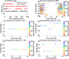 |
Fig. 1 SPICAM data coverage used in this study. (a) Coverage in MYs for all available profiles. (b–f) Data coverage in local time, latitude, and solar longitude for (b) all profiles, (c) South-Low-Clear, (d) South-Mid-Clear, (e) South-Low-Dusty, and (f) North-Low-Dusty cases. The number of profiles is indicated by N. |
2.2 Mars PCM
The Mars PCM serves as a benchmark for our current understanding of Martian atmospheric conditions. It is widely used to simulate Martian atmospheric dynamics from the surface to the upper atmosphere (see Appendix B). Unlike observational data, model simulations provide continuous coverage, which facilitates the analysis of thermal tide wave properties. We used PCM version 5 for our model-observation comparison. The simulations have a horizontal resolution of 5.625◦ × 3.75◦ and 49 vertical levels extending up to 240 km (Angelats i Coll et al. 2005), using the “Climatology” dust scenario (Forget et al. 2009; Montabone et al. 2015, 2020). This dust scenario averages MY24-MY31 dust scenarios, excluding MY25 and MY28 global dust storms (Montabone et al. 2015, 2020). We used two complementary PCM datasets. First, we sampled PCM outputs at the same locations and local times as the SPICAM observations to reproduce the observational sampling. We applied harmonic fitting to this sampled PCM dataset to enable a direct and consistent comparison with the SPICAM measurements. Second, we used the full PCM dataset, which provides complete longitudinal coverage, to investigate the intrinsic contributions of wave modes. The longitudinal harmonic fits for waves 1–4 derived from the full PCM fields are presented in Appendix B (Figures B.1 and B.2).
2.3 Wave fitting mode
Following previous studies, we decomposed the longitudinal variation of a given input, temperature, or pressure by assuming a linear combination of harmonic functions within latitude bins at each altitude level (e.g., Fan et al. 2022; Forbes et al. 2002; Wu et al. 2017). Therefore, for a given input variable X,
![Mathematical equation: $\displaylines{\chi \left( {\lambda ,\phi ,z,{t_{{\rm{LT}}}}} \right) = \sum\limits_{\sigma ,s} {[{C_{\sigma ,s}}\left( {\phi ,z} \right)\cos \left( {\left( {s - \sigma } \right)\lambda + \sigma {t_{{\rm{LT}}}}} \right)} \cr + {S_{\sigma ,s}}\left( {\phi ,z} \right)\sin \left( {\left( {s - \sigma } \right)\lambda + \sigma {t_{{\rm{LT}}}}} \right)] \cr} $](/articles/aa/full_html/2026/03/aa57631-25/aa57631-25-eq1.png) (1)
(1)
where X denotes an observed atmospheric parameter (e.g., temperature or pressure); λ, ϕ, and z represent longitude, latitude, and altitude, respectively (all analyses use altitude coordinates); tLT is the local time; s and σ are the zonal wavenumber and temporal frequency, respectively; and C and S are the harmonic coefficients. Thus, |s − σ| gives the longitudinal wavenumber in a local-time frame, where positive s/σ indicates westward-propagating tides. For example, (s, σ) = (1, 1) corresponds to the diurnal westward wave with wavenumber one. We truncated the expansion at |s − σ| = {0, 1, 2, 3, 4}, retaining only the top five contributing modes and neglecting higher-order terms. Because individual measurement uncertainties are not commensurate with the sol-to-sol variability below 150 km, we used the mean square error between measurements and model predictions as a proxy for the fit uncertainty (Withers 2003). The 1σ values refer to a single composite fit. We derived amplitudes (A) and phases (θ) from the fit coefficients, where
 (2)
(2)
 (3)
(3)
To compare different atmospheric parameters, we used normalized wave amplitudes, defined as fractional deviations from their respective zonal means. Because we derived the longitudinal harmonic components solely from zonal wavenumber decomposition, they represent the total longitudinal variability and do not uniquely correspond to thermal tides or stationary planetary waves based on longitudinal structure alone.
3 Results
To characterize the wave structure, we fit temperature and pressure data for waves 1–4 using Equation (1) (Section 2.3) in 10 km bins between 80 and 130 km. Both SPICAM and sampled PCM fits reveal strong, altitude-dependent seasonal and longitudinal variations. In dusty seasons, SPICAM temperatures are 20–40 K warmer below 110 km and up to 50 K cooler at 130 km than in non-dusty cases. The sampled PCM data capture the corresponding temperature contrasts, although simulations are on average 12 K cooler than 120 km in the non-dusty seasons and 28 K warmer than 110 km in the dusty seasons (Figures 2a–2h). For SPICAM pressures, values in dusty seasons systematically exceed those in non-dusty seasons (Figures 3a–3d). The sampled PCM data reproduce this pattern (Figures 3e–3h), although the amplitudes are generally larger than those observed.
To investigate the longitudinal structure of atmospheric variability in the middle and upper atmosphere, we derived amplitudes and phases of the longitudinal wave components using Equation (1) (Section 2.3). We analyzed these components in terms of their seasonal, latitudinal, and vertical characteristics, and discuss their possible tidal and SPWs contributions below.
3.1 Wave-1
Wave-1 is a weak component in the longitudinal structure, exhibiting small amplitudes and marked seasonal–latitudinal variability. In the observations, wave-1 amplitudes are generally weak (<10%) in both temperature and pressure, with localized enhancements in South-Low-Dusty (19.6% at 115 km in temperature but <10% in pressure; Figures 2k, 3l) and South-Mid-Clear (15% above 110 km in temperature; Figure 2j), and a pressure maximum of 28.8% at 130 km in South-Low-Clear (Figure 3i).
In the sampled PCM data, wave-1 remains the smallest component (≤ 5% in temperature and <10% in pressure; Figs. 2e–2h and 3e–3h). Despite this qualitative similarity in overall weakness, the model-observation consistency for wave-1 remains limited. The sampled PCM phases are systematically shifted eastward by ∼60–120◦, with the best agreement in the South-Low-Clear case and substantially larger discrepancies in the other cases (Figs. 2m–2p and 3m–3p). We quantitatively confirmed this behavior using a coverage-weighted Nσ-based statistical assessment that evaluates the level of agreement between the sampled PCM simulations and the SPICAM observations (Appendix C). The Nσ statistics consistently identify wave-1 as the least consistent component among all longitudinal harmonics, showing comparatively low agreement scores and reduced phase coherence, particularly in the upper altitude bin (80– 110 km) (Tables C.1 and C.2). Given the mixed tidal-planetary wave nature of the extracted longitudinal harmonic components, we used the Nσ-based analysis (Appendix C) to quantify model–observation consistency in terms of longitudinal structure, rather than to attribute individual components to specific physical sources.
Mode decomposition of the full PCM data (Figs. 4a–4h) suggests that the observed wave-1 variability arises primarily from a combination of D0, SPW1, and SW1 components. Individually, these modes are typically weak (≤2–5%), but their contributions increase with altitude, particularly in South-Low-Clear (SPW1 reaching 5.7%; Fig. 4e) and South-Low-Dusty (D0 up to 6.3%; Fig. 4g). The increasing influence of multiple weak and competing components, combined with larger observational uncertainties at higher altitudes, likely reduces the model–observation agreement for wave-1, as quantified by the Nσ-based statistics in Appendix C.
3.2 Wave-2
Wave-2 is a major component of the longitudinal structure and is dominated by DE1 in the PCM data, with strong altitude and seasonal dependence. In SPICAM observations, wave-2 amplitudes increase in South-Low-Clear (20.1% at 130 km in temperature, 31.7% at 130 km in pressure; Figures 2i and 3i) and North-Low-Dusty (18.8% at 95 km in temperature, 26.6% at 100 km in pressure; Figures 2l and 3l). In contrast, both temperature and pressure remain below 10% in South-Low-Dusty (Figures 2k and 3k), consistent with weakening during a major dust storm near Ls = 130◦ (Forget et al. 2009; Smith et al. 2006).
In sampled PCM data, wave-2 amplitudes are generally weak, staying within 5% in temperature, except for North-Low-Dusty (8.2% at 125 km; Figure 2l). The pressure peaks at 17% in South-Low-Clear (100 km; Figure 3i) and 16.8% in North-Low-Dusty (100 km; Figure 3l), while all other cases below 10%. The modeled phases are shifted eastward by 30–90◦, with South-Mid-Clear and North-Low-Dusty showing the largest deviations (Figures 2m–2p and 3m–3p).
Despite these amplitude and phase discrepancies, the overall behavior of wave-2 is strongly case-dependent. The coverage-weighted Nσ statistics show substantially higher agreement scores for wave-2 under dusty conditions than under clear conditions, particularly in the 80–110 km altitude range. In contrast, several clear-season cases exhibit reduced agreement, primarily due to lower phase consistency, especially at higher altitudes (Tables C.1 and C.2).
Mode decomposition identifies DE1 as the primary contributor. In South-Low-Clear, DE1 exhibits a phase reversal (Figures 2m and 4a) and peaks at 18.7% in pressure (Figure 4e). In North-Low-Dusty, DE1+S0 shows steady propagation (Figures 2p and 4d), with DE1 reaching 11% (Figure 4h). In contrast, the other cases show considerably weaker contributions, remaining below 10% in pressure and ≤3% in temperature (Figures 4b and 4g).
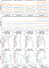 |
Fig. 2 Longitudinal structures of SPICAM temperature observations for (a) South-Low-Clear, (b) South-Mid-Clear, (c) South-Low-Dusty, and (d) North-Low-Dusty. Panels (e)–(h) show the corresponding structures from sampled PCM data. Dots indicate data points and shaded regions represent ±1σ uncertainties of the composite fits. Panels (i) to (l) show the amplitudes and ±1σ uncertainties of waves 1–4, normalized by the zonal mean for the four cases in (a)–(d). For clarity, the SPICAM and sampled PCM profiles are vertically offset by +1 km and −1 km, respectively. The SPICAM amplitudes use dashed semi-transparent lines; PCM amplitudes use solid, opaque lines. Panels (m)–(p) show the corresponding phases and ±1σ uncertainties, defined as the longitude of the first eastward peak from 0◦ for each harmonic component. The temperature structures in the first two rows are vertically offset by [−100, −30, 30, 120, 200, 290] K for 80–130 km altitudes, except for the North-Low-Dusty case, which uses [−100, −30, 70, 210, 320, 450] K. |
3.3 Wave-3
Wave-3 is another major component of the longitudinal structure and is dominated in the PCM by a single DE2 component that propagates steadily upward and exhibits pronounced latitudinal and seasonal dependence. In SPICAM observations, wave-3 amplitudes increase in both temperature and pressure, peaking at 13.2–16.2% at 130 km in dusty-season cases (Figures 2k and 2l). In non-dusty cases, amplitudes remain below 10% in South-Mid-Clear (Figure 2j) but reach 22.5% at 120 km in South-Low-Clear (Figure 2i). For pressure, all cases exceed 20% and show few phase reversals (Figures 3i–3p), indicating a robust and coherent longitudinal structure.
In sampled PCM data, wave-3 amplitudes are weak in temperature (≤6%, with South-Low-Dusty within 5%; Figure 2k) and generally below 15% in pressure, except in South-Low-Clear, where they peak at 37.5% at 130 km (Figure 3i). The simulations are shifted 30–60◦ eastward and show a greater scatter and weaker vertical coherence than the observations (Figures 2m–2p and 3m–3p).
Despite differences in absolute amplitude and phase, the relative longitudinal structure of wave-3 is well reproduced in most cases. The coverage-weighted Nσ statistics indicate consistently high agreement scores for wave-3 in both pressure and temperature, particularly in the 80–110 km altitude range, making it one of the most robustly reproduced longitudinal components among all harmonics (Tables C.1 and C.2).
Mode decomposition of the full PCM identifies DE2 as the dominant contributor to wave-3 variability. In South-Low-Clear, DE2 reaches 3.9% in temperature at 105 km (Fig. 4a) and 21% in pressure at 130 km (Fig. 4e). In both dusty-season cases, DE2 amplitudes exceed 10% (Figs. 4g and h), whereas South-Mid-Clear exhibits an unusually weak DE2 signal of approximately 3% (Fig. 4f). The strong dominance of a single tidal mode and the limited interference from competing components likely contribute to the consistently high agreement scores for wave-3, particularly below 110 km (Tables C.1 and C.2).
3.4 Wave-4
Wave-4 becomes detectable primarily above 110 km in both temperature and pressure. Residual diagnostics, obtained after removing wave-1 to wave-3 components that were fit to the data, together with projections onto the [0◦, 90◦] basis, reveal a characteristic single peak-trough longitudinal structure. SPI-CAM observations in all four cases reveal a coherent wave-4 signal accompanied by a systematic reduction in residual variance (Appendix D; Fig. D.1). The strongest signal occurs in South-Mid-Clear temperature at 95 km (40◦/80◦; Figure 5)b. South-Low-Clear pressure at 120 km shows a distinct pattern (80◦/30◦; Figure 5a). South-Low-Dusty shows a broader uncertainty at 80 km (50◦/10◦; Figure 5c). North-Low-Dusty retains a weak but recognizable signal at 130 km (70◦/25◦; Figure 5d).
In general, wave-4 is a weak component whose amplitudes increase with altitude and become strongest above 110 km, particularly during dusty seasons. The dominant modes in the PCM data are DE3 and SE2. In the observations, wave-4 amplitudes increase mainly above 120 km, peaking in temperature at 18.3% in South-Low-Clear (Figure 2i) and 12.4% in North-Low-Dusty (Figure 2l), while remaining ≤10% in South-Mid-Clear and South-Low-Dusty (Figures 2j and 2k). For pressure, enhancements are confined to South-Low-Clear (16.5% at 125 km) and North-Low-Dusty (10.2% at 100 km; Figures 3i and 3l), while other cases remain below 10% (Figures 3j and 3k).
In sampled PCM data, wave-4 amplitudes remain generally weak in temperature (<5%), with a modest enhancement in South-Low-Dusty (7% at 90 km; Figure 2k). In pressure, they exceed 10% only in South-Low-Clear (13.9% at 130 km) and in dusty cases (Figures 3k, 3l), while remaining <5% in South-Mid-Clear. The modeled phases exhibit persistent eastward shifts of approximately 30–90◦, together with reduced vertical continuity compared with the observations (Figures 2m–2p and 3m–3p).
Despite its relatively small amplitudes, the coverage-weighted Nσ statistics support the presence and vertical evolution of wave-4. Wave-4 maintains moderate to high agreement scores below 110 km, particularly in pressure, whereas reduced phase coherence and increasing uncertainties at higher altitudes contribute to a gradual degradation of agreement (Tables C.1 and C.2). This behavior supports the interpretation of wave-4 as a higher-order longitudinal component that remains physically meaningful but becomes increasingly sensitive to background conditions in the upper thermosphere.
The mode decomposition of the full PCM data indicates that the wave-4 variability is primarily associated with the DE3 and SE2 components. During dusty seasons, DE3 reaches 3.4% in North-Low-Dusty and SE2 reaches 1.9% in South-Low-Dusty (Figs. 4c and 4g). In the non-dusty South-Low-Clear case, DE3 remains the dominant contributor (2.8%), whereas South-Mid-Clear does not show a clearly identifiable tidal signal (Figs. 4a–4d). In pressures, DE3 and SE2 exceed 5% only in South-Low-Clear and South-Low-Dusty (Figs. 4e and 4g), with negligible contributions in the other cases. This sparse and intermittent modal structure is consistent with the weaker and less coherent nature of wave-4 inferred from the coverage-weighted agreement statistics.
Taken together, the four longitudinal harmonics exhibit distinct levels of robustness, vertical coherence, and model– observation consistency. Wave-1 is the weakest and least reproducible component. It is characterized by small amplitudes, strong case dependence, and pronounced phase discrepancies, particularly above 110 km, where competing tidal and planetary-wave contributions and increasing uncertainties reduce agreement. Wave-2 constitutes a major dynamical component, but its amplitudes and phases are strongly modulated by seasonal and dust conditions. This modulation produces pronounced contrasts between dusty and clear cases and reduces consistency under non-dusty conditions. In contrast, wave-3 is the most robust and consistently reproduced harmonic. It is dominated by a single DE2 component with strong vertical coherence, limited modal interference, and consistently high Nσ agreement scores across most cases, especially below 110 km. Wave-4 appears as a higher-order residual component that becomes detectable mainly at higher altitudes. Its amplitudes increase above 110 km, but reduced phase coherence and enhanced sensitivity to background conditions lead to moderate agreement at lower altitudes and progressive degradation aloft. Overall, these results indicate that the reliability of longitudinal harmonics is closely linked to modal simplicity and vertical coherence. Wave-3 provides the most stable diagnostic of large-scale tidal structure, whereas wave-1, wave-2, and wave-4 reflect increasingly complex interactions among tides, planetary waves, and background variability in the Martian upper atmosphere.
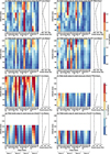 |
Fig. 4 Amplitudes of temperature for different fit tidal modes and the zonal mean derived from the full PCM data for four cases: (a) South-Low-Clear, (b) South-Mid-Clear, (c) South-Low-Dusty, and (d) North-Low-Dusty. Panels (e)–(h) are similar to (a)–(d), but for the pressure field. The mode decomposition includes both tidal components and SPW contributions with the same zonal wavenumber. |
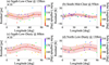 |
Fig. 5 Wave-4 fit based on residuals obtained after subtracting the fit wave-1 to wave-3 components from SPICAM temperature and pressure observations for four cases: (a) South-Low-Clear, (b) South-Mid-Clear, (c) South-Low-Dusty, and (d) North-Low-Dusty. Dots and shaded regions represent the data points and ±1σ uncertainties, respectively. This residual-based analysis verifies that the wave-4 signal identified in the full harmonic fit is not an artifact of noise. |
4 Discussion and conclusions
Nighttime temperature and pressure profiles from SPICAM (MY 26–30, excluding the global dust storm) and PCM simulations using the “Climatology” dust scenario provide the basis for analyzing the longitudinal structure and modal characteristics of longitudinal harmonic components in the Martian upper atmosphere between 80 and 130 km. We interpret these components in the context of non-migrating thermal tides and SPWs. Extending the SPICAM dataset and applying a consistent harmonic fitting framework reveals a robust wave-4 component within this altitude range. This component is most evident above 110 km and exhibits increasing amplitudes toward 130 km, particularly during dusty seasons. We further examined the consistency of the fits through comparisons with PCM simulations. Below 110 km, the simulated and observed longitudinal harmonic components show comparable magnitudes, especially where the fit amplitudes remain small. This comparison evaluates the overall longitudinal structure rather than providing a statistical validation of individual non-migrating tidal amplitudes. A quantitative evaluation explicitly accounting for uncertainties using an Nσ-based metric is presented in Appendix C. Mode decomposition identifies D0, SPW1, and SW1 as the major contributors to wave-1, DE1 and DE2 are dominant for wave-2 and wave-3, and wave-4 is mainly composed of DE3 and SE2.
The fit amplitudes of waves 1–3 fall within the ranges reported by Withers et al. (2011). The North-Low-Dusty case also agrees with Lo et al. (2015), who found amplitudes of ∼10% for wave-1 to wave-3 near 30◦N at 130 km, using daytime CO2 density data under similar sampling conditions. For PCM simulations, wave-2 and wave-3 are the primary contributors, consistent with previous studies (England et al. 2016, 2019; Forbes 2004; Wang et al. 2006). Below 110 km, simulations generally reproduce the amplitudes of statistically significant longitudinal wave components. At higher altitudes, however, increasing divergence among individual wavenumbers – most notably between the weak, mixed wave-1 component and the more coherent higher-order components – reduces the mean agreement. Our findings agree with Kumar et al. (2022), who report that upward propagation of non-migrating tides and better model performance at lower altitudes (60–90 km) compared with higher altitudes (140–165 km). Previous studies show that wave-2 and wave-3 are strongly influenced by topographic forcing (Medvedev et al. 2016; Wilson 2000). In this study, wave-3 exhibits consistently high agreement across most cases (particularly 110 km), while wave-2 shows higher agreement under dusty conditions but greater variability across cases and altitudes.
Modal decomposition of the full PCM shows that wave-2 and wave-3 are dominated by DE1 and DE2, respectively, consistent with previous studies England et al. (2016) Schneider et al. (2020), Kumar et al. (2022). Wave-4 amplitudes remain small below 110 km but increase above this altitude, especially during dusty seasons. This may explain why Withers et al. (2011) excluded this component from their analysis. Wave-4 exhibits vertically coherent structures and eastward phase tilts (Figure 4). In most cases, wave-4 is mainly composed of DE3 and SE2, consistent with Forbes et al. (2020).
Finally, discrepancies between the observations and the PCM simulations, particularly above 120 km, reflect increasing uncertainties in the fit longitudinal harmonic components. These uncertainties, quantified using the mean square error of the fits (Section 2.3), reflect both retrieval-related errors and enhanced sol-to-sol geophysical variability at these altitudes. The temperature, derived by downward integration from the top of the profile and dependent on an assumed upper boundary temperature, carries large uncertainties at high altitudes (Forget et al. 2009). Using a fixed solar flux in simulations may also influence tidal fits in this region. In addition, sparse data coverage during dusty seasons after Ls = 210◦, together with the absence of reliable high-altitude pressure fits, constrains assessment of seasonal evolution and limits detailed interpretation. Addressing these issues requires improved local time, latitudinal, and seasonal sampling, which could be achieved through combined observations from current missions and future instruments with enhanced temporal and spatial coverage.
Data availability
The SPICAM/MEX stellar occultation data are publicly available from the NASA Planetary Data System (PDS) at https://pds-geosciences.wustl.edu/missions/mars_express/spicam.htm. The Mars PCM version 5 and related software are publicly available at https: //svn.lmd.jussieu.fr/Planeto/trunk/LMDZ.MARS (Forget et al. 1999).
Acknowledgements
This research is funded by grants from the Key Technology Research Project of TW-3 (grant no. TW3006) and the FDCT of Macau (grant No. 0013/2023/RIA1 and 0010/2023/AFJ). S.F. acknowledges funding from the National Natural Science Foundation of China through grant No. 42475133, and the Stable Support Plan Program for the Higher Education Institutions of the Shenzhen Science and Technology Innovation Commission through grant No. 20231115103030002. We would also like to thank Dr. Dmitrij Titov for his assistance with the data and Dr. Lori Neary for her valuable support throughout the writing process.
References
- Angelats i Coll, M., Forget, F., López-Valverde, M., & González-Galindo, F. 2005, Geophys. Res. Lett., 32 [Google Scholar]
- Banfield, D., Conrath, B., Smith, M., Christensen, P., & Wilson, R. J. 2003, Icarus, 161, 319 [Google Scholar]
- Bertaux, J.-L., Korablev, O., Perrier, S., et al. 2006, J. Geophys. Res. Planets, 111 [Google Scholar]
- Bougher, S. W., Engel, S., Hinson, D. P., & Forbes, J. M. 2001, Geophys. Res. Lett., 28, 3091 [Google Scholar]
- England, S. L., Liu, G., Withers, P., et al. 2016, J. Geophys. Res. Planets, 121, 594 [Google Scholar]
- England, S. L., Liu, G., Kumar, A., et al. 2019, J. Geophys. Res. Space Phys., 124, 2943 [Google Scholar]
- Fan, S., Guerlet, S., Forget, F., et al. 2022, Geophys. Res. Lett., 49, e2021GL097130 [Google Scholar]
- Forbes, J. M. 2004, Adv. Space Res., 33, 125 [Google Scholar]
- Forbes, J. M., & Hagan, M. E. 2000, Geophys. Res. Lett., 27, 3563 [Google Scholar]
- Forbes, J. M., & Zhang, X. 2018, J. Geophys. Res.: Space Phys., 123, 8664 [Google Scholar]
- Forbes, J. M., Bridger, A. F., Bougher, S. W., et al. 2002, J. Geophys. Res.: Planets, 107, 23 [Google Scholar]
- Forbes, J. M., Zhang, X., Forget, F., Millour, E., & Kleinböhl, A. 2020, J. Geophys. Res. Space Phys., 125, e2020JA028140 [Google Scholar]
- Forbes, J. M., Bruinsma, S., Zhang, X., et al. 2021, J. Geophys. Res. Space Phys., 126, e2020JA028769 [Google Scholar]
- Forbes, J. M., Zhang, X., Fang, X., & Benna, M. 2025, J. Geophys. Res. Space Phys., 130, e2024JA033499 [Google Scholar]
- Forget, F., Hourdin, F., Fournier, R., et al. 1999, J. Geophys. Res. Planets, 104, 24155 [Google Scholar]
- Forget, F., Montmessin, F., Bertaux, J.-L., et al. 2009, J. Geophys. Res. Planets, 114 [Google Scholar]
- Gröller, H., Montmessin, F., Yelle, R., et al. 2018, J. Geophys. Res. Planets, 123, 1449 [Google Scholar]
- Jain, S., Soto, E., Evans, J., et al. 2023, Icarus, 393, 114703 [Google Scholar]
- Keating, G., Bougher, S., Zurek, R., et al. 1998, Science, 279, 1672 [NASA ADS] [CrossRef] [Google Scholar]
- Kumar, A., England, S. L., Liu, G., Jain, S., & Schneider, N. M. 2022, J. Geophys. Res. Planets, 127, e2022JE007290 [Google Scholar]
- Liu, G., England, S., Lillis, R. J., et al. 2017, J. Geophys. Res. Space Phys., 122, 1258 [Google Scholar]
- Liu, W., Liu, L., Wu, Z., et al. 2024, Icarus, 420, 116208 [Google Scholar]
- Lo, D. Y., Yelle, R. V., Schneider, N. M., et al. 2015, Geophys. Res. Lett., 42, 9057 [Google Scholar]
- Medvedev, A. S., Nakagawa, H., Mockel, C., et al. 2016, Geophys. Res. Lett., 43, 3095 [NASA ADS] [CrossRef] [Google Scholar]
- Montabone, L., Forget, F., Millour, E., et al. 2015, Icarus, 251, 65 [CrossRef] [Google Scholar]
- Montabone, L., Spiga, A., Kass, D. M., et al. 2020, Jo. Geophys. Res. Planets, 125, e2019JE006111 [Google Scholar]
- Moudden, Y., & Forbes, J. 2008a, Geophys. Res. Lett., 35 [Google Scholar]
- Moudden, Y., & Forbes, J. 2008b, J. Geophys. Res. Planets, 113 [Google Scholar]
- Moudden, Y., & Forbes, J. 2015, Space Weather, 13, 86 [Google Scholar]
- Quémerais, E., Bertaux, J.-L., Korablev, O., et al. 2006, J. Geophys. Res. Planets, 111 [Google Scholar]
- Schneider, N. M., Milby, Z., Jain, S., et al. 2020, J. Geophys. Res. Space Phys., 125, e2019JA027318 [Google Scholar]
- Smith, M. D., Wolff, M. J., Spanovich, N., et al. 2006, J. Geophys. Res. Planets, 111 [Google Scholar]
- Thaller, S. A., Andersson, L., Pilinski, M. D., et al. 2020, Atmosphere, 11, 521 [Google Scholar]
- Wang, L., Fritts, D., & Tolson, R. 2006, Geophys. Res. Lett., 33 [Google Scholar]
- Wilson, R. J. 2000, Geophys. Res. Lett., 27, 3889 [Google Scholar]
- Wilson, R. J. 2002, Geophys. Res. Lett., 29, 24 [Google Scholar]
- Withers, P. G. 2003, PhD thesis, The University of Arizona [Google Scholar]
- Withers, P., & Catling, D. 2010, Geophys. Res. Lett., 37 [Google Scholar]
- Withers, P., Bougher, S., & Keating, G. 2003, Icarus, 164, 14 [Google Scholar]
- Withers, P., Pratt, R., Bertaux, J.-L., & Montmessin, F. 2011, J. Geophys. Res. Planets, 116 [Google Scholar]
- Wolkenberg, P., Giuranna, M., Smith, M., Grassi, D., & Amoroso, M. 2020, J. Geophys. Res. Planets, 125, e2019JE006104 [Google Scholar]
- Wu, Z., Li, T., & Dou, X. 2015, J. Geophys. Res. Planets, 120, 2206 [Google Scholar]
- Wu, Z., Li, T., & Dou, X. 2017, J. Geophys. Res. Planets, 122, 1227 [Google Scholar]
Appendix A Case coverage
The solar longitude (Ls), and local time (LT) for the four selected cases.
Appendix B Description of the PCM model
The Mars PCM, previously referred as the Laboratory for Dynamical Meteorology General Circulation Model (LMD GCM), is a widely used Mars climate model for upper-atmospheric studies. A general description of the model architecture is given by Forget et al. (1999). This study employs the standard configuration of PCM version 5. The model consists of two main components: a dynamical core and a physical parameterization module. The physical module simulates key atmospheric processes in one-dimensional vertical columns, including (1) radiative transfer from CO2, clouds, and dust, (2) CO2, dust, and water cycles, (3) transport of dust and trace gases, and (4) thermospheric photochemistry. The dynamical core solves the governing equations for atmospheric motion on a three-dimensional grid. The “Climatology” dust scenario is constructed by averaging the MY24–MY31 dust scenarios, excluding data from MY25 and MY28 due to global dust storms (Montabone et al. 2015, 2020). Model outputs are stored in units of 12 Martian months (each spanning 30◦ Ls) with a one-hour temporal resolution. In a comparative study, Forget et al. (2009) reported significant discrepancies in CO2 density, temperature, and pressure between the PCM outputs and SPICAM observations.
Appendix C Nσ-based quantitative assessment of model–observation agreement
C.1 Definition of parameters and score calculation
To provide a compact and quantitative comparison between the PCM simulations and the SPICAM observations, the agreement between model results and measurements is evaluated using an Nσ-based statistical framework.
For each longitudinal harmonic component (wave-1 to wave-4) and each altitude level, normalized differences between PCM and SPICAM are computed separately for wave amplitude and phase.
C.2 Amplitude difference
 (C.1)
(C.1)
where A denotes the normalized wave amplitude and σ the associated uncertainty.
C.3 Phase difference
 (C.2)
(C.2)
Here, ∆ϕ is the wrapped phase difference constrained to the interval [−180◦, 180◦]. Phase statistics are evaluated only when the corresponding wave amplitude is statistically significant (Aobs > σobs), ensuring that phase comparisons are restricted to physically meaningful wave signals.
C.4 Coverage-weighted agreement metrics
For each group of data points (grouped by wave number and altitude bin), the following quantities are computed:
Ntotal: total number of available comparison points;
⟨2σ⟩amp: percentage of amplitude-significant points with Nσ,A < 2;
⟨2σ⟩ϕ: percentage of phase-consistent points with Nσ,ϕ < 2;
covamp: fraction of amplitude-significant points relative to Ntotal.
To account for the fact that agreement metrics based on a small number of significant data points may not be statistically representative, a coverage-weighted composite score is defined as
 (C.3)
(C.3)
where the weighting emphasizes the primary physical importance of wave amplitude while retaining sensitivity to longitudinal phase consistency. This score is used solely as a diagnostic metric for relative comparison and does not represent an independent physical quantity.
C.5 Wave-altitude agreement statistics
Tables C.1 and C.2 summarize the coverage-weighted Nσ agreement statistics for temperature (T) and pressure (P), respectively, grouped by wave number (wave-1 to wave-4) and by two altitude ranges: 80–110 km and 110–130 km. Altitude bins are defined as [80,110) and [110,130] km, such that the lower bin includes altitudes greater than or equal to 80 km and less than 110 km, while the upper bin includes altitudes from 110 km to 130 km, both inclusive.
Several robust trends emerge from the wave-altitude analysis:
Agreement scores are systematically higher in the 80– 110 km range than in the 110–130 km range for both temperature and pressure, reflecting more coherent wave structures and smaller uncertainties in the middle atmosphere.
Higher-order components (wave-3 and wave-4) generally exhibit better agreement than wave-1 and wave-2 across most cases, particularly in pressure.
Temperature agreement degrades more rapidly with altitude than pressure agreement, consistent with increasing retrieval uncertainties and possible model limitations in the upper thermosphere.
Dusty-season cases tend to show improved agreement for wave-2 and wave-3, especially at higher altitudes, suggesting enhanced and more coherent tidal forcing under dusty conditions.
C.6 Summary
Taken together, the coverage-weighted Nσ statistics indicate that the PCM reproduces the observed longitudinal harmonic structure more robustly in the middle atmosphere (80–110 km) than in the upper thermosphere, with higher-order non-migrating components exhibiting systematically better agreement than lower-order modes. These quantitative diagnostics provide additional support for the qualitative comparisons discussed in the main text and help to identify altitude ranges and wave components where model limitations are most pronounced.
Appendix D The residual analysis
One major focus of the present study is the characterization of the wave-4 component. To verify its existence, we employ a residual analysis method. By calculating the difference between the residuals of the waves 1–4 fits and the waves 1–3 fits, we find that including wave-4 in the temperature and pressure field fits effectively reduces the residuals (Figure D.1), in which the residuals of the pressure field are normalized by their maximum values. Furthermore, by re-fitting the residuals of the waves 1–3 fits with wave-4 and projecting all data points onto the [0◦, 90◦] longitude interval, a clear wave-4 pattern emerges.
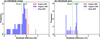 |
Fig. D.1 (a) Histograms of the difference between the residuals from wave-1 to wave-4 fits and those from wave-1 to wave-3 fits for the temperature field. (b) Same as (a), but for the pressure field. Residual differences in the pressure field are normalized by the maximum difference. |
Coverage-weighted agreement statistics for longitudinal wave components in temperature (T).
Coverage-weighted agreement statistics for longitudinal wave components in pressure (P).
All Tables
Coverage-weighted agreement statistics for longitudinal wave components in temperature (T).
Coverage-weighted agreement statistics for longitudinal wave components in pressure (P).
All Figures
|
Fig. 1 SPICAM data coverage used in this study. (a) Coverage in MYs for all available profiles. (b–f) Data coverage in local time, latitude, and solar longitude for (b) all profiles, (c) South-Low-Clear, (d) South-Mid-Clear, (e) South-Low-Dusty, and (f) North-Low-Dusty cases. The number of profiles is indicated by N. |
| In the text | |
|
Fig. 2 Longitudinal structures of SPICAM temperature observations for (a) South-Low-Clear, (b) South-Mid-Clear, (c) South-Low-Dusty, and (d) North-Low-Dusty. Panels (e)–(h) show the corresponding structures from sampled PCM data. Dots indicate data points and shaded regions represent ±1σ uncertainties of the composite fits. Panels (i) to (l) show the amplitudes and ±1σ uncertainties of waves 1–4, normalized by the zonal mean for the four cases in (a)–(d). For clarity, the SPICAM and sampled PCM profiles are vertically offset by +1 km and −1 km, respectively. The SPICAM amplitudes use dashed semi-transparent lines; PCM amplitudes use solid, opaque lines. Panels (m)–(p) show the corresponding phases and ±1σ uncertainties, defined as the longitude of the first eastward peak from 0◦ for each harmonic component. The temperature structures in the first two rows are vertically offset by [−100, −30, 30, 120, 200, 290] K for 80–130 km altitudes, except for the North-Low-Dusty case, which uses [−100, −30, 70, 210, 320, 450] K. |
| In the text | |
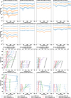 |
Fig. 3 Same as Figure 2, but for pressure. |
| In the text | |
|
Fig. 4 Amplitudes of temperature for different fit tidal modes and the zonal mean derived from the full PCM data for four cases: (a) South-Low-Clear, (b) South-Mid-Clear, (c) South-Low-Dusty, and (d) North-Low-Dusty. Panels (e)–(h) are similar to (a)–(d), but for the pressure field. The mode decomposition includes both tidal components and SPW contributions with the same zonal wavenumber. |
| In the text | |
|
Fig. 5 Wave-4 fit based on residuals obtained after subtracting the fit wave-1 to wave-3 components from SPICAM temperature and pressure observations for four cases: (a) South-Low-Clear, (b) South-Mid-Clear, (c) South-Low-Dusty, and (d) North-Low-Dusty. Dots and shaded regions represent the data points and ±1σ uncertainties, respectively. This residual-based analysis verifies that the wave-4 signal identified in the full harmonic fit is not an artifact of noise. |
| In the text | |
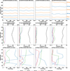 |
Fig. B.1 Same as Figure 2, but for the full PCM data set. |
| In the text | |
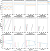 |
Fig. B.2 Same as Figure 3, but for the full PCM data set. |
| In the text | |
|
Fig. D.1 (a) Histograms of the difference between the residuals from wave-1 to wave-4 fits and those from wave-1 to wave-3 fits for the temperature field. (b) Same as (a), but for the pressure field. Residual differences in the pressure field are normalized by the maximum difference. |
| In the text | |
Current usage metrics show cumulative count of Article Views (full-text article views including HTML views, PDF and ePub downloads, according to the available data) and Abstracts Views on Vision4Press platform.
Data correspond to usage on the plateform after 2015. The current usage metrics is available 48-96 hours after online publication and is updated daily on week days.
Initial download of the metrics may take a while.