| Issue |
A&A
Volume 707, March 2026
|
|
|---|---|---|
| Article Number | A73 | |
| Number of page(s) | 22 | |
| Section | Planets, planetary systems, and small bodies | |
| DOI | https://doi.org/10.1051/0004-6361/202557656 | |
| Published online | 09 March 2026 | |
TOI-3288 b and TOI-4666 b: Two gas giants transiting low-mass stars characterised by NIRPS
1
Observatoire de Genève, Département d’Astronomie, Université de Genève,
Chemin Pegasi 51,
1290
Versoix,
Switzerland
2
European Southern Observatory (ESO),
Av. Alonso de Cordova 3107, Casilla
19001,
Santiago de Chile,
Chile
3
Institut Trottier de recherche sur les exoplanètes, Département de Physique, Université de Montréal, Montréal,
Québec,
Canada
4
Departamento de Física Teórica e Experimental, Universidade Federal do Rio Grande do Norte, Campus Universitário,
Natal,
RN
59072-970,
Brazil
5
Instituto de Astrofísica e Ciências do Espaço, Universidade do Porto, CAUP, Rua das Estrelas,
4150-762
Porto,
Portugal
6
Observatoire du Mont-Mégantic,
Québec,
Canada
7
Univ. Grenoble Alpes, CNRS, IPAG,
38000
Grenoble,
France
8
Centro de Astrobiología (CAB), CSIC-INTA, Camino Bajo del Castillo s/n,
28692
Villanueva de la Cañada (Madrid),
Spain
9
Light Bridges S.L., Observatorio del Teide, Carretera del Observatorio, s/n Guimar,
38500
Tenerife, Canarias,
Spain
10
Instituto de Astrofísica de Canarias (IAC), Calle Vía Láctea s/n,
38205
La Laguna, Tenerife,
Spain
11
Departamento de Astrofísica, Universidad de La Laguna (ULL),
38206
La Laguna, Tenerife,
Spain
12
Departamento de Física e Astronomia, Faculdade de Ciências, Universidade do Porto, Rua do Campo Alegre,
4169-007
Porto,
Portugal
13
Department of Earth, Planetary, and Space Sciences, University of California,
Los Angeles,
CA
90095,
USA
14
Department of Physics, University of Toronto,
Toronto,
ON
M5S 3H4,
Canada
15
Department of Physics & Astronomy, McMaster University,
1280 Main St W,
Hamilton,
ON
L8S 4L8,
Canada
16
Department of Physics, McGill University,
3600 rue University,
Montréal,
QC
H3A 2T8,
Canada
17
Department of Earth & Planetary Sciences, McGill University,
3450 rue University,
Montréal,
QC
H3A 0E8,
Canada
18
Centre Vie dans 1’Univers, Faculté des sciences de l’Université de Genève,
Quai Ernest-Ansermet 30,
1205
Geneva,
Switzerland
19
European Southern Observatory (ESO),
Karl-Schwarzschild-Str. 2,
85748
Garching bei München,
Germany
20
Space Research and Planetary Sciences, Physics Institute, University of Bern,
Gesellschaftsstrasse 6,
3012
Bern,
Switzerland
21
Consejo Superior de Investigaciones Científicas (CSIC),
28006
Madrid,
Spain
22
Bishop’s University, Dept of Physics and Astronomy,
Johnson-104E, 2600 College Street,
Sherbrooke,
QC
J1M 1Z7,
Canada
23
Department of Physics, Engineering Physics, and Astronomy, Queen’s University,
99 University Avenue,
Kingston,
ON
K7L 3N6,
Canada
24
Department of Physics and Space Science, Royal Military College of Canada,
13 General Crerar Cres.,
Kingston,
ON
K7P 2M3,
Canada
25
Astrobiology Research Unit, Université de Liège,
19C Allée du 6 Août,
4000
Liège,
Belgium
26
Department of Earth, Atmospheric and Planetary Sciences, Massachusetts Institute of Technology,
Cambridge,
MA
02139,
USA
27
Center for astrophysics | Harvard & Smithsonian,
60 Garden Street,
Cambridge,
MA
02138,
USA
28
Caltech/IPAC,
Mail Code 100-22,
Pasadena,
CA
91125,
USA
29
Department of Astronomy, Westlake University,
Hangzhou
310030, Zhejiang Province,
PR
China
30
NASA Ames Research Center,
Moffett Field,
CA
94035,
USA
31
University Observatory, Faculty of Physics, Ludwig-Maximilians-Universität München,
Scheinerstr. 1,
81679
Munich,
Germany
32
Department of Astronomy & Astrophysics, University of Chicago,
5640 South Ellis Avenue,
Chicago,
IL
60637,
USA
33
Department of Physics and Astronomy, Vanderbilt University,
VU Station 1807,
Nashville,
TN
37235,
USA
34
SETI Institute,
Mountain View, CA 94043, USA NASA Ames Research Center,
Moffett Field,
CA
94035,
USA
★ Corresponding author: This email address is being protected from spambots. You need JavaScript enabled to view it.
Received:
10
October
2025
Accepted:
20
December
2025
Abstract
Context. Gas giant planets orbiting low-mass stars (Teff ≲ 4600 K) are uncommon outcomes of planet formation. Increasing the sample of well-characterised giants around early M dwarfs will enable population-level studies of their properties, offering valuable insights into their formation and evolutionary histories.
Aims. We aim to confirm and characterise giant exoplanets transiting M dwarfs identified by the TESS mission. To this end, we have started the Gas giAnts Transiting 1Ow-mass Stars (GATOS) programme within the NIRPS guaranteed time observations (GTO).
Methods. High-resolution spectroscopic data were obtained in the optical and near-infrared (nIR), combining HARPS and NIRPS. We derived radial velocities (RVs) via the cross-correlation function and implemented a novel post-processing procedure to further mitigate telluric contamination in the nIR. The resulting RVs were jointly fit with TESS and ground-based photometry to derive the orbital and physical parameters of the systems.
Results. We present the GATOS programme and its first results. We confirm two gas giants transiting the low-mass stars TOI-3288 A (K9V, Teff = 3933 ± 48 K) and TOI-4666 (M2.5V, Teff = 3512 ± 36 K). TOI-3288 A hosts a hot Jupiter with a mass of 2.11 ± 0.08 MJup and a radius of 1.00 ± 0.03 RJup, with an orbital period of 1.43 days (Teq = 1059 ± 20 K). TOI-4666 hosts a 0.70 ± 0.06 MJup warm Jupiter (Teq = 713 ± 14 K) with a radius of 1.11 ± 0.04 RJup, with an orbital period of 2.91 days. At a population level, we identify a decrease in planetary mass with spectral type, whereby late M dwarfs host less massive giant planets than early M dwarfs. More massive gas giants that deviate from this trend are preferentially hosted by more metal-rich stars. Furthermore, we find an increased binarity fraction among low-mass stars hosting gas giants, which may play a role in enhancing giant planet formation around low-mass stars.
Conclusions. These mass characterisations contribute to the growing catalogue of well-defined giant exoplanets around low-mass stars. The observed population trends agree with theoretical predictions, whereby higher metallicity can compensate for lower disc masses, and wide binary systems may influence planet formation and migration through Kozai–Lidov cycles or disc instabilities.
Key words: techniques: photometric / techniques: radial velocities / planets and satellites: gaseous planets / stars: individual: TOI-3288 / stars: individual: TOI-4666
© The Authors 2026
 Open Access article, published by EDP Sciences, under the terms of the Creative Commons Attribution License (https://creativecommons.org/licenses/by/4.0), which permits unrestricted use, distribution, and reproduction in any medium, provided the original work is properly cited.
This article is published in open access under the Subscribe to Open model. This email address is being protected from spambots. You need JavaScript enabled to view it. to support open access publication.
1 Introduction
Jupiter-mass planets are scarce around M dwarfs, and theoretical models for a time predicted that stars with masses below 0.5 M⊙ would have none (Burn et al. 2021). Both core accretion and gravitational instability – the leading mechanisms of giant planet formation – are hindered by the low disc surface densities, extended disc orbital timescales, and generally low disc masses around M dwarfs (Laughlin et al. 2004; Ida & Lin 2005). The combination of limited material and slow disc orbital motion hinders the accumulation of solids and gas, preventing cores from reaching the critical mass needed for rapid gas accretion (core accretion) or for the disc to fragment (gravitational instability), and thus limiting giant planet formation before the disc disperses.
However, an increasing number of giant planets are being detected around low-mass stars (e.g. Marcy et al. 1998; Morales et al. 2019; Parviainen et al. 2021; Bryant et al. 2025). Recent studies based on photometric data from the Transiting Exoplanet Survey Satellite (TESS; Ricker et al. 2014) show an occurrence rate of 0.27 ± 0.09% for the stellar mass range 0.45–0.65 M⊙ (Gan et al. 2023), and demonstrate that giant planets exist around stars with M⋆ ≤ 0.4 M⊙ (Bryant et al. 2023). Radial-velocity surveys consistently show that short-period (1–10 d), Jupiter-mass planets are uncommon but exist around M dwarfs, with recent studies placing their occurrence rate below about 2% (e.g. Ribas et al. 2023; Bonfils et al. 2013; Pinamonti et al. 2022; Pass et al. 2023; Mignon et al. 2025). These findings raise the question of whether a stellar mass threshold exists below which giant planet formation becomes impossible. Observational biases have prevented us from clearly identifying the point at which giant planet formation starts to decline, as faint M dwarfs (V ≥ 14 mag) are generally not observable with optical ground-based spectrographs. With the advent of near-infrared (nIR) spectrographs such as the Near-InfraRed Planet Searcher (NIRPS; Bouchy et al. 2025), radial velocity (RV) surveys can now be extended to fainter M dwarfs that were previously less accessible.
However, the nIR introduces challenges not as strongly encountered in the visible. At the faint end, limitations from telluric absorption and emission lines arise, especially when the Barycentric Earth Radial Velocity (BERV) is similar to the star’s systemic velocity, causing the telluric and stellar lines to overlap. Giant planets around low-mass stars induce significant RV variations due to their stronger gravitational pull, allowing observations of fainter stars than those targeted in searches for less massive planets. As a by-product, this makes them ideal targets for assessing the performance of NIRPS on faint M dwarfs and for better understanding its faint-end limits.
To determine the stellar mass threshold at which giant planet formation declines, an ongoing NIRPS guaranteed time observations (GTO) sub-programme is characterising gas giants and brown dwarfs transiting low-mass stars to expand the known sample. In this paper, we confirm and characterise two gas giants, contributing new mass measurements to this still relatively unexplored population. We present the ongoing sub-programme (Sect. 2), and propose a new method of improving the precision of faint nIR observations affected by telluric contamination (Sect. 5). The first two gas giant confirmations of the programme are detailed in Sects. 3, 4, and 6, covering the observations, stellar characterisation, and orbital solutions, respectively.
2 NIRPS GTO TESS Follow-Up: Gas giAnts Transiting IOw-mass Stars (GATOS)
As part of the ongoing NIRPS GTO, this programme aims to characterise giant planets identified by the Transiting Exoplanet Survey Satellite (TESS; Ricker et al. 2014) orbiting M dwarfs. Observations began with the start of NIRPS operations in April 2023, with some targets having been observed during the commissioning phase to test the instrumental magnitude limits. The target selection is summarised as follows:
We searched for all TESS objects of interest (TOIs) with a planetary radius of 7.5 R⊕ < Rpl < 16 R⊕ that orbit M dwarfs, defined as stars with effective temperatures of 2310 K < Teff < 3930 K1, resulting in 193 TOIs. The lower radius limit excludes strongly inflated Neptunes that produce small RV signals and are hard to characterise around faint stars. As the stars are cool, strongly inflated gas giants are not expected; the upper limit therefore excludes eclipsing binaries (EBs) around low-mass stars.
We excluded 33 targets that were previously characterised planets or brown dwarfs, as well as 49 false positive (FP) signals, and 2 false alarms. The FPs were identified by having a TESS Follow-up Observing Program (TFOP) working group (WG) disposition of ambiguous planet candidates, EBs, or nearby planet candidates (i.e. transits associated with the ‘wrong’ star). We only excluded cases in which a binary causes the transit; binary star systems hosting a transiting planet were included.
Of the remaining 109 stars, 54 are observable from La Silla Observatory (δ ≤ + 20°), of which just 14 meet the magnitude constraints we imposed for NIRPS follow-up (J ≤ 12.5 and H ≤ 12.5). These magnitudes roughly correspond to the limits at which ~10–20 40-minutes NIRPS exposures can yield a 5σ mass characterisation of short-period gas giants.
These 14 were then individually vetted through inspections of their light curves and the notes from the TESS Spectroscopic Follow-Up WG. We excluded potential EBs, indicated by odd-even transit depth differences, secondary eclipses, or wavelength-dependent transit depth variations. V-shaped transits were kept, as they might reflect a grazing planetary transit. Such transits are more likely when larger companions transit small-sized stars. In addition to the vetting performed by TESS, we visually vetted the light curves before including targets in our programme. Additionally, if another facility or team was planning high-precision spectroscopic follow-up observations, we did not initiate our own. In total 3 of the 14 were rejected, and 2 studied by other teams.
The number of stars reported above reflects the coordinated observations table of the TESS Spectroscopic Follow-up WG downloaded on 12 August 2025. These values have evolved since the 2023 start of our programme: in January 2023, 77 TOIs matched our planetary radius and effective temperature criteria, which has since increased by 116 thanks to the continuous effort of the Quick Look Pipeline (QLP) Faint search team (Kunimoto et al. 2022). Some of the targets now listed as FPs were identified by our programme, such as the spectroscopic binaries TOI-2341 and TOI-5295 (see Appendix A). The programme observed some fast-rotating stars that may still host planets, but their broadened cross-correlation functions (CCFs) prevent precise RV determination (see Appendix B).
To vet against stars that have evolved away from the main sequence, we plot the targets of this sub-programme on the Gaia DR3 (Gaia Collaboration 2023) HR diagram for nearby stars (d ≤ 200 pc; Fig. 1). The two stars discussed in this paper are on the main sequence, while some now discarded targets turned out to be evolved giant stars (see Appendix C for more details on why these were excluded from the sample).
We first obtained two spectroscopic observations for all of our targets, to promptly reject EBs identifiable by large RV variations and/or multiple components in their CCF. We increased the observation frequency if no binarity was observed.
The NIRPS Exposure Time Calculator (ETC)2 was used to estimate the precision achievable under optimal conditions, helping to approximate the number of observations required to achieve a ~5σ mass characterisation for planets of ≳0.5 MJup. The ETC is based on commissioning data taken during nominal weather conditions; therefore, it provides optimistic predictions.
This work reports on the first two targets (TOI-3288 and TOI-4666) for which the RVs confirm the presence of gas giants. We present their observations and analysis in the following sections.
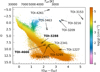 |
Fig. 1 HR diagram of all Gaia DR3 nearby stars with a parallax of π ≥ 5 mas, using the broad-band G magnitude versus the colour GBP (blue) minus GRP (red). The colours indicate log(g). Stars without a log(g) measurement are shown in grey. The six targets presented in this paper as part of the NIRPS-GTO giants sub-programme are overplotted (outlined black circles), along with five stars identified as giant stars using this method. TOI-3288 and TOI-4666 (outlined black squares), hosting gas giants, are visible on the main sequence. This figure can be generated using Gaia-HR, available at https://github.com/ygcfrensch/Gaia-HR. |
Properties of the TESS extracted light curves.
3 Observations
3.1 TESS photometry
TOI-3288.01 was alerted on 4 June 2021 (Guerrero et al. 2021) by the TESS Science Office (TSO) after the FAINT transit search pipeline (Kunimoto & Daylan 2021) detected the planet candidate, using the Quick Look Pipeline (QLP; Huang et al. 2020b,a) on the full frame image (FFI) data from sectors 13 and 27. The SPOC transit search pipeline (Jenkins 2002; Jenkins et al. 2010, 2020) later measured the transit signature in higher-cadence data from sector 67. Similarly, the FAINT pipeline detected the candidate TOI-4666.01 using the QLP FFI light curve from sector 31. After its standard series of automated and manual vetting steps (e.g. Twicken et al. 2018; Li et al. 2019), the TSO issued a TOI alert on 21 December 2021. Table 1 presents the sectors in which TESS observed TOI-3288 and TOI-4666 together with the photometric cadences and out-of-transit scatters. TESS’s simple aperture photometry (SAP) is affected by instrumental systematic effects mostly originating from the spacecraft pointing, which have been shown to be effectively corrected through the PDC algorithm originally developed for the Kepler mission (see Stumpe et al. 2012, 2014; Smith et al. 2012; Kinemuchi et al. 2012). The PDC-corrected SAP (i.e. PDCSAP) is delivered by the SPOC and TESS-SPOC pipelines for a series of TESS sectors. Unfortunately, for our targets, only sector 67 for TOI-3288 has available PDCSAP data. Therefore, we consistently extracted our own PDCSAP photometry from the FFIs (which we accessed through the lightkurve Python package; Lightkurve Collaboration 2018) in a similar manner to the TESS-SPOC pipeline. First, we excluded any FFI flagged for quality issues, recognisable by a non-zero quality parameter. Then, we built the photometric apertures. As both stars are in crowded fields, we used the TESS-cont algorithm3 (Castro-González et al. 2024) to create apertures that minimise the flux from nearby contaminant stars, restricting them to those pixels where at least 60% of the flux originates from the target star (see Appendix K for the selected apertures). We subsequently obtained the SAP photometry by subtracting the background flux, which we obtained by defining a background aperture as the nearby pixels with median flux lower than the minimum flux plus 2.5% of the standard deviation, excluding all pixels which belong to the aperture mask. Finally, we applied the cotrending basis vectors (CBV) corrector implemented in lightkurve and corrected from crowding through the CROWDSAP and FLFRCSAP metrics computed by TESS-cont for the selected apertures. (the photometric data are presented in Appendix I).
3.2 Zorro speckle interferometry
If a star hosting a planet candidate has a close bound binary companion or a background star that is angularly close in the line of sight, the additional light falling within the photometric aperture can create a FP exoplanet detection due to the effect on the transit depth (e.g. Ciardi et al. 2015; Cabrera et al. 2017) or corrupt the determined parameters for both the planet and host star (e.g. Furlan & Howell 2017, 2020; Castro-González et al. 2022). We could obtain high-resolution optical speckle imaging observations to search for close-in companions unresolved in TESS or other follow-up observations for TOI-3288, but not for TOI-4666.
TOI-3288 was observed on 17 May 2022 UT using the speckle instrument Zorro on the Gemini South 8-m telescope (Scott et al. 2021). Zorro provides simultaneous speckle imaging in two bands (562 nm and 832 nm) with output data products including a reconstructed image with robust contrast limits on companion detections. Thirteen sets of 1000 × 0.06 sec exposures were collected and subjected to Fourier analysis in our standard reduction pipeline (Howell et al. 2011). Figure 2 shows our final 5 σ magnitude contrast curves and the reconstructed speckle images. We find that TOI-3288 does not have a stellar companion brighter than 4.5 to 6.4 magnitudes below that of the target star from the diffraction limit (20 mas) out to 1.2″. At the distance of TOI-3288 (d = 200 pc), these angular limits correspond to spatial limits of 4–240 AU. Beyond the 1.2" field probed by Zorro, Gaia reveals a stellar companion at ~2.3″ (Gaia DR3 6685431748040148992) with G = 17.2 mag, which is discussed in more detail in Sect. 7.3.
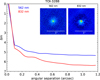 |
Fig. 2 5 σ magnitude contrast curves as observed by Zorro in both filters as a function of the angular separation out to 1.2″. The insets show the reconstructed speckle images of TOI-3288 with a 1″ scale bar. TOI-3288 was found to have no close companions from the diffraction limit (0.02″) out to 1.2″ to within the magnitude contrast levels achieved. |
3.3 Ground-based photometry
To determine the true source of the TESS detection, we acquired ground-based time-series follow-up photometry of the fields around TOI-3288 and TOI-4666 as part of the TESS Follow-up Observing Program (TFOP; Collins 2019)4. We used the TESS Transit Finder, which is a customised version of the Tapir software package (Jensen 2013), to schedule our transit observations. The light curve data are available on the EXOFOP-TESS website5 and are included in the global modelling described in Sect. 6. TOI-3288 was observed with LCOGT and TOI-4666 with ExTrA, as part of the coordinated photometric follow-up to validate the transit, depending on the availability of the facilities.
3.3.1 LCOGT – TOI-3288
The Las Cumbres Observatory Global Telescope (LCOGT; Brown et al. 2013) 1.0 m and 0.4 m network nodes used in the TOI-3288 observations are located at Cerro Tololo Inter-American Observatory in Chile (CTIO), Siding Spring Observatory near Coonabarabran, Australia (SSO), and South African Astronomical Observatory near Cape Town South Africa (SAAO). The 1 m telescopes are equipped with 4096 × 4096 SINISTRO cameras that have an image scale of 0.389″ per pixel, resulting in a 26′ × 26′ field of view. The 0.4 m telescopes are equipped with a 2048 × 3072 pixel SBIG STX6303 camera that has an image scale of 0.57″ pixel−1, resulting in a 19′ × 29′ field of view. The standard LCOGT BANZAI pipeline (McCully et al. 2018) calibrated all LCOGT images, and differential photometric data were extracted using AstroImageJ (AIJ; Collins et al. 2017). All observations of TOI-3288 are affected by contamination from the stellar companion Gaia DR3 6685431748040148992.
3.3.2 ExTrA – TOI-4666
ExTrA (Exoplanets in Transits and their Atmospheres, Bonfils et al. 2015) is a low-resolution nIR (0.85 to 1.55 μm) multi-object spectrograph fed by three 60-cm telescopes located at La Silla Observatory in Chile. A total of ten transits of TOI-4666 b were observed using two (two transits) or three (eight transits) of the ExTrA telescopes. We used 8″ diameter aperture fibres and the low-resolution mode (R ~ 20) of the spectrograph, with an exposure time of 60 seconds. Five fibres are positioned in the focal plane of each telescope to select light from the target and four comparison stars. The resulting ExTrA data were analysed using custom data reduction software (Cointepas et al. 2021).
3.3.3 ASAS-SN
We complemented the dataset using observations from the All Sky Automated Survey for SuperNovae (ASAS-SN; Kochanek et al. 2017), an automated photometric programme that looks out for supernovae and other transient events. ASAS-SN is a network of 24 ground-based 14-centimetre telescopes distributed over six sites. Due to their cadence, these data are not used to detect transit events but instead to follow the stars’ behaviour. We obtained ~8 years of g-band photometry and ~ 4.5 years of V-band photometry of both targets. Before analysing it, the data were nightly binned and linearly detrended from long-term variations.
3.4 HARPS and NIRPS spectroscopy
NIRPS is an adaptive optics (AO)-assisted and fibre-fed high-resolution spectrograph operating at the ESO 3.6-meter telescope in La Silla Observatory. It had its first light in May 2022 (Wildi et al. 2022; Artigau et al. 2024; Bouchy et al. 2025). NIRPS observes the nIR (λ = 0.98–1.8 μm). Fibre modal noise is more dominant and can severely limit the highest signal-to-noise ratio (S/N) achievable on bright stars (S/N; Iuzzolino et al. 2014). NIRPS combines fibre stretchers, octagonal fibres, double scramblers, and AO tip-tilt scrambling (Blind 2022; Frensch et al. 2022) to significantly reduce modal noise. Simultaneous observations are possible with HARPS (High-Accuracy Radial Velocity Planetary Searcher; Mayor et al. 2003), which covers the optical range (λ = 0.38–0.69 μm).
NIRPS uses a high-order AO system to couple starlight into four relatively small multi-mode fibres (29-μm and 66-μm). There are two observing modes: high accuracy (HA) and high efficiency (HE), both of which include one science fibre and one reference fibre. For the faint targets in the giants programme, we used the HARPS-EGGS (HE) and NIRPS-HE modes to maximise throughput and minimise modal noise. During the period that the EGGS shutter was malfunctioning (~June to late September 2024), we performed observations in the HARPS-HAM (HA) mode instead. The reference fibre for NIRPS is pointed at the sky; these simultaneous sky observations are used to correct for telluric lines. As both instruments are ultra-stable, continuous drift monitoring is not required.
The stellar spectra for HARPS and NIRPS were extracted using version 3.2.0 of the NIRPS Data Reduction Software (DRS) adapted from the ESPRESSO DRS (Pepe et al. 2021). For NIRPS, the DRS includes corrections for telluric absorption and emission (Allart et al. 2022, Srivastava et al., A&A, in review). To correct telluric absorption, a synthetic spectrum was created. First, the CCF was computed to obtain an average telluric line per molecule. Using physical parameters from the HITRAN database (Gordon et al. 2022), a model was fitted to each average line. The fitted parameters were then used to generate the synthetic telluric spectrum, which was subtracted from the observations. Telluric emission was corrected by scaling lines from the reference fibre to the science fibre using ratios determined from previous sky–sky observations. For HARPS, the DRS does not correct for telluric contamination as the optical domain is less affected. These corrections are sufficient to enable sub-metre-per-second precision for bright targets, such as Proxima (Suárez Mascareño et al. 2025); however, fainter targets require some additional cleaning to improve precision and accuracy. In Sect. 5, we discuss the technique used to further reduce telluric contamination.
The line-by-line (LBL; Dumusque 2018; Artigau et al. 2022) method of determining RV measurements has been optimised to handle spectral outliers and to minimise their impact. Radial velocities are measured independently in all valid lines (typically ~16 000 in NIRPS), and an error-weighted average is computed that accounts for outliers through a finite-mixture model. This produces a soft clipping (a gradually decreasing weight) at the 4–5 σ level. In the presence of uncorrelated outliers, this method significantly outperforms CCF measurements (see Figures 5 and 6 in Artigau et al. 2022).
A key limiting case arises when numerous lines are distorted in a correlated manner, at low-enough significance to avoid rejection by the finite-mixture model, yet in sufficient numbers to significantly bias the combined RV. This is particularly the case in low-S/N observations of targets that have a low systemic velocity, which is the case here. Since all water lines are affected in a correlated way by finite-resolution effects (see Figures 4 and 5 in Wang et al. 2022), there is a bulk effect that cannot be mitigated by rejecting individual outliers. This occurs when water absorption lines overlap within a few kilometres per second with water lines in cool dwarfs, i.e. when the sum of the barycentric correction and the systemic velocity of the star is within about one resolution elements of zero (i.e. <5 km/s). Not all observed stars are affected, as this depends on their systemic velocity and ecliptic latitude.
This correlated effect must be addressed either through improved telluric correction (i.e. better accounting of finite-resolution effects and refined telluric line profiles) or through parametrisation of its impact on the mean line profile (see Parc et al. 2025, for a strategy where OH lines are removed). While the former approach is the focus of ongoing work, in the present analysis we opted for the latter.
We concentrated on post-processing the CCF RVs to develop CCF-specific mitigation techniques, complementing the available LBL strategies. Table 2 summarises the characteristics of the post-processed observations, and the individual RVs are presented in Appendix H. The NIRPS RVs were obtained in three consecutive 800 s sub-exposures to reduce instrumental systematics. Since the individual sub-exposures do not reach the required precision, they were combined into a single RV measurement, which we refer to as ‘night-binning’ throughout the paper.
4 Stellar properties
Table 3 summarises the stellar parameters of TOI-3288 and TOI-4666. The TIC working group (Paegert et al. 2021; Stassun et al. 2019) magnitudes are reported. The J, H, and K magnitudes follow from 2MASS (Cutri et al. 2003). The V magnitudes were calculated from the Gaia colours (G, B′, R′) and the B magnitudes were calculated following Stassun et al. (2018), as the stars are too faint to be included in the Tycho catalogue (ESA 1997). Surface gravities, log g, parallaxes, π, and corresponding distances, d, originate from Gaia DR3 (Gaia Collaboration 2023). Effective temperatures, Teff, and abundances, [X/H], were determined through a spectral analysis of NIRPS and HARPS data to ensure consistency between the independently obtained values; see Sect. 4.1 for details. Spectral types were inferred from the NIRPS Teff using Table 5 of Pecaut & Mamajek (2013). The extinction, AV, and bolometric luminosity, Lbol, were derived from an SED fit (Sect. 4.2). From empirically appropriate relations, the stellar radius and mass were estimated in the manner described by Mann et al. (2015, 2019) for Teff < 4000 K. For TOI-3288 the K band is contaminated by the nearby stellar companion, which is 16 times fainter than the primary. The contamination is low, but impacts the inferred R⋆ and M⋆. The TESS light curves show possible rotational modulations, which allow us to estimate rotation period, Prot (Sect. 4.3).
Properties of the TESS extracted light curves.
4.1 Spectral analysis
4.1.1 NIRPS
For each star, the spectroscopic stellar parameters were derived from a single high-resolution template spectrum, obtained by combining the individual telluric-corrected spectra from the APERO DRS (Cook et al. 2022). We note that the resulting templates have low S/N (54 and 67 for TOI-3288 and TOI-4666, respectively). Following the methodology of Jahandar et al. (2024, 2025), we first determined the effective temperature, Teff, and overall metallicity, [M/H], by fitting groups of spectral features to a pre-generated grid of PHOENIX ACES stellar models (Husser et al. 2013). The models were convolved to the resolution of NIRPS and have log g = 4.50, as both stars have surface gravities within 0.2 dex of this value (see Table 3), where variations in log g do not affect the spectral analysis. We find Teff = 3933 ± 48 K and [M/H] = −0.1 ± 0.1 dex for TOI-3288, while the TOI-4666 spectrum yields Teff = 3512 ± 36 K and [M/H] = −0.1 ± 0.1 dex. We note that the effective temperature of TOI-3288 classifies it as a K9. This discrepancy arises because the TESS Input Catalog (TICv8; Stassun et al. 2019) often relies on empirical color-based relations, whereas the spectral analysis presented here is based on direct observations.
To measure the abundances of individual chemical species, we then performed fits on individual spectral lines, using a PHOENIX grid with fixed Teff of 3940 K and 3520 K for TOI-3288 and TOI-4666, respectively (Jahandar et al. 2024, 2025). Due to the low S/N of the templates, we were only able to fit very few lines per element; all reported abundances are based on at least three lines (see Table 3). To determine the uncertainty on the abundance measurements, we took the dispersion of the individual measurements. We note that the overall metallicities reported for both stars ([M/H] = −0.1 ± 0.1 dex; see Table 3) are values typically considered as a first approximation of [M/H]. Being measured directly from the spectrum, this [M/H] is affected by the relative number of lines of the different chemical species. For M dwarfs in the nIR, the spectrum is often dominated by OH lines, resulting in a spectral [M/H] that can differ from one measured at optical wavelengths, where Fe lines are more prominent. To account for this difference, we typically would report an integrated [M/H], defined as an average of the abundance of each element (Jahandar et al. 2024). Because of the low S/N and small number of measured chemical species (three for TOI-3288 and only one for TOI-4666, see Table 3), we decided to instead report the [M/H] based on the overall stellar spectrum.
Stellar parameters of the stars presented in this paper.
4.1.2 HARPS
In addition, we derived Teff and metallicity [Fe/H] (i.e. iron abundance) from the HARPS spectrum using the machine learning tool ODUSSEAS6 (Antoniadis-Karnavas et al. 2020, 2024). We first combined all the individual HARPS spectra with the task scombine within IRAF7 to obtain a higher-S/N spectrum. This spectrum is used by ODUSSEAS to measure the pseudo-EWs of more than 4000 lines to apply a machine learning model trained with the same lines, measured and calibrated on a reference sample of 47 M dwarfs observed with HARPS for which their [Fe/H] were obtained from photometric calibrations (Neves et al. 2012) and their Teff from interferometric calibrations (Khata et al. 2021). We note that given the low S/N of the individual spectra for TOI-4666 we only used the cleaned spectra missing the bluest and reddest orders, which causes a reduction of 13% of the number of lines measured. With this method, we derived Teff = 3881 ± 111 K and [Fe/H] = 0.27 ± 0.13 dex for TOI-3288 and Teff = 3720 ± 103 K and [Fe/H] = 0.19 ± 0.12 dex for TOI-4666. The combined measurements from HARPS and NIRPS suggest that both stars are metal-rich but it is hard to have a good constraint on the real metallicity given the low S/N of the spectra. This prevents the derivation of an accurate temperature for TOI-4666, as is shown by the ~2 σ discrepancy between the value found with respect to the one obtained from the NIRPS spectrum. Therefore, these parameter values have to be taken with care.
4.2 SED analysis
The bolometric flux, Fbol, and extinction, AV, reported in Table 3 were obtained from an independent broadband spectral energy distribution (SED) analysis with the Gaia DR3 parallaxes (no systematic offset is applied; see, e.g. Stassun & Torres 2021). The JHKS magnitudes follow from 2MASS, the W1–W3 magnitudes from WISE, the GBP, GRP magnitudes from Gaia, and the absolute flux-calibrated Gaia spectrophotometry. The available photometry spans the full stellar SED over the wavelength range of 0.4–10 μm (see Figure D.1).
We fitted PHOENIX stellar atmosphere models (Husser et al. 2013) with the effective temperature, Teff, from NIRPS, and the surface gravity, log g, and metallicity, [Fe/H], set to the spectroscopically determined values from Sect. 4.1. The fit’s AV is limited by the maximum line-of-sight value from the Galactic dust maps of Schlegel et al. (1998). The Fbol at Earth was determined by integrating the unreddened model SED. Combining the Fbol and the parallax provides the bolometric luminosity, Lbol.
4.3 Rotational period
The raw TESS light curves (SAP flux) and detrended flux from the QLP light curves were analysed using three different periodicity analysis techniques: (i) Lomb–Scargle periodograms (e.g. Scargle 1982; Horne & Baliunas 1986; Press & Rybicki 1989), (ii) fast Fourier transform (FFT; see Zhan et al. 2019, for details), and (iii) wavelet analysis (Grossmann & Morlet 1984). We searched for variability signatures by considering periods from the Nyquist frequency (minimum period) up to 30 days, given that each TESS sector observes the sky for ~27 days. Diagnostic plots were constructed for each star, combining the light curves and results from all three methods to provide a more robust visual analysis. This enables the more accurate identification of consistent periodicities and facilitates the classification of stellar variability types. Our approach follows the same procedure described in Canto Martins et al. (2020).
As the rotation periods are similar across the various sectors and three techniques, we report weighted mean values of ~13.7 days for TOI-3288 and ~15.3 days for TOI-4666 (see Table 3). The value for TOI-3288 requires caution. Its three sectors exhibit complex patterns, which makes it difficult to attribute the variability to a consistent astrophysical origin. Since the behaviour of the light curves is not consistent with any known modulation reported in the literature, we cannot confidently conclude that the observed variability is astrophysical. In such cases, we follow the classification scheme from Canto Martins et al. (2020), where the variability is labelled as ‘ambiguous variation’.
To confirm the rotation measurements obtained from the TESS observations, we analysed the ASAS-SN data. We used a generalised Lomb-Scargle periodogram (Zechmeister & Kürster 2009) to evaluate the presence of periodic signals in the data. For TOI-3288 we detected a significant signal in the g-band data with a period of 16.3 days. The V-band data showed a signal at the same period, although not significant. The measurement differs from the TESS period. However, complexity of the sector-by-sector variation in the TESS data, combined with the fact that the sectors are spaced a year or more apart, might be obscuring the true astrophysical periodicity. For TOI-4666 we identified a non-significant signal in the g-band data with a period of 15.4 days, consistent with the period measured in the TESS light curve. Figures L.1 and L.2 shows the g-band data, and their respective periodograms, of TOI-3288 and TOI-4666.
5 Telluric mitigation and order selection
If the systemic velocity, vsys, and BERV overlap, Earth’s atmospheric lines blend with the stellar lines, which translates into a blended CCF containing contributions from both the RV signal and residual telluric features. The DRS telluric corrections already significantly reduce the contamination; however, fainter targets can still be heavily influenced. Allart et al. (2022) used the CCF method to compute average telluric lines, from which a reconstructed telluric spectrum was derived. At low S/N, the average telluric lines are poorly defined, which results in an inaccurate reconstructed spectrum, and thus in residuals or over-corrections in the final data. The S/N reaches only ~12 in the reddest orders for both TOI-3288 and TOI-4666.
To reduce the remnant effect, we introduced an additional post-processing step. First, the CCFs were computed similarly to the DRS using the iCCF Python package8 (Faria 2025). The spectra were cross-correlated with numerical stellar masks, closely matched to the spectral types of each TOI (M1 for NIRPS and M2 for HARPS) (Fellgett 1953; Baranne et al. 1996). From the full CCF, we estimated the FWHM. Then, for each NIRPS frame, we identified the BERV and removed all CCF values within the BERV ![Mathematical equation: $\[\left(\pm ~\frac{1}{2} \mathrm{FWHM}\right)\]$](/articles/aa/full_html/2026/03/aa57656-25/aa57656-25-eq4.png) window from the RV array. A Gaussian is fit to the remaining, BERV-excluded CCF, resulting in an uncontaminated RV value (see Fig. 3 for an illustration of the approach). This method works particularly well for very faint, heavily contaminated targets. However, it is not recommended for brighter stars, as significant information is lost in the process (e.g. flux from uncontaminated orders is also excluded). For the joint fit presented in Sect. 6, we use the RVs obtained from this technique.
window from the RV array. A Gaussian is fit to the remaining, BERV-excluded CCF, resulting in an uncontaminated RV value (see Fig. 3 for an illustration of the approach). This method works particularly well for very faint, heavily contaminated targets. However, it is not recommended for brighter stars, as significant information is lost in the process (e.g. flux from uncontaminated orders is also excluded). For the joint fit presented in Sect. 6, we use the RVs obtained from this technique.
For HARPS, another approach was used: orders 1 to 30 were excluded due to the critically low S/N in the blue, and the two reddest orders were removed to avoid potential telluric contamination. The remaining orders were summed to compute the final CCF, following the standard DRS procedure.
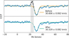 |
Fig. 3 Normalised CCF of TOI-3288. The upper panel shows the full CCF, while the lower panel shows the CCF with the BERV window |
![Mathematical equation: $\[\left(\pm \frac{1}{2} \mathrm{FWHM}\right)\]$](/articles/aa/full_html/2026/03/aa57656-25/aa57656-25-eq3.png)
6 Orbital solution
We combined the post-processed RVs with the photometric data using the Juliet Python package (Espinoza et al. 2019), applying dynesty (Speagle 2020) for dynamic nested sampling to estimate Bayesian posteriors and evidences. A joint fit was performed, combining the NIRPS and HARPS RVs with all available photometric data. The resulting orbital solution is presented in this section. We did not include a Gaussian process (GP) regression, as the stellar rotation period is poorly constrained. In addition, we fitted the HARPS and NIRPS data separately using photometric priors on the epoch and orbital period, and compared the derived semi-amplitudes to verify consistency between the optical and nIR. A mismatch could indicate a diluted EB.
The priors used for the joint fit are presented in Table G.1. The prior values for the orbital period, P, time of transit, T0, and stellar density, ρ⋆, were retrieved from the ExoFOP website5. We adopted priors with broad bounds to ensure that they are relatively uninformative. The eccentricity, e, and argument of periastron, ω, were either fixed (e = 0, ω = 90°), or e was modelled using a beta prior following Kipping (2013), while ω was assigned a uniform prior between 0° and 180°. The models were compared using the log-evidence to determine whether fixing e and ω or allowing them to vary provides a better fit to the data. A uniform prior between 0 and 1 was applied to the radius ratio (Rpl/R⋆) and impact parameter (b). Since the transits are not V-shaped, and thus not grazing, values of b greater than 1 are outside the considered range. All other priors follow the recommendations from the Juliet documentation. The resulting posterior distributions are presented as corner plots in Appendix J (Foreman-Mackey 2016).
The integrated AO guiding camera images are available with each observation. These can be inspected for contaminating sources in the RV observations (Appendix E). The TESS light curves were corrected for contamination. However, as TOI-3288 has a stellar companion, a dilution factor, D, is included as a uniform prior from 0.1 to 1 for the ground-based photometry. As the ExTrA light curves of TOI-4666 were extracted with an 8″ diameter aperture, and the closest star lies at 38″, contamination is negligible. Therefore, the dilution factor was fixed to 1. Each ExTrA transit and telescope was treated as a separate instrument, sharing only the limb darkening coefficients. The ground-based follow-up photometry of TOI-3288 was detrended for airmass using a linear regression model. For the ExTrA data, we instead used a GP with a Matérn kernel to model correlated noise.
The orbital solutions from the joint fit with Juliet are presented in Table 4. The fitted parameters were directly obtained from the model, with reported uncertainties corresponding to the 1σ errors. Instrument-specific parameters, also derived from the model, are listed in Appendix F. The derived parameters were computed from the fitted ones. In detail, the planetary radius, Rpl, was derived from the stellar radius and the planet-to-star radius ratio. The planetary mass, Mpl, was calculated using the RV equation, which relates the observed K to the planetary mass. The bulk density, ρpl, follows from the mass and radius. The semi-major axis, apl, was then computed via Kepler’s third law. The orbital inclination was estimated following the method of Seager & Mallen-Ornelas (2003), and the transit duration, T14, was derived using the method from Kipping (2014). The planet’s equilibrium temperature, Teq, was estimated from the stellar effective temperature, stellar radius, and semi-major axis, assuming a Bond albedo, A = 0. Finally, the incident stellar flux, Spl, was computed from the stellar luminosity, L, and the semi-major axis, apl.
Fitted and derived parameters for the giants presented in this paper.
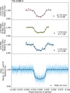 |
Fig. 4 Phase-folded light curves of TOI-3288 from TESS-SPOC, QLP, and LCO (SSO, SAAO, and CTIO). If a dilution factor was fitted, it is indicated in the legend of each subpanel. Markers with black edges represent data binned per 10 or 15 minutes, as is noted in the legend. |
6.1 TOI-3288
TOI-3288 b is a 2.11 ± 0.08 MJup gas giant planet transiting a K 9 V star every 1.4 days. With a radius of 1.00 ± 0.03 RJup and a equilibrium temperature of 1059 ± 20 K, it is a relatively massive hot Jupiter. Fig. 4 shows the photometric data with the derived median posterior model.
Fig. 5 shows the post-processed HARPS and NIRPS RVs. Separately, HARPS finds K = 486 ± 33 m s−1, and NIRPS finds K = 532 ± 33 m s−1, consistent within 1σ. Combined, the two instruments give K = 511 ± 19 m s−1. Table 4 presents the joint fit results.
6.2 TOI-4666
TOI-4666 is a M2.5 main-sequence star hosting a 0.70 ± 0.06 MJup giant planet. Despite its short orbital period of 2.9 days, the planet’s equilibrium temperature is only 713 ± 14 K due to the low insolation flux (54 ± 3 S⊕) received from its cool host, placing it outside the typical hot Jupiter range.
Figs. 6 and 7 show the photometry data with the median posterior model. The orbital period is refined with greater precision by the additional transits observed by ExTrA. The ExTrA data show residual instrumental systematics, as the linear regression airmass correction does not fully account for the deviations from the out-of-transit baseline. However, no GP was included in the joint fit to avoid computational cost. Each transit and telescope is treated as a separate instrument with distinct systematics, except for the limb-darkening coefficient, which is shared for all three telescopes.
Fig. 8 shows the HARPS and NIRPS RVs. When fitted separately, HARPS finds K = 114 ± 22 m s−1 and NIRPS K = 162 ± 21 m s−1, consistent within 1.6 σ, indicating a relatively good agreement between the optical and nIR. The joint fit results in K = ![Mathematical equation: $\[144_{-12}^{+11}\]$](/articles/aa/full_html/2026/03/aa57656-25/aa57656-25-eq22.png) m s−1.
m s−1.
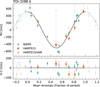 |
Fig. 5 Night-binned RVs of TOI-3288 with the Juliet orbital solution overplotted as a black line. The residuals have an RMS of ~65 m s−1. The RVs have been cleaned on telluric contamination. The RVs from before the post-processing steps are shown as grey squares, with dotted lines indicating the difference from the corrected values. |
6.3 Eccentricity
In our analysis, we adopted fixed values for the orbital eccentricity and argument of periastron (e = 0 and ω = 90°). Allowing these parameters to vary yields 1 σ upper limits on the eccentricity of 0.03 for TOI-3288 b and 0.10 for TOI-4666 b, while ω remains unconstrained. A model comparison using the logevidence from our Juliet fits indicates that both planets are best described by e = 0 solutions. Specifically, when fitting only the RV data, the log-evidence for TOI-3288 is −11.118 ± 0.435 assuming a circular orbit, and −13.930 ± 0.456 including eccentricity. For TOI-4666 a circular orbit has a log-evidence of 6.218 ± 0.438, decreasing to 4.585 ± 0.431 with eccentricity. This is consistent with close-in giants (P ≲ 3 d) rapidly circularising due to strong tidal dissipation (Hut 1981).
7 Discussion
With NIRPS, we characterise two gas giants orbiting low-mass stars: TOI-3288 b and TOI-4666 b. As is shown in Fig. 9, these companions occupy a relatively sparse region of the known transiting exoplanets. Through the NIRPS-GTO sub-programme, we are helping to fill in the exoplanet population around low-mass stars, using NIRPS’s ability to observe faint M dwarfs. In the following subsections, we discuss the age, interior structure, binarity, metallicity, and atmospheric properties of these planets, as well as the effect of the remnant telluric contamination correction on the RVs.
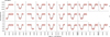 |
Fig. 6 Normalised flux versus time of TOI-4666 transits observed with ExTrA, shown per telescope. The Juliet fit is represented by the black line, and the black markers with black outlines represent data binned in 30-minute intervals. |
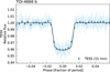 |
Fig. 7 Phase-folded TESS light curve of TOI-4666, with the Juliet fit shown as a black line. Markers with black edges indicate 15-minute binned data. |
7.1 Age
If the periodicity detected in the TESS light curves is not due to instrumental artefacts, the implied stellar rotation periods are relatively short for these types of stars (Barnes 2003, 2007). Such short rotation periods could indicate that they are young. TOI-3288 has a 24% probability of being associated with the tidal tail of UPK612, which has an estimated age of ~100 Myr (Kos 2024). TOI-4666, however, is not known to be associated with any cluster. Using the stellar parameters (Teff, [Fe/H], log g, Lbol, and ω; see Table 3), we estimated ages from PARSEC isochrones (Bressan et al. 2012) via the PARAM1.5 web interface9. We find ages of ![Mathematical equation: $\[590_{-200}^{+300}\]$](/articles/aa/full_html/2026/03/aa57656-25/aa57656-25-eq23.png) Myr for TOI-3288 and 80 ± 6 Myr for TOI-4666. Since TOI-4666 is not affiliated with a young cluster, there is no other strong evidence that it is this young.
Myr for TOI-3288 and 80 ± 6 Myr for TOI-4666. Since TOI-4666 is not affiliated with a young cluster, there is no other strong evidence that it is this young.
7.2 Interior
We used the planetary evolution code completo (Mordasini et al. 2012b) to estimate the heavy element mass of both planets. The planet is modelled with a core of iron and silicates with a mass up to 10 M⊕, an envelope along with a semi-grey atmospheric model. The envelope contains hydrogen and helium modelled with the equation of state (EoS) from Chabrier & Debras (2021), and the heavy elements are modelled as water with the EoS AQUA from Haldemann et al. (2020). According to the empirical formulas of Sestovic et al. (2018), TOI-3288 b and TOI-4666 b are not inflated, as neither exceeds the threshold in incident flux for its planetary mass. Given this relatively low irradiation, no inflation parameters are included in the modelling.
We built a grid of evolution models coupled with a Bayesian inference scheme to retrieve the heavy element content compatible with the observed planetary parameters. For TOI-3288 b, we used a normal prior on the stellar age centred on 0.6 Gyr. We find a heavy element fraction in the envelope of Z = 0.28 ± 0.04 and a total heavy element mass of 190 ± 25 M⊕. For TOI-4666, using a normal prior around 300 Myr, we find a heavy element fraction in the envelope of Z = 0.12 ± 0.06 and a total heavy element mass of 31 ± 14 M⊕. We note that at young ages the interior models may be sensitive to the initial conditions and that different interior models may lead to variations in the derived heavy element content.
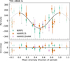 |
Fig. 8 Night-binned RVs of TOI-4666 with the Juliet orbital solution overplotted. The residuals have an RMS of ~75 m s−1. The RVs before the post-processing steps are shown as grey squares, with dotted lines indicating the difference from the corrected values. |
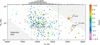 |
Fig. 9 TOI-3288 b and TOI-4666 b (red encircled) compared to known transiting exoplanets from the PlanetS catalogue (Otegi et al. 2020; Parc et al. 2024, updated August 2025). Marker colours show stellar metallicity, with grey for stars of unknown metallicity. Stellar markers indicate planetary companions in binary systems. Circles are single stars. The vertical grey line marks 4600 K. The relative occurrence of the gas giants with masses between 0.1 and 13 MJup is shown as a histogram at the top. Our two mass characterisations contribute to a rare population of exoplanets. |
7.3 Binarity
Many of the lower-mass giants around low-mass stars are in binaries, hinting that, besides metallicity, binarity might also enhance giant planet formation. In Fig. 9 stellar-shaped markers indicate companions in binary systems. We examined their distribution to assess whether binarity affects formation, and found that 17% of stars hosting giant planets with Teff ≥ 4600 K are in binary systems, compared to 24% for Teff < 4600 K and 39% for Teff < 3890 K.
TOI-3288 is part of a wide binary system with an angular separation of approximately 2.3″, corresponding to a physical separation of ~435 AU. The presence of a gravitationally bound companion was confirmed using astrometric data from Gaia DR3, which reveals consistent parallaxes and proper motions between the two stars (Mugrauer et al. 2023). Assuming the two components have the same age and are both in the main sequence, the G-band magnitude of 17.2 mag for the stellar companion translates into a spectral type close to M4V according to the tabulated relations of Pecaut & Mamajek (2013).
The formation of giant planets around low-mass stars presents a challenge to standard core accretion models, which predict limited planetary growth due to the reduced mass reservoir in their protoplanetary disc. Fabrycky & Tremaine (2007) have shown that wide binary systems (>100 AU) may facilitate planet migration through mechanisms such as Kozai-Lidov cycles and dynamical interactions. Alternatively, simulations suggest that stellar companions at separations of a few hundred AU can trigger gravitational disc instability, leading to the formation of massive planets and brown dwarfs (Cadman et al. 2022).
Observational studies have shown that the most massive short-period giant planets are preferentially found in multiple star systems (Zucker & Mazeh 2002; Eggenberger et al. 2004; Desidera & Barbieri 2007; Fontanive & Bardalez Gagliuffi 2021). Ngo et al. (2016) have shown that the occurrence rate of hot Jupiters is 2.9 times larger for binaries with separation in the range of 50–2000 AU than for field stars. Similarly, Eeles-Nolle & Armstrong (2025) found elevated stellar multiplicity rates for hot Jupiter hosts.
The presence of a stellar companion may have altered the formation, migration, and evolution of TOI-3288 b, through gravitational perturbations affecting the protoplanetary disc. Given its physical separation (<1000 AU), the stellar companion to TOI-3288 falls within the regime in which migration and dynamical interactions may be at play. While the companion is unlikely to have truncated the protoplanetary disc, it may have influenced the formation and evolution of the planet and contributed to orbital evolution processes.
7.4 Metallicity
Metal-rich stars are more likely to host giant exoplanets, as is described by the planet-metallicity correlation for FGK stars (Ida & Lin 2004; Santos et al. 2004; Fischer & Valenti 2005) and for M dwarfs (Gan et al. 2025). Here, we report an additional tentative trend in the observations: more massive gas giants are hosted by more metal-rich stars.
There are regions in Fig. 9 where few giant planets are found, which we have defined by eye and shaded in grey to emphasise the observed scarcity. The shaded area for Teff ≳ 6000 K reflects detection biases, while the second region highlights the apparent upper envelope of massive gas giants around low-mass stars. Although low-mass giants are challenging to characterise around low-mass stars, massive gas giants should be easily detectable. Their paucity therefore suggests that such planets rarely form around low-mass stars.
When comparing the giants around low-mass stars (Teff < 4600 K) inside this region to those outside, a tentative trend emerges: the giants within the scarcely populated region tend to orbit more metal-rich host stars (mean metallicity ~0.44 dex) than those outside (~0.16 dex). This aligns with theoretical expectations (Thommes et al. 2008; Mordasini et al. 2012a) whereby low-mass stars are thought to host less massive protoplanetary discs, but high metallicity can compensate for a lower disc mass (Vorobyov & Basu 2008; Alibert et al. 2011; Hobson et al. 2018), and vice versa.
7.5 NIRPS’ faint end
At the faint end of NIRPS, we are more limited by telluric contamination than on the bright side. The technique proposed in Sect. 5 reduces remnant contamination. Using an RV-only Juliet fit to the uncorrected and corrected RVs, the RMS of the residuals for TOI-3288 decreases from 373 m s−1 to 92 m s−1, and for TOI-4666 from 135 m s−1 to 70 m s−1. With this relatively straightforward approach, we can ensure that no telluric contamination influences the remaining RVs. Any remaining scatter is introduced by the low S/N of our observations. The remaining RMS is slightly larger than the median photon noise of the observations, which could suggest underestimated errors. This underestimation is not due to the BERV-window exclusion. While excluding this region reduces information, and thus increases the errors, the OH-dominated region was already introducing noise, so the effect is not expected to be significant. Instead, the excess RMS could stem from stellar activity, as was expected for K 9 V and M 2.5 V hosts, especially if the estimated rotation periods and ages are reliable. We do not attribute this remaining signal to an additional planet, as the S/N in both the NIRPS and HARPS data is too low to draw conclusions.
7.6 Atmospheric characterisation
The transiting nature and short orbital periods of these planets make them possible targets for atmospheric characterisation. We assessed their feasibility using the transmission and emission spectroscopy metrics (TSM and ESM) defined by Kempton et al. (2018). Both planets show potential for atmospheric followup, although they may be less favourable than some well-known hot Jupiters. TOI-3288 b has an ESM of 104, a TSM of 30, and a scale height of 117 km. TOI-4666 b has an ESM of 77, a TSM of 109, and a scale height of 309 km. The latter may be particularly interesting, as it orbits an early M dwarf and is classified as a warm Jupiter. However, their magnitudes (V ~ 15, J ~ 12, H ~ 11) may limit the availability of facilities for high-resolution spectroscopic follow-up. While warm Jupiters are typically harder to study, the ELT will enable this. The upcoming ELT spectrographs ANDES and METIS aim to characterise smaller and warmer planets than the typical ultra-hot Jupiters. As giant planets around M dwarfs are rare, and only a select number have favourable conditions for atmospheric follow-up, TOI-3288 b and TOI-4666 b stand out as valuable opportunities to probe giant-planet atmospheres in the low-mass-star regime.
8 Conclusions
In this work we confirm and characterise new gas giants transiting low-mass stars identified by TESS. We post-processed the NIRPS DRS spectra to further mitigate telluric contamination, excluding a window centred on the BERV from the Gaussian fit when determining RVs from a CCF. From these cleaned RVs, we find that TOI-3288 b is a dense hot Jupiter in a system with a stellar companion, while TOI-4666 b is a low-density warm Jupiter, likely with a puffy atmosphere. Their unique properties make them valuable targets for exploring giant planet formation around low-mass stars, where binarity and metallicity may play key roles. The NIRPS-GTO sub-programme will continue to characterise transiting gas giants, in parallel with CORALIE, which focuses on late K dwarfs (Frensch et al. 2025), to further explore the apparent decline of massive gas giants around low-mass stars.
Data availability
Tables H.1, H.2, I.1 and I.2 are available at the CDS via https://cdsarc.cds.unistra.fr/viz-bin/cat/J/A+A/707/A73.
Acknowledgements
Some of the observations in this paper made use of the High-Resolution Imaging instrument Zorro and were obtained under Gemini LLP Proposal Number: GN/S-2021A-LP-105. Zorro was funded by the NASA Exoplanet Exploration Program and built at the NASA Ames Research Center by Steve B. Howell, Nic Scott, Elliott P. Horch, and Emmett Quigley. Zorro was mounted on the Gemini South telescope of the international Gemini Observatory, a program of NSF’s OIR Lab, which is managed by the Association of Universities for Research in Astronomy (AURA) under a cooperative agreement with the National Science Foundation. on behalf of the Gemini partnership: the National Science Foundation (United States), National Research Council (Canada), Agencia Nacional de Investigación y Desarrollo (Chile), Ministerio de Ciencia, Tecnología e Innovación (Argentina), Ministério da Ciência, Tecnologia, Inovações e Comunicações (Brazil), and Korea Astronomy and Space Science Institute (Republic of Korea). AL acknowledges support from the Fonds de recherche du Québec (FRQ) – Secteur Nature et technologies under file #349961. AL, LMa, RA, BB, CC, RD, ÉA & FBa acknowledge the financial support of the FRQ-NT through the Centre de recherche en astrophysique du Québec as well as the support from the Trottier Family Foundation and the Trottier Institute for Research on Exoplanets. The Board of Observational and Instrumental Astronomy (NAOS) at the Federal University of Rio Grande do Norte’s research activities are supported by continuous grants from the Brazilian funding agency CNPq. This study was partially funded by the Coordenação de Aperfeiçoamento de Pessoal de Nível Superior—Brasil (CAPES) — Finance Code 001 and the CAPES-Print program. 0 XDu acknowledges the support from the European Research Council (ERC) under the European Union’s Horizon 2020 research and innovation programme (grant agreement SCORE No. 851555) and from the Swiss National Science Foundation under the grant SPECTRE (No. 200021_215200). This work has been carried out within the framework of the NCCR PlanetS supported by the Swiss National Science Foundation under grants 51NF40_182901 and 51NF40_205606. LMa, RD, ÉA and FBa acknowledges support from Canada Foundation for Innovation (CFI) program, the Université de Montréal and Université Laval, the Canada Economic Development (CED) program and the Ministere of Economy, Innovation and Energy (MEIE). XB, XDe & TF acknowledge funding from the French ANR under contract number ANR24CE493397 (ORVET), and the French National Research Agency in the framework of the Investissements d’Avenir program (ANR-15-IDEX-02), through the funding of the “Origin of Life” project of the Grenoble-Alpes University. ED-M, JGd, NCS, SCB and EC acknowledge the support from FCT – Fundação para a Ciência e a Tecnologia through national funds by these grants: UIDB/04434/2020, UIDP/04434/2020. ED-M further acknowledges the support from FCT through Stimulus FCT contract 2021.01294.CEECIND. ED-M acknowledges the support by the Ramón y Cajal contract RyC2022-035854-I funded by MICIU/AEI/10.13039/501100011033 and by ESF+. NN, JIGH, ASM and RR acknowledge financial support from the Spanish Ministry of Science, Innovation and Universities (MICIU) projects PID2020-117493GB-I00 and PID2023-149982NB-I00. NN acknowledges financial support by Light Bridges S.L, Las Palmas de Gran Canaria. NN acknowledges funding from Light Bridges for the Doctoral Thesis “Habitable Earth-like planets with ESPRESSO and NIRPS”, in cooperation with the Instituto de Astrofísica de Canarias, and the use of Indefeasible Computer Rights (ICR) being commissioned at the ASTRO POC project in the Island of Tenerife, Canary Islands (Spain). The ICR-ASTRONOMY used for his research was provided by Light Bridges in cooperation with Hewlett Packard Enterprise (HPE). KAM acknowledges support from the Swiss National Science Foundation (SNSF) under the Postdoc Mobility grant P500PT_230225. RA acknowledges the Swiss National Science Foundation (SNSF) support under the Post-Doc Mobility grant P500PT_222212 and the support of the Institut Trottier de Recherche sur les Exoplanètes (IREx). We acknowledge funding from the European Research Council under the ERC Grant Agreement no. 337591-ExTrA. JRM acknowledges CNPq research fellowships (Grant No. 308928/2019-9). Co-funded by the European Union (ERC, FIERCE, 101052347). Views and opinions expressed are however those of the author(s) only and do not necessarily reflect those of the European Union or the European Research Council. Neither the European Union nor the granting authority can be held responsible for them. GAW is supported by a Discovery Grant from the Natural Sciences and Engineering Research Council (NSERC) of Canada. SCB acknowledges the support from Fundação para a Ciência e Tecnologia (FCT) in the form of a work contract through the Scientific Employment Incentive program with reference 2023.06687.CEECIND and DOI 10.54499/2023.06687.CEECIND/CP2839/CT0002. NBC acknowledges support from an NSERC Discovery Grant, a Canada Research Chair, and an Arthur B. McDonald Fellowship, and thanks the Trottier Space Institute for its financial support and dynamic intellectual environment. DE acknowledge support from the Swiss National Science Foundation for project 200021_200726. The authors acknowledge the financial support of the SNSF. ICL acknowledges CNPq research fellowships (Grant No. 313103/2022-4). BLCM acknowledge CAPES postdoctoral fellowships. BLCM acknowledges CNPq research fellowships (Grant No. 305804/2022-7). CMo acknowledges the funding from the Swiss National Science Foundation under grant 200021_204847 “PlanetsInTime”. CP acknowledges support from the NSERC Vanier scholarship, and the Trottier Family Foundation. CP also acknowledges support from the E. Margaret Burbidge Prize Postdoctoral Fellowship from the Brinson Foundation.
References
- Alibert, Y., Mordasini, C., & Benz, W. 2011, A&A, 526, A63 [NASA ADS] [CrossRef] [EDP Sciences] [Google Scholar]
- Allart, R., Lovis, C., Faria, J., et al. 2022, A&A, 666, A196 [NASA ADS] [CrossRef] [EDP Sciences] [Google Scholar]
- Antoniadis-Karnavas, A., Sousa, S. G., Delgado-Mena, E., et al. 2020, A&A, 636, A9 [NASA ADS] [CrossRef] [EDP Sciences] [Google Scholar]
- Antoniadis-Karnavas, A., Sousa, S. G., Delgado-Mena, E., Santos, N. C., & Andreasen, D. T. 2024, A&A, 690, A58 [NASA ADS] [CrossRef] [EDP Sciences] [Google Scholar]
- Artigau, E., Cadieux, C., Cook, N. J., et al. 2022, AJ, 164, 84 [NASA ADS] [CrossRef] [Google Scholar]
- Artigau, E., Bouchy, F., Doyon, R., et al. 2024, in Ground-based and Airborne Instrumentation for Astronomy X, eds. J. R. Vernet, J. J. Bryant, & K. Motohara (Yokohama, Japan: SPIE), 12 [Google Scholar]
- Baranne, A., Queloz, D., Mayor, M., et al. 1996, A&AS, 119, 373 [Google Scholar]
- Barnes, S. A. 2003, ApJ, 586, 464 [Google Scholar]
- Barnes, S. A. 2007, ApJ, 669, 1167 [Google Scholar]
- Blind, N. 2022, in Ground-based and Airborne Instrumentation for Astronomy IX, eds. C. J. Evans, J. J. Bryant, & K. Motohara (Montréal, Canada: SPIE), 168 [Google Scholar]
- Bonfils, X., Delfosse, X., Udry, S., et al. 2013, A&A, 549, A109 [NASA ADS] [CrossRef] [EDP Sciences] [Google Scholar]
- Bonfils, X., Almenara, J. M., Jocou, L., et al. 2015, SPIE Conf. Ser., 9605, 96051L [NASA ADS] [Google Scholar]
- Bouchy, F., Doyon, R., Pepe, F., et al. 2025, A&A, 700, A10 [NASA ADS] [CrossRef] [EDP Sciences] [Google Scholar]
- Bressan, A., Marigo, P., Girardi, L., et al. 2012, MNRAS, 427, 127 [NASA ADS] [CrossRef] [Google Scholar]
- Brown, T. M., Baliber, N., Bianco, F. B., et al. 2013, PASP, 125, 1031 [Google Scholar]
- Bryant, E. M., Bayliss, D., & Van Eylen, V. 2023, MNRAS, 521, 3663 [CrossRef] [Google Scholar]
- Bryant, E. M., Jordán, A., Hartman, J. D., et al. 2025, Nat. Astron., 9, 1031 [Google Scholar]
- Burn, R., Schlecker, M., Mordasini, C., et al. 2021, A&A, 656, A72 [NASA ADS] [CrossRef] [EDP Sciences] [Google Scholar]
- Cabrera, J., Barros, S. C. C., Armstrong, D., et al. 2017, A&A, 606, A75 [NASA ADS] [CrossRef] [EDP Sciences] [Google Scholar]
- Cadman, J., Hall, C., Fontanive, C., & Rice, K. 2022, MNRAS, 511, 457 [NASA ADS] [CrossRef] [Google Scholar]
- Canto Martins, B. L., Gomes, R. L., Messias, Y. S., et al. 2020, ApJS, 250, 20 [NASA ADS] [CrossRef] [Google Scholar]
- Castro-González, A., Díez Alonso, E., Menéndez Blanco, J., et al. 2022, MNRAS, 509, 1075 [Google Scholar]
- Castro-González, A., Lillo-Box, J., Armstrong, D. J., et al. 2024, A&A, 691, A233 [NASA ADS] [CrossRef] [EDP Sciences] [Google Scholar]
- Chabrier, G., & Debras, F. 2021, ApJ, 917, 4 [NASA ADS] [CrossRef] [Google Scholar]
- Ciardi, D. R., Beichman, C. A., Horch, E. P., & Howell, S. B. 2015, ApJ, 805, 16 [NASA ADS] [CrossRef] [Google Scholar]
- Cointepas, M., Almenara, J. M., Bonfils, X., et al. 2021, A&A, 650, A145 [NASA ADS] [CrossRef] [EDP Sciences] [Google Scholar]
- Collins, K. 2019, in American Astronomical Society Meeting Abstracts, 233, 140.05 [NASA ADS] [Google Scholar]
- Collins, K. A., Kielkopf, J. F., Stassun, K. G., & Hessman, F. V. 2017, AJ, 153, 77 [Google Scholar]
- Cook, N. J., Artigau, E., Doyon, R., et al. 2022, PASP, 134, 114509 [NASA ADS] [CrossRef] [Google Scholar]
- Cuntz, M., & Wang, Z. 2018, RNAAS, 2, 19 [NASA ADS] [Google Scholar]
- Cutri, R. M., Skrutskie, M. F., van Dyk, S., et al. 2003, VizieR Online Data Catalog: 2MASS All-Sky Catalog of Point Sources (Cutri+ 2003), VizieR On-line Data Catalog: II/246. Originally published in: University of Massachusetts and Infrared Processing and Analysis Center, (IPAC/California Institute of Technology) [Google Scholar]
- Desidera, S., & Barbieri, M. 2007, A&A, 462, 345 [NASA ADS] [CrossRef] [EDP Sciences] [Google Scholar]
- Dumusque, X. 2018, A&A, 620, A47 [NASA ADS] [CrossRef] [EDP Sciences] [Google Scholar]
- Eeles-Nolle, F., & Armstrong, D. J. 2025, MNRAS, 541, 1419 [Google Scholar]
- Eggenberger, A., Udry, S., Mayor, M., et al. 2004, in Astronomical Society of the Pacific Conference Series, 321, Extrasolar Planets: Today and Tomorrow, eds. J. Beaulieu, A. Lecavelier Des Etangs, & C. Terquem, 93 [Google Scholar]
- ESA. 1997, ESA Special Publication, 1200 [Google Scholar]
- Espinoza, N., Kossakowski, D., & Brahm, R. 2019, MNRAS, 490, 2262 [Google Scholar]
- Fabrycky, D., & Tremaine, S. 2007, ApJ, 669, 1298 [NASA ADS] [CrossRef] [Google Scholar]
- Faria, J. P. 2025, https://doi.org/10.5281/zenodo.17287963 [Google Scholar]
- Fellgett, P. 1953, J. Opt. Soc. Am., 43, 271 [NASA ADS] [CrossRef] [Google Scholar]
- Fischer, D. A., & Valenti, J. 2005, ApJ, 622, 1102 [NASA ADS] [CrossRef] [Google Scholar]
- Fontanive, C., & Bardalez Gagliuffi, D. 2021, Front. Astron. Space Sci., 8, 16 [NASA ADS] [CrossRef] [Google Scholar]
- Foreman-Mackey, D. 2016, J. Open Source Softw., 1, 24 [Google Scholar]
- Frensch, Y., Bouchy, F., Blind, N., et al. 2022, in Ground-based and Airborne Instrumentation for Astronomy IX, eds. C. J. Evans, J. J. Bryant, & K. Motohara (Montréal, Canada: SPIE), 189 [Google Scholar]
- Frensch, Y. G. C., Bouchy, F., Lo Curto, G., et al. 2025, A&A, 700, A118 [NASA ADS] [CrossRef] [EDP Sciences] [Google Scholar]
- Furlan, E., & Howell, S. B. 2017, AJ, 154, 66 [NASA ADS] [CrossRef] [Google Scholar]
- Furlan, E., & Howell, S. B. 2020, ApJ, 898, 47 [NASA ADS] [CrossRef] [Google Scholar]
- Gaia Collaboration (Vallenari, A., et al.) 2023, A&A, 674, A1 [NASA ADS] [CrossRef] [EDP Sciences] [Google Scholar]
- Gan, T., Wang, S. X., Wang, S., et al. 2023, AJ, 165, 17 [NASA ADS] [CrossRef] [Google Scholar]
- Gan, T., Theissen, C. A., Wang, S. X., Burgasser, A. J., & Mao, S. 2025, ApJS, 276, 47 [Google Scholar]
- Gordon, I. E., Rothman, L. S., Hargreaves, R. J., et al. 2022, J. Quant. Spec. Radiat. Transf., 277, 107949 [NASA ADS] [CrossRef] [Google Scholar]
- Grossmann, A., & Morlet, J. 1984, SIAM J. Math. Anal., 15, 723 [Google Scholar]
- Guerrero, N. M., Seager, S., Huang, C. X., et al. 2021, ApJS, 254, 39 [NASA ADS] [CrossRef] [Google Scholar]
- Haldemann, J., Alibert, Y., Mordasini, C., & Benz, W. 2020, A&A, 643, A105 [NASA ADS] [CrossRef] [EDP Sciences] [Google Scholar]
- Hobson, M. J., Díaz, R. F., Delfosse, X., et al. 2018, A&A, 618, A103 [NASA ADS] [CrossRef] [EDP Sciences] [Google Scholar]
- Horne, J. H., & Baliunas, S. L. 1986, ApJ, 302, 757 [Google Scholar]
- Howell, S. B., Everett, M. E., Sherry, W., Horch, E., & Ciardi, D. R. 2011, AJ, 142, 19 [Google Scholar]
- Huang, C. X., Quinn, S. N., Vanderburg, A., et al. 2020a, ApJ, 892, L7 [Google Scholar]
- Huang, C. X., Vanderburg, A., Pál, A., et al. 2020b, Res. Notes AAS, 4, 204 [Google Scholar]
- Husser, T.-O., Wende-von Berg, S., Dreizler, S., et al. 2013, A&A, 553, A6 [NASA ADS] [CrossRef] [EDP Sciences] [Google Scholar]
- Hut, P. 1981, A&A, 99, 126 [NASA ADS] [Google Scholar]
- Ida, S., & Lin, D. N. C. 2004, ApJ, 616, 567 [NASA ADS] [CrossRef] [Google Scholar]
- Ida, S., & Lin, D. N. C. 2005, ApJ, 626, 1045 [NASA ADS] [CrossRef] [Google Scholar]
- Iuzzolino, M., Tozzi, A., Sanna, N., Zangrilli, L., & Oliva, E. 2014, SPIE Conf. Ser., 9147, 914766 [Google Scholar]
- Jahandar, F., Doyon, R., Artigau, E., et al. 2024, ApJ, 966, 56 [CrossRef] [Google Scholar]
- Jahandar, F., Doyon, R., Artigau, E., et al. 2025, ApJ, 978, 154 [Google Scholar]
- Jenkins, J. M. 2002, ApJ, 575, 493 [Google Scholar]
- Jenkins, J. M., Chandrasekaran, H., McCauliff, S. D., et al. 2010, SPIE Conf. Ser., 7740, 77400D [Google Scholar]
- Jenkins, J. M., Tenenbaum, P., Seader, S., et al. 2020, Kepler Data Processing Handbook: Transiting Planet Search, Tech. rep. [Google Scholar]
- Jensen, E. 2013, Astrophysics Source Code Library [record ascl:1306.007] [Google Scholar]
- Kempton, E. M.-R., Bean, J. L., Louie, D. R., et al. 2018, PASP, 130, 114401 [CrossRef] [Google Scholar]
- Khata, D., Mondal, S., Das, R., & Baug, T. 2021, MNRAS, 507, 1869 [NASA ADS] [CrossRef] [Google Scholar]
- Kinemuchi, K., Barclay, T., Fanelli, M., et al. 2012, PASP, 124, 963 [Google Scholar]
- Kipping, D. M. 2013, MNRAS, 434, L51 [Google Scholar]
- Kipping, D. M. 2014, MNRAS, 440, 2164 [CrossRef] [Google Scholar]
- Kochanek, C. S., Shappee, B. J., Stanek, K. Z., et al. 2017, PASP, 129, 104502 [Google Scholar]
- Kos, J. 2024, A&A, 691, A28 [NASA ADS] [CrossRef] [EDP Sciences] [Google Scholar]
- Kunimoto, M., & Daylan, T. 2021, in Posters from the TESS Science Conference II (TSC2), 62 [Google Scholar]
- Kunimoto, M., Daylan, T., Guerrero, N., et al. 2022, ApJS, 259, 33 [NASA ADS] [CrossRef] [Google Scholar]
- Laughlin, G., Bodenheimer, P., & Adams, F. C. 2004, ApJ, 612, L73 [NASA ADS] [CrossRef] [Google Scholar]
- Li, J., Tenenbaum, P., Twicken, J. D., et al. 2019, PASP, 131, 024506 [NASA ADS] [CrossRef] [Google Scholar]
- Lightkurve Collaboration (Cardoso, J. V. d. M., et al.) 2018, Astrophysics Source Code Library [record ascl:1812.013] [Google Scholar]
- Mann, A. W., Feiden, G. A., Gaidos, E., Boyajian, T., & Braun, K. V. 2015, ApJ, 804, 64 [CrossRef] [Google Scholar]
- Mann, A. W., Dupuy, T., Kraus, A. L., et al. 2019, ApJ, 871, 63 [Google Scholar]
- Mann, A. W., Wood, M. L., Schmidt, S. P., et al. 2022, AJ, 163, 156 [NASA ADS] [CrossRef] [Google Scholar]
- Marcy, G. W., Butler, R. P., Vogt, S. S., Fischer, D., & Lissauer, J. J. 1998, ApJ, 505, L147 [Google Scholar]
- Mayor, M., Pepe, F., Queloz, D., et al. 2003, The Messenger, 114, 20 [NASA ADS] [Google Scholar]
- McCully, C., Volgenau, N. H., Harbeck, D.-R., et al. 2018, SPIE Conf. Ser., 10707, 107070K [Google Scholar]
- Mignon, L., Delfosse, X., Meunier, N., et al. 2025, A&A, 700, A146 [NASA ADS] [CrossRef] [EDP Sciences] [Google Scholar]
- Morales, J. C., Mustill, A. J., Ribas, I., et al. 2019, Science, 365, 1441 [Google Scholar]
- Mordasini, C., Alibert, Y., Benz, W., Klahr, H., & Henning, T. 2012a, A&A, 541, A97 [NASA ADS] [CrossRef] [EDP Sciences] [Google Scholar]
- Mordasini, C., Alibert, Y., Klahr, H., & Henning, T. 2012b, A&A, 547, A111 [NASA ADS] [CrossRef] [EDP Sciences] [Google Scholar]
- Mugrauer, M., Rück, J., & Michel, K. U. 2023, Astron. Nachr., 344, e20230055 [Google Scholar]
- Neves, V., Bonfils, X., Santos, N. C., et al. 2012, A&A, 538, A25 [NASA ADS] [CrossRef] [EDP Sciences] [Google Scholar]
- Ngo, H., Knutson, H. A., Hinkley, S., et al. 2016, ApJ, 827, 8 [Google Scholar]
- Otegi, J. F., Bouchy, F., & Helled, R. 2020, A&A, 634, A43 [NASA ADS] [CrossRef] [EDP Sciences] [Google Scholar]
- Paegert, M., Stassun, K. G., Collins, K. A., et al. 2021, TESS Input Catalog versions 8.1 and 8.2: Phantoms in the 8.0 Catalog and How to Handle Them [Google Scholar]
- Parc, L., Bouchy, F., Venturini, J., Dorn, C., & Helled, R. 2024, A&A, 688, A59 [NASA ADS] [CrossRef] [EDP Sciences] [Google Scholar]
- Parc, L., Bouchy, F., Cook, N. J., et al. 2025, A&A, 702, A138 [NASA ADS] [CrossRef] [EDP Sciences] [Google Scholar]
- Parviainen, H., Palle, E., Zapatero-Osorio, M. R., et al. 2021, A&A, 645, A16 [NASA ADS] [CrossRef] [EDP Sciences] [Google Scholar]
- Pass, E. K., Winters, J. G., Charbonneau, D., et al. 2023, AJ, 166, 11 [NASA ADS] [CrossRef] [Google Scholar]
- Pecaut, M. J., & Mamajek, E. E. 2013, ApJS, 208, 9 [Google Scholar]
- Pepe, F., Cristiani, S., Rebolo, R., et al. 2021, A&A, 645, A96 [NASA ADS] [CrossRef] [EDP Sciences] [Google Scholar]
- Pinamonti, M., Sozzetti, A., Maldonado, J., et al. 2022, A&A, 664, A65 [NASA ADS] [CrossRef] [EDP Sciences] [Google Scholar]
- Press, W. H., & Rybicki, G. B. 1989, ApJ, 338, 277 [Google Scholar]
- Prša, A., Harmanec, P., Torres, G., et al. 2016, AJ, 152, 41 [Google Scholar]
- Ribas, I., Reiners, A., Zechmeister, M., et al. 2023, A&A, 670, A139 [NASA ADS] [CrossRef] [EDP Sciences] [Google Scholar]
- Ricker, G. R., Winn, J. N., Vanderspek, R., et al. 2014, J. Astron. Telesc. Instrum. Syst, 1, 014003 [Google Scholar]
- Santos, N. C., Israelian, G., & Mayor, M. 2004, A&A, 415, 1153 [NASA ADS] [CrossRef] [EDP Sciences] [Google Scholar]
- Scargle, J. D. 1982, ApJ, 263, 835 [Google Scholar]
- Schlegel, D. J., Finkbeiner, D. P., & Davis, M. 1998, ApJ, 500, 525 [Google Scholar]
- Scott, N. J., Howell, S. B., Gnilka, C. L., et al. 2021, Front. Astron. Space Sci., 8, 716560 [Google Scholar]
- Seager, S., & Mallen-Ornelas, G. 2003, ApJ, 585, 1038 [Google Scholar]
- Sestovic, M., Demory, B.-O., & Queloz, D. 2018, A&A, 616, A76 [NASA ADS] [CrossRef] [EDP Sciences] [Google Scholar]
- Smith, J. C., Stumpe, M. C., Van Cleve, J. E., et al. 2012, PASP, 124, 1000 [Google Scholar]
- Speagle, J. S. 2020, MNRAS, 493, 3132 [Google Scholar]
- Stassun, K. G., & Torres, G. 2021, ApJ, 907, L33 [NASA ADS] [CrossRef] [Google Scholar]
- Stassun, K. G., Oelkers, R. J., Pepper, J., et al. 2018, AJ, 156, 102 [Google Scholar]
- Stassun, K. G., Oelkers, R. J., Paegert, M., et al. 2019, AJ, 158, 138 [Google Scholar]
- Stumpe, M. C., Smith, J. C., Van Cleve, J. E., et al. 2012, PASP, 124, 985 [Google Scholar]
- Stumpe, M. C., Smith, J. C., Catanzarite, J. H., et al. 2014, PASP, 126, 100 [Google Scholar]
- Suárez Mascareño, A., Artigau, É., Mignon, L., et al. 2025, A&A, 700, A11 [NASA ADS] [CrossRef] [EDP Sciences] [Google Scholar]
- Thommes, E. W., Matsumura, S., & Rasio, F. A. 2008, Science, 321, 814 [NASA ADS] [CrossRef] [Google Scholar]
- Tokovinin, A. 2018, PASP, 130, 035002 [Google Scholar]
- Twicken, J. D., Catanzarite, J. H., Clarke, B. D., et al. 2018, PASP, 130, 064502 [Google Scholar]
- Vorobyov, E. I., & Basu, S. 2008, ApJ, 676, L139 [NASA ADS] [CrossRef] [Google Scholar]
- Wang, S. X., Latouf, N., Plavchan, P., et al. 2022, AJ, 164, 211 [NASA ADS] [CrossRef] [Google Scholar]
- Wildi, F., Bouchy, F., Doyon, R., et al. 2022, in Ground-based and Airborne Instrumentation for Astronomy IX, eds. C. J. Evans, J. J. Bryant, & K. Motohara (Montréal, Canada: SPIE), 51 [Google Scholar]
- Zechmeister, M., & Kürster, M. 2009, A&A, 496, 577 [CrossRef] [EDP Sciences] [Google Scholar]
- Zhan, Z., Günther, M. N., Rappaport, S., et al. 2019, ApJ, 876, 127 [Google Scholar]
- Zucker, S., & Mazeh, T. 2002, ApJ, 568, L113 [NASA ADS] [CrossRef] [Google Scholar]
These values were obtained from Table 5 of Pecaut & Mamajek (2013).
Available at https://github.com/castro-gzlz/TESS-cont
IRAF is distributed by National Optical Astronomy Observatories, operated by the Association of Universities for Research in Astronomy, Inc., under contract with the National Science Foundation, USA.
Appendix A False positives
A.1 TOI-2341 (SB2)
TOI-2341 was early on recognised as a spectroscopic binary and was therefore observed only once. The two components in the CCF are visible in Fig. A.1.
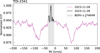 |
Fig. A.1 The normalised NIRPS CCF of the SB2 TOI-2341. The BERV is indicated by a grey shaded area, with limits defined by the FWHM of the stellar components in the CCF. |
A.2 TOI-5295 (Triple system)
TOI-5295 shows a moving component in the NIRPS CCFs computed with an M1 mask (Fig. A.2). The RVs are derived by subtracting the average spectrum from each individual spectrum to suppress the primary signal, and then fitting a Gaussian with iCCF to the residual CCFs. After correcting for the movement of the primary component (negligible at 400 m s−1 compared to 40 km s−1), the RVs of the secondary are consistent with the TESS ephemerides. A simple cosine fit results in a semi-amplitude of K ~ 20 km s−1. The secondary mass is estimated at ~0.4 M⊙, using the mass-luminosity relation of Cuntz & Wang (2018), the primary mass of 0.57 M⊙ from ExoFOP5, and the contrast ratio of the primary and secondary component in the CCFs. The transit of TOI-5295 B is caused by a low-mass (~95 MJup) stellar companion, just above the hydrogen-burning limit, identifying this as a triple star system.
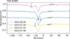 |
Fig. A.2 The normalised NIRPS CCFs of TOI-5295, where the RV variation of the second component is in agreement with the TESS ephemerides. An arbitrary offset has been applied to the NIRPS CCFs to improve visibility. The BERV affected region is indicated in black. |
Appendix B Fast rotators
B.1 TOI-1227
The young star TOI-1227 (11 Myr) was validated as a planet host by Mann et al. (2022) using SOAR (Tokovinin 2018) and LCO photometry, resulting in a planetary radius of 0.85 RJup. As this value falls within our programme’s selection criteria, we attempted NIRPS follow-up. However, the star’s rapid rotation (1.65 ± 0.04 d; Mann et al. 2022) produces significantly broadened CCFs (FWHM ~27 km s−1), and all observations coincided with a BERV crossing, preventing a reliable RV determination. We therefore stopped observations of this target.
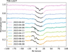 |
Fig. B.1 The normalised NIRPS CCFs of TOI-1227. The BERV affected region is indicated in black. The CCFs are broadened due to the fast stellar rotation. |
B.2 TOI-2455
TOI-2455 has a planetary radius of Rpl = 1.3 RJup, which is relatively large for an M2V host star (Teff = 3553 K; TESS Input Catalog). A significant RV variation would therefore be expected. However, TOI-2455 is a rapid rotator, broadening the CCFs to a FWHM of ~40 km s−1. After one observation, which also coincided with a BERV crossing, the target was stopped.
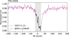 |
Fig. B.2 The normalised NIRPS CCFs of the fast rotating TOI-2455. The BERV affected region is highlighted in grey. |
Appendix C Giant stars
The five TOIs that appear as evolved stars in the HR diagram in Fig. 1 were part of the NIRPS-GTO programme at its start (April 2023). Although transits are reported for these targets, the stellar radii of evolved stars are poorly constrained; consequently, the planetary radii inferred from the transit depths are likewise highly uncertain. We observed TOI-3463 once before recognising it as a giant, and subsequently stopped its followup. For TOI-3209, the Gaia DR3 General Stellar Parametrizer from Photometry (GSP-Phot) library reports a stellar radius of 36.3 R⊙, such that the ~1% transit depth would correspond to a companion of ~3.1 R⊙. For the other stars, no stellar radius is reported by Gaia.
Appendix D SED analysis
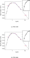 |
Fig. D.1 The SEDs of the presented stars with giant companions. Red symbols represent the observed photometric measurements (as discussed in Section 4.2), and the horizontal bars represent the effective width of the passband. Blue symbols are the model fluxes from the best-fit PHOENIX atmosphere model (black). The insets show the absolute flux-calibrated Gaia spectrophotometry as a grey swathe overlaid on the model (black). |
Appendix E Guiding Frames
Integrated AO guiding frames are available per NIRPS observation. Figure E.1 shows the average frame over all observations for TOI-3288 and TOI-4666. A logarithmic scale is used to enhance the visibility of potential stellar companions. The stellar companion of TOI-3288 is visible at a separation of ~2″. This is the companion discussed in Sect. 7.3, identified as Gaia DR3 6685431748040148992.
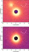 |
Fig. E.1 Integrated NIRPS AO guiding frames for TOI-3288 (top) and TOI-4666 (bottom). The stellar companion Gaia DR3 6685431748040148992 is visible at a separation of ~2″ from TOI-3288. No evidence of a stellar companion is seen for TOI-4666 (Gaia DR3 RUWE = 0.998). The 0.9″ fibre hole partially blocks the stellar light. |
Appendix F Limb darkening and photometric instrumental parameters
Fitted limb darkening parameters for the companions presented in this paper.
Fitted photometric instrumental parameters for the companions presented in this paper.
Fitted photometric instrumental parameters of ExTrA for TOI-4666.
Appendix G Joint modelling priors
Priors for the joint modelling of photometric and RV data.
Appendix H Radial velocities
RVs of TOI-3288.
RVs of TOI-4666.
Appendix I Photometry
TESS photometry of TOI-3288 extracted as described in Section 3.1.
TESS photometry of TOI-4666 extracted as described in Section 3.1.
Appendix J Corner plots
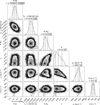 |
Fig. J.1 The corner plot for the TOI-3288 Juliet results. |
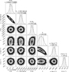 |
Fig. J.2 The corner plot for the TOI-4666 Juliet results. |
Appendix K TESS-cont generated heatmaps
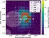 |
Fig. K.1 Sector 13 for TOI-3288. The flux percentage of TOI-3288 is indicated per pixel as an overlay of the TESS FFI. The red box indicates the aperture used to extract the lightcurve, this aperture is 23% contaminated by nearby stars. |
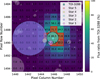 |
Fig. K.2 Sector 27 for TOI-3288. The flux percentage of TOI-3288 is indicated per pixel as an overlay of the TESS FFI. The red box indicates the aperture used to extract the lightcurve, this aperture is 27% contaminated by nearby stars. |
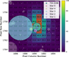 |
Fig. K.3 Sector 67 for TOI-3288. The flux percentage of TOI-3288 is indicated per pixel as an overlay of the TESS FFI. The red box indicates the aperture used to extract the lightcurve, this aperture is 22% contaminated by nearby stars. |
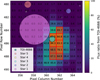 |
Fig. K.4 Sector 31 for TOI-4666. The flux percentage of TOI-4666 is indicated per pixel as an overlay of the TESS FFI. The red box indicates the aperture used to extract the lightcurve, this aperture is 18% contaminated by nearby stars. |
Appendix L ASAS-SN periodograms
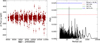 |
Fig. L.1 The g-band ASAS-SN data of TOI-3288 and the corresponding Lomb–Scargle periodogram. |
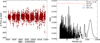 |
Fig. L.2 The g-band ASAS-SN data of TOI-4666 and the corresponding Lomb–Scargle periodogram. |
All Tables
Fitted photometric instrumental parameters for the companions presented in this paper.
All Figures
|
Fig. 1 HR diagram of all Gaia DR3 nearby stars with a parallax of π ≥ 5 mas, using the broad-band G magnitude versus the colour GBP (blue) minus GRP (red). The colours indicate log(g). Stars without a log(g) measurement are shown in grey. The six targets presented in this paper as part of the NIRPS-GTO giants sub-programme are overplotted (outlined black circles), along with five stars identified as giant stars using this method. TOI-3288 and TOI-4666 (outlined black squares), hosting gas giants, are visible on the main sequence. This figure can be generated using Gaia-HR, available at https://github.com/ygcfrensch/Gaia-HR. |
| In the text | |
|
Fig. 2 5 σ magnitude contrast curves as observed by Zorro in both filters as a function of the angular separation out to 1.2″. The insets show the reconstructed speckle images of TOI-3288 with a 1″ scale bar. TOI-3288 was found to have no close companions from the diffraction limit (0.02″) out to 1.2″ to within the magnitude contrast levels achieved. |
| In the text | |
|
Fig. 3 Normalised CCF of TOI-3288. The upper panel shows the full CCF, while the lower panel shows the CCF with the BERV window |
| In the text | |
|
Fig. 4 Phase-folded light curves of TOI-3288 from TESS-SPOC, QLP, and LCO (SSO, SAAO, and CTIO). If a dilution factor was fitted, it is indicated in the legend of each subpanel. Markers with black edges represent data binned per 10 or 15 minutes, as is noted in the legend. |
| In the text | |
|
Fig. 5 Night-binned RVs of TOI-3288 with the Juliet orbital solution overplotted as a black line. The residuals have an RMS of ~65 m s−1. The RVs have been cleaned on telluric contamination. The RVs from before the post-processing steps are shown as grey squares, with dotted lines indicating the difference from the corrected values. |
| In the text | |
|
Fig. 6 Normalised flux versus time of TOI-4666 transits observed with ExTrA, shown per telescope. The Juliet fit is represented by the black line, and the black markers with black outlines represent data binned in 30-minute intervals. |
| In the text | |
|
Fig. 7 Phase-folded TESS light curve of TOI-4666, with the Juliet fit shown as a black line. Markers with black edges indicate 15-minute binned data. |
| In the text | |
|
Fig. 8 Night-binned RVs of TOI-4666 with the Juliet orbital solution overplotted. The residuals have an RMS of ~75 m s−1. The RVs before the post-processing steps are shown as grey squares, with dotted lines indicating the difference from the corrected values. |
| In the text | |
|
Fig. 9 TOI-3288 b and TOI-4666 b (red encircled) compared to known transiting exoplanets from the PlanetS catalogue (Otegi et al. 2020; Parc et al. 2024, updated August 2025). Marker colours show stellar metallicity, with grey for stars of unknown metallicity. Stellar markers indicate planetary companions in binary systems. Circles are single stars. The vertical grey line marks 4600 K. The relative occurrence of the gas giants with masses between 0.1 and 13 MJup is shown as a histogram at the top. Our two mass characterisations contribute to a rare population of exoplanets. |
| In the text | |
|
Fig. A.1 The normalised NIRPS CCF of the SB2 TOI-2341. The BERV is indicated by a grey shaded area, with limits defined by the FWHM of the stellar components in the CCF. |
| In the text | |
|
Fig. A.2 The normalised NIRPS CCFs of TOI-5295, where the RV variation of the second component is in agreement with the TESS ephemerides. An arbitrary offset has been applied to the NIRPS CCFs to improve visibility. The BERV affected region is indicated in black. |
| In the text | |
|
Fig. B.1 The normalised NIRPS CCFs of TOI-1227. The BERV affected region is indicated in black. The CCFs are broadened due to the fast stellar rotation. |
| In the text | |
|
Fig. B.2 The normalised NIRPS CCFs of the fast rotating TOI-2455. The BERV affected region is highlighted in grey. |
| In the text | |
|
Fig. D.1 The SEDs of the presented stars with giant companions. Red symbols represent the observed photometric measurements (as discussed in Section 4.2), and the horizontal bars represent the effective width of the passband. Blue symbols are the model fluxes from the best-fit PHOENIX atmosphere model (black). The insets show the absolute flux-calibrated Gaia spectrophotometry as a grey swathe overlaid on the model (black). |
| In the text | |
|
Fig. E.1 Integrated NIRPS AO guiding frames for TOI-3288 (top) and TOI-4666 (bottom). The stellar companion Gaia DR3 6685431748040148992 is visible at a separation of ~2″ from TOI-3288. No evidence of a stellar companion is seen for TOI-4666 (Gaia DR3 RUWE = 0.998). The 0.9″ fibre hole partially blocks the stellar light. |
| In the text | |
|
Fig. J.1 The corner plot for the TOI-3288 Juliet results. |
| In the text | |
|
Fig. J.2 The corner plot for the TOI-4666 Juliet results. |
| In the text | |
|
Fig. K.1 Sector 13 for TOI-3288. The flux percentage of TOI-3288 is indicated per pixel as an overlay of the TESS FFI. The red box indicates the aperture used to extract the lightcurve, this aperture is 23% contaminated by nearby stars. |
| In the text | |
|
Fig. K.2 Sector 27 for TOI-3288. The flux percentage of TOI-3288 is indicated per pixel as an overlay of the TESS FFI. The red box indicates the aperture used to extract the lightcurve, this aperture is 27% contaminated by nearby stars. |
| In the text | |
|
Fig. K.3 Sector 67 for TOI-3288. The flux percentage of TOI-3288 is indicated per pixel as an overlay of the TESS FFI. The red box indicates the aperture used to extract the lightcurve, this aperture is 22% contaminated by nearby stars. |
| In the text | |
|
Fig. K.4 Sector 31 for TOI-4666. The flux percentage of TOI-4666 is indicated per pixel as an overlay of the TESS FFI. The red box indicates the aperture used to extract the lightcurve, this aperture is 18% contaminated by nearby stars. |
| In the text | |
|
Fig. L.1 The g-band ASAS-SN data of TOI-3288 and the corresponding Lomb–Scargle periodogram. |
| In the text | |
|
Fig. L.2 The g-band ASAS-SN data of TOI-4666 and the corresponding Lomb–Scargle periodogram. |
| In the text | |
Current usage metrics show cumulative count of Article Views (full-text article views including HTML views, PDF and ePub downloads, according to the available data) and Abstracts Views on Vision4Press platform.
Data correspond to usage on the plateform after 2015. The current usage metrics is available 48-96 hours after online publication and is updated daily on week days.
Initial download of the metrics may take a while.