| Issue |
A&A
Volume 707, March 2026
|
|
|---|---|---|
| Article Number | A317 | |
| Number of page(s) | 12 | |
| Section | Celestial mechanics and astrometry | |
| DOI | https://doi.org/10.1051/0004-6361/202557657 | |
| Published online | 24 March 2026 | |
NEOForCE: Near-Earth Objects’ Forecast of Collisional Events
1
LTE, Paris Observatory, univ. PSL, Sorbonne univ., univ. Lille, LNE, CNRS,
61 Av. de l’Observatoire,
75014
Paris,
France
2
Institute of Applied Astronomy, Russian Academy of Sciences,
Kutuzova emb. 10,
St. Petersburg,
Russia
★ Corresponding authors: This email address is being protected from spambots. You need JavaScript enabled to view it.
; This email address is being protected from spambots. You need JavaScript enabled to view it.
; This email address is being protected from spambots. You need JavaScript enabled to view it.
Received:
11
October
2025
Accepted:
22
January
2026
Abstract
Context. Robust impact monitoring of near-Earth objects is an essential task of planetary defense. Current systems such as NASA’s Sentry-II, NEODyS’s CLOMON2, and ESA’s Aegis have been highly successful, but independent approaches are essential to ensure reliability and to cross-validate predictions of possible impacts, probabilities, and paths on Earth.
Aims. We present NEOForCE (Near-Earth Objects’ Forecast of Collisional Events), a new independent monitoring system for asteroid impact prediction. By relying on orbital solutions from DynAstVO at Paris Observatory and using an original methodology for uncertainty propagation, NEOForCE provides an alternative line of verification for future impact assessments and strengthens the overall robustness of planetary defense.
Methods. As other monitoring systems do, NEOForCE samples several thousand so-called “virtual asteroids” from the uncertainty region and integrates their orbits up to 100 years into the future. Instead of searching for close approaches of the virtual asteroids themselves with the Earth, our system looks for times when the Earth comes close to the “realistic” uncertainty regions around them, which are mostly stretched along the osculating ellipses of virtual asteroids. For every virtual asteroid and every possible collision time, we also estimate the maximal impact probability, and only if this value is large enough (>5 × 10⁻⁸) do we continue to the next step. In this second step, we compute how the original asteroid orbit should be slightly modified so that the new trajectory leads to an Earth impact, which allows us to confirm the possible collision and estimate the impact probability.
Results. We tested NEOForCE against NASA’s Sentry-II system on five representative asteroids with a high impact probability and significant number of possible collisions: 2000 SG344, 2005 QK76, 2008 JL3, 2023 DO, and 2008 EX5. NEOForCE successfully recovered almost all of the possible collisions reported by Sentry-II with impact probabilities above 10−7, demonstrating the robustness of our approach. In addition, NEOForCE identified several potential impacts at the 10−7–10−6 level that Sentry-II did not report.
Key words: methods: numerical / celestial mechanics / minor planets, asteroids: general
© The Authors 2026
 Open Access article, published by EDP Sciences, under the terms of the Creative Commons Attribution License (https://creativecommons.org/licenses/by/4.0), which permits unrestricted use, distribution, and reproduction in any medium, provided the original work is properly cited.
This article is published in open access under the Subscribe to Open model. This email address is being protected from spambots. You need JavaScript enabled to view it. to support open access publication.
1 Introduction
Estimating the probability that a particular asteroid can hit the Earth in the foreseeable future is an important task of planetary defense. The orbit of an asteroid in general does not have absolute or infinite precision, and for a newly discovered object the uncertainty of its orbital parameters can be significant. Moreover, this uncertainty increases with time if no additional observations are provided. Therefore, apart from the nominal solution of the orbital parameters (usually computed from the least-squares method), there are other solutions that also represent observations well, sometimes with a similar probability. These sets of orbital parameters are in general called virtual asteroids (VAs; Milani et al. 2000). Some of these VAs can collide with the Earth and some pass by safely, which allows the impact probability to be in a range between 0 and 1.
One of the most natural and general ways to estimate the impact probability is the Monte Carlo approach: sample a large number of VAs from the uncertainty region of orbital parameters according to the probability distribution, propagate their orbit in the future, and lastly derive the impact probability from the fraction of colliding orbits out of all the ones considered in the sample. This approach has many advantages: it does not have additional assumptions, and it also has a direct formula for estimating the uncertainty of the obtained result,  , where PMC is the impact probability and n is the number of considered VAs (Vavilov & Medvedev 2015). However, if the impact probability is small – which is generally the case with NEAs – the number of required VAs to integrate to roughly estimate the impact probability (so that σMC ≲ 0.3PMC) is 10/PMC. Therefore, this approach is impractical as a systematic search for possible impacts with small impact probability values on a large set of of objects.
A much more effective approach is a linear one whereby one assumes that the errors of the orbital parameters at the time of a possible collision, t, are linearly related to the errors at the epoch of observations, t0. In this case, one can integrate only the orbit of the nominal asteroid state vector together with variational equations, deriving the transition matrix and partial derivative matrix of orbital parameters at time t over t0. Using this matrix one can estimate the uncertainty region of the asteroid at time t and assess the impact probability. The first linear method was introduced by Chodas (1993), who also proposed using the target plane (TP) for the impact analysis. In addition to the linear assumption (which can be broken by a close encounter), the important drawback of this approach is that the asteroid must come close to the Earth (enter its sphere of influence at ≈929 000 km), making linearization validity limited. Vavilov & Medvedev (2015) proposed the use of a special curvilinear coordinate system related to the asteroid’s osculating orbit to overcome this limitation. This allows us to calculate satisfactorily accurate probabilities of an asteroid collision with the Earth, even if the distance between the Earth and the nominal asteroid at time t exceeds 1 au. Later Vavilov (2020) improved this approach and called it the partial banana mapping (PBM) method. The method constructs the curvilinear uncertainty region of an asteroid then finds the part of this region that is closest to the Earth and maps it to the TP. However, the linear relation between the errors of orbital parameters is a very important assumption and is limiting the usage of linear methods to the situation when the two-body formalism is not significantly violated.
A better compromise between linear methods and a full Monte Carlo approach was introduced by Milani (1999) as a concept of a line of variations (LOV). Instead of sampling the full multi-dimensional phase-space, the LOV reduces the problem to a single dimension that follows the direction where uncertainties and nonlinear effects are strongest (Milani et al. 2002, 2005a,b). By distributing VAs along this line and interpolating between them, one can efficiently identify possible impacting solutions and trace distinct dynamical pathways. This approach makes it possible to detect even very small impact probabilities, while keeping the computational effort manageable. Because of these advantages, operational monitoring systems at NASA, Sentry1, CLOMON22 (operated by NEODyS), and ESA’s Aegis3 were all built upon the LOV technique. Recently, NASA introduced the Sentry-II system (Roa et al. 2021), which samples the full confidence region rather than restricting itself to LOV. Potential impacts are then confirmed by adding an impact pseudo-observation and refitting the orbit to match the data. These methods require several thousand VA orbits to integrate for the first search of close encounters only, but can detect possible impacts with probabilities on the order of 10−7 while being much more efficient than the Monte Carlo one.
Vavilov & Hestroffer (2025) introduced a semi-linear method of impact probability estimation, as an extension of the linear PBM method (Vavilov 2020) built in previous work. This extension (called impactor PBM or improved PBM: IPBM) consists of a direct search for a state vector at the epoch of observations, t0, which leads to a close encounter at the time of a possible collision, t. This method requires several orbits to be integrated, but still much fewer than is required by Sentry of CLOMON2 systems. The method has a moderate limitation in the way that the asteroid position’s uncertainty should not exceed the whole orbit: if a VA that collides with the Earth makes a different number of revolutions around the Sun than the nominal one, this collision cannot be found. This naturally puts a threshold on the impact probability that can be more or less guaranteed to be found (order of 10−5). This method successfully fills the gap between restricted but very efficient linear methods and robust nonlinear methods that require the propagation of several thousand orbits.
In this work, we want to extend the applicability of this semi-linear method so that we can find a possible collision with smaller impact probability values. We call our monitoring system Near-Earth Object’s Forecast of Collisional Events (NEOForCE). The idea is to take the approach of LOV and combine it with the semi-linear PBM. We sample VAs along the LOV, assign smaller uncertainty regions for each VA, and apply semi-linear PBM for each VA. The paper is organized as follows. In Sect. 2, we briefly explain the concept of the PBM method. In Sect. 3, we describe step by step the algorithm of our system, NEOForCE. Section 4 is dedicated to TP analysis used in NEOForCE. In Sect. 5 we discuss the practical realization of the method, the completeness of the system, and validation through a comparison with Sentry-II. This is followed by a conclusion.
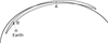 |
Fig. 1 Schematic illustration of the confidence curvilinear ellipsoid. Point A is the nominal position of the asteroid at time t, and point B is the VA on the main axis of the confidence ellipsoid at the same time, t, which is closest to the Earth after projection onto its TP. The arrow indicates the velocity direction of Earth with respect to the confidence ellipsoid. The bold line shows the nominal orbit of the asteroid. Image credit: Fig. 3 in (Vavilov 2020). |
2 Concept of the partial banana mapping method
Here we briefly outline the concept of the PBM method, which forms the core of our system. A more detailed discussion can be found in Vavilov & Medvedev (2015); Vavilov (2020).
The key assumption of PBM is that, over a considered time span, the uncertainties of the orbital elements evolve almost linearly from their values at the epoch of observations, t0. In other words, gravitational perturbations act in a similar way on the entire uncertainty region, so that most elements change coherently. In this case, the only orbital element that strongly differs is the mean anomaly – the angle that determines the position of the asteroid along its orbit. As a result, the uncertainty region is stretched primarily along the orbital path, while remaining narrow and close to the nominal trajectory. This elongated, curved region resembles the shape of a banana (see Fig. 1).
To describe this “banana-shaped” uncertainty region more accurately, we used a special coordinate system based on the osculating elliptical elements. In this system, one of the coordinates is the mean anomaly, M, and the other two (ξ, η) describe small shifts to the side and above or below the orbit (Vavilov & Medvedev 2015). This makes the uncertainty region easier to describe mathematically. In these curvilinear coordinates, the shape of the uncertainty region is often close to a six-dimensional Gaussian cloud.
The PBM method focuses on the part of the uncertainty region that might actually lead to an impact with the Earth. At the time of the possible impact, it searches along the largest axis of the uncertainty region for the point (point B in Fig. 1) that comes closest to the Earth, after projecting everything onto a TP (plane perpendicular to the asteroid-Earth relative motion). Once this closest point is found, PBM uses the local uncertainty shape around it to estimate the probability that the asteroid might hit the Earth. The method also finds the distance between point B and the Earth’s center in the TP, and the difference in M coordinates for the Earth and point A (nominal position of the asteroid).
3 NEOForCE monitoring system
Our impact monitoring system Near-Earth Object’s Forecast of Collisional Events uses a state vector (coordinates and velocities) and its 6 × 6 covariance matrix of an asteroid at the average time of observations. The covariance matrix, C0, gives us an approximation of the uncertainty of the state vector, x0, at time t0. If inside this uncertainty region there is a possible initial state vector that leads to a collision with the Earth, then the asteroid could potentially have an impact. The goal of a monitoring system is to find all significantly large areas of state vectors that lead to collisions, later referred as virtual impactors (VIs).
Our monitoring system consists of several stages. First, we cut the covariance matrix, C0, by many pieces and take VAs as representatives of these pieces (Sect. 3.1). Second, for each VA we compute all the times when the collision can happen around this VA (Sect. 3.3). Third, we combine the situations from the previous step, which indicate the same possible impact (Sect. 3.4). Fourth, we try finding a VI or claim that this possible collision is spurious (Sect. 3.5). Finally, we combine similar VIs (Sect. 3.6).
3.1 Initial sampling
In general the uncertainty region of an asteroid, especially a newly discovered one, even at the mean epoch of observations, is very elongated, in one preferred direction along an eigen vector. This preferred direction is also called the LOV (Milani et al. 2002). In the first stage, we sample VAs from the uncertainty region along the LOV. This line is determined as the eigen-vector of matrix C0 corresponding to the largest eigenvalue. Since matrix C0 is symmetric and positively defined, it can be decomposed by spectral decomposition:
 (1)
(1)
where U is an orthogonal matrix of the eigenvectors, Λ is a diagonal matrix of the eigenvalues, and T denotes the matrix transpose operation. The principal vector corresponding to the highest eigenvalue, λ11, determines the LOV.
We sample n VAs (in general n = 5001) on this line according to Laplace distribution so that the Laplace integral ( ) between two subsequent points is constant (and equalls the integral from the last point to infinity). We use
  to make the dispersion of the distribution equal one. Since we consider n VAs, the integral between the points equals b = 1/(n + 1). The VAs are then determined as follows:
 (2)
(2)
where li is the difference along the LOV from the nominal state vector.
We consider each VA to be a representative of its own vicinity. We assign the covariance matrix to each VA by exchanging the largest eigenvalue with  . Thus, a 1-sigma uncertainty ellipsoid around each VA would slightly touch or even include the neighbor VA. The covariance matrix determining the uncertainty region for a VA is computed with
 (3)
(3)
where Λ∗ is matrix Λ with  as the largest eigenvalue.
3.2 Initial check
Instead of running the NEOForCE system for all near-Earth asteroids, we first carry out the initial check as to whether this asteroid possibly can come close to the Earth. We select 100 VAs along the LOV (at 5σ intervals equidistantly), integrate their orbits into the future, and compute the minimal orbit intersection distance (MOID) between their orbits and the Earth’s orbit every 100 days. If the minimal MOID among all of them is greater than a certain threshold (0.02 au), we do not run the computation of the impact probability at all. Figure 2 presents this minimal MOID value for all of the asteroids that are in the impact risk table on the CNEOS website (on September 9, 2025), as well as the minimal MOID for all NEOs. As one can see, our threshold of 0.02 au includes all currently known NEAs with a nonzero impact probability. At the same time, it allows us to limit the number of launches of the monitoring system to approximately 15 000 instead of 40 000. This initial check requires less than one minute of computations for one asteroid on one thread of a processor such as Intel(R) Xeon(R) Gold 6230 2.10 GHz.
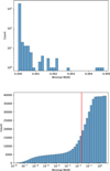 |
Fig. 2 Top: histogram of minimal MOID value for asteroids presented on the CNEOS website as the ones that have nonzero impact probabilities with the Earth on September 9, 2025. Bottom: cumulative histogram of minimal MOID for all NEOs. The vertical red line is our empirical 0.02 au threshold. |
3.3 Close encounter precomputation
In this step for each VA we compute the information about possible close encounters. We integrate the orbit of a VA with variational equations toward the future until the final time (in general, 100 years). In each integration step, we compute the osculating orbit of a VA and then obtain the minimal distance between the position of the Earth at this time and the points of this osculating ellipse (or parabola or hyperbola) numerically. We then find the local minima in these distances indicating the time of the local minima, t, the state vector of the VA,  , and the Earth, and the partial derivative matrix of VA’s state vector at t over the original time, t0: Φ(t0, t). The covariance matrix of the VA for time t is
 (4)
(4)
If the minimal distance between the osculating orbit and the Earth is <0.05 au, then we assume that a collision could not be ruled out at this time, t, for a vicinity of this VA.
We then use the concept of the PBM method (see Sect. 2). We construct the banana-shaped uncertainty region at time t for this VA using covariance matrix  , restricting it to 5σ uncertainty. In this region, we find the closest point to the Earth (point B in Fig. 1), its coordinates in the (ξ, η, M) coordinate system, and compute the distance between the Earth and the projection of point B to its TP. We also compute and save the difference in the mean anomaly, the M coordinate, between the found point, B, and point A.
We also estimate the maximal impact probability for this VA, assuming that its orbit leads to a collision with the Earth at time t, approximately. For this, we compute the full covariance matrix at time t around this VA:
 (5)
(5)
Then we hypothetically put the Earth at the center of the position of the VA at time t (point A in Fig. 1) and compute the probability by the TP method (Chodas 1993). To account for the distance from the VA to the nominal orbit, we then multiply this value by  , where li is from Eq. (2). This probability tells us the maximal possible value of the impact probability with the Earth that the selected asteroid can have at approximately time t around the vicinity of this VA. If it is lower than our threshold (nominally 5 × 10⁻⁸), we do not need to go to the next stage to find VIs. We consider this probability too low.
3.4 Selection of representatives
The information obtained in the previous step often indicates that several neighboring VAs along the LOV may correspond to the same potential encounter with the Earth. In particular, if a given close-approach time, t, is found, multiple VAs clustered around each other can all signal the possibility of a collision at that epoch. To avoid redundancy and to efficiently characterize each event, we identify a small set of representative VAs.
For each candidate epoch t, we first collect all VAs that point to a possible collision at approximately that time within 10 days. We then divide them by group so that each group consists of subsequent VAs along the LOV. Within each group, we search for two scenarios:
-
Earth located between two consecutive VAs (top panel in Fig. 3).
If the difference in the mean anomaly, M, computed in Sect. 3.4, shows opposite signs for two consecutive VAs, this implies that the Earth lies between them at the given time, t. In this case, we select the VA that is closest to the Earth at approximately time t. This VA becomes the selected representative. Note that this situation can happen several times within one group if the spread of VAs exceeds several revolutions around the Sun. The second VA we consider to be a “sidekick.”
-
Earth located on one side of the group (bottom panel in Fig. 3).
If the Earth is not bracketed by two VAs (i.e., all M differences have the same sign within the group), then we select only one VA – the one lying on the outer edge of the group and at the minimal distance to the Earth. This VA becomes the representative for the entire group.
Once we selected the representatives, we apply additional filters to them. First, as was mentioned above, we consider only the ones with a maximal impact probability of >5 × 10⁻⁸. Second, the distance between the Earth and the curved uncertainty region (distance between point B and the Earth) for at least one of the VAs must be smaller than 0.002 au. In the case in which the Earth is located between two subsequent VAs, even though we select only the closest one to the Earth, the representative is still selected if these two conditions are fulfilled for one of the VAs. If the conditions are not met, we do not expect that the collision could happen or that the probability is significant. And third, we only consider the ones for which the distance between the Earth and the VA at the time of the possible collision, t, is smaller than 1 astronomical unit. This limit with a 1 au distance allows us to exclude the situations in which the signs of M coordinate differences are opposite but the actual positions of the VAs are extremely far from the Earth (on the different side of the osculating orbit).
This filter allows us to consider only situations in which we believe the collision can happen, and only significant ones with sufficient impact probabilities. After this preselection, the next stage will find explicit orbital parameters around each selected VA that can lead to a collision, and estimate the impact probability.
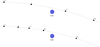 |
Fig. 3 Schematic illustration of the different scenarios for grouping of VAs. Top: Situation when the Earth is between two subsequent VAs (difference in M has opposite signs). In this case we chose j+1-th VA as our primary representative and j-th as a secondary one. Bottom: Situation when all the subsequent VAs are on one side from the Earth (difference in M are all positive). In this situation we chose j+2-th as our primary representative. Note that j+7-th VA is in another group but it will also be a representative of its group. |
3.5 Search for virtual impactors
Again, we follow the idea of Milani et al. (2005a) in the CLOMON2 system: that in order to confirm a possible collision one must explicitly find a VI (a state vector at initial epoch, t0, which actually leads to a collision). Therefore, in this stage we try to find the VI around each representative found in the previous step. For this we use a semi-linear approach extension of the PBM, briefly described here (for details see Vavilov & Hestroffer 2025).
The objective is to find the initial condition at epoch t0 of the asteroid, bringing it at time t to the closest point, B, in Fig. 1. The linear approximation reads as follows:
![Mathematical equation: ${\xi _ * } - \xi = \left[ {{{\partial \xi } \over {\partial {x_0}}}} \right]\left( {{x_{0 * }} - {x_0}} \right),$](/articles/aa/full_html/2026/03/aa57657-25/aa57657-25-eq14.png) (6)
(6)
where ξ and ξ∗ are vectors in the (ξ, η, M) coordinate system at time t of the asteroid (point A) and VA closest to the Earth on the main axis of curvilinear uncertainty ellipsoid (point B), correspondingly. x0 and x0∗ are the state vectors of the selected VA and the one that we are looking for, correspondingly, at t0 and ![Mathematical equation: $\left[ {{{\partial \xi } \over {\partial {x_0}}}} \right]$](/articles/aa/full_html/2026/03/aa57657-25/aa57657-25-eq15.png) is the matrix of the partial derivatives of curvilinear coordinates at time t over the Cartesian coordinates at t0.
is the matrix of the partial derivatives of curvilinear coordinates at time t over the Cartesian coordinates at t0.
 is the vector we are looking for to change the state vector of the selected VA on the previous stage so that after orbit integration it goes to point B at time t. In practice, for NEOForCE system we also use these two additional state vectors:
  and
and  . These state vectors are closer to x0 than
  . We integrate these orbits until time t plus 0.5 days. If none of them collide with the Earth at approximately time t, we select the one closest to the Earth. This newly selected VA is closer to the Earth at approximately time t than the original one, so we repeat the procedure using this VA as the new reference (starting from computing ξ, ξ∗ vectors and matrix
 ![Mathematical equation: $\left[ {{{\partial \xi } \over {\partial {x_0}}}} \right]$](/articles/aa/full_html/2026/03/aa57657-25/aa57657-25-eq20.png) ). In this way, the method works as an iterative refinement process: at each step the candidate VA is moved closer to the Earth at ≈ t until one of four conditions is met:
). In this way, the method works as an iterative refinement process: at each step the candidate VA is moved closer to the Earth at ≈ t until one of four conditions is met:
- (i)
a collision is found: we compute the probability with the TP method (see Sect. 4);
- (ii)
the solution drifts outside the 9σ uncertainty ellipsoid: we stop the procedure;
- (iii)
the maximum number of ten iterations is reached: we stop the procedure;
- (iv)
the asteroid enters the sphere of influence with the Earth – we run the TP analysis (see Sect. 4) to search for a VI.
By taking two additional state vectors that were closer to the original one instead of simply using  we slightly mitigate some convergence problems that can happen after multiple close encounters. In an extreme case in which the stretching of the uncertainty region is very high and mismatches the linear estimation, the closest VA between these three cases can be further away from the Earth than the original one. In this case we select
  VA and proceed again.
If a VI is found,  , we estimate its impact probability with the TP method and multiply this value by
![Mathematical equation: $\exp \left[ { - {1 \over 2}{{\left[ {{x_{0 * }} - {x_{\bf{0}}}} \right]}^{\rm{T}}}{\bf{C}}_0^{ - 1}\left[ {{x_{0 * }} - {x_{\bf{0}}}} \right]} \right],$](/articles/aa/full_html/2026/03/aa57657-25/aa57657-25-eq24.png) (7)
(7)
which takes into account that the found  is not the nominal one. If a VI is not found, we can use a “sidekick” to try to find a VI around it. We do not do it by default in order to save the performance but we keep this as an option for special cases.
3.6 Combination of similar impactors
In the last stage, we check if some of the found VIs are essentially the same and point to the same possible collision. For this we integrate the orbits of each VI until the impact, saving their positions every 30 days. If at each integration step several VIs are close to each other (distance <10−3 au), we take only the one with the highest impact probability value. We publish a possible collision if the impact probability is higher than 10−10. The reason why this threshold is significantly higher than the 5 × 10⁻⁸ threshold for the maximal impact probability is that if the maximal impact probability is too small it means the uncertainty of the asteroid around this area is too large. On the other hand, if the maximal impact probability is not too small but the actual impact probability of a VI is very low, this means that the uncertainty region only grazes the Earth rather than passing through its center. In such cases, even small changes in the nominal orbital solution can lead to large fluctuations in the estimated impact probability, which is why these cases are interesting.
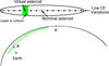 |
Fig. 4 Schematic illustration of the work of NEOForCE system. In the upper panel, one can see the nominal asteroid (purple dot), the original uncertainty region at the epoch of observation (black ellipse), the LOV (horizontal line), and VAs sampled along the LOV (black dots). The green area represents the smaller uncertainty region assigned to this VA. The red denotes the VI. In the bottom panel, one can see the nominal position of the asteroid at time slightly before a possible collision, t (point A), the osculating orbit of the nominal asteroid (black part of an ellipse), the Earth, the position of the VA (green dot), and the uncertainty region assigned for this VA at time slightly before t (curved green ellipse). The red dot (point B) represents the position of the VI. The dashed vector shows the relative motion of the Earth and the green uncertainty region. The Earth collides with the red dot. |
3.7 Short summary of the method
Below we provide a concise overview of the NEOForCE impact-monitoring algorithm. A schematic illustration of the work is shown in Fig. 4.
Sampling. We create many VAs along the LOV at the mean observation epoch (Sect. 3.1).
Initial screening. We conduct a first quick test to see whether the asteroid can ever come close to the Earth. For this, we compute the minimum MOID for a small group of VAs (Sect. 3.2).
Propagation and close-approach detection. We integrate the orbit of each VA into the future. We record every moment when the Earth come close to the osculating orbit of a VA (osculating ellipse), together with the time and distance (Sect. 3.3).
Curvilinear-region analysis. For every case in which the distance is smaller than 0.05 au, we build the curvilinear uncertainty region of the VA and compute its distance to the Earth. We also estimate the maximum impact probability that this VA can have (Sect. 3.3).
Selection of representative scenarios. From the previous step, we select only the most important situations: VAs that are neighbors along the LOV and that bracket the Earth at approximately the same time, have small distances between their uncertainty regions and the Earth, and show a noticeable impact probability (Sect. 3.4).
Search for VIs. For each selected case, we try to improve the VA’s state vector so that the VA hits the Earth. We do this step by step, coming closer to an impact solution. When the VA enters the Earth’s sphere of influence at the probable collision time, we use the target-plane analysis (Sects. 3.5 and 4).
Combine similar impactors. If two VIs stay very close to each other on their way toward the Earth, we treat them as the same solution and keep the one with the higher impact probability (Sect. 3.6).
4 Target plane analysis
4.1 Classical approach
The TP analysis begins with the integration of the asteroid’s orbit until its encounter with the Earth. Let ( ) be the state vector of the asteroid at the observational epoch, t0, derived from orbital fitting, and let C0 be its variance–covariance matrix. Integrating the orbit with variational equations (Battin 1964) up to the time, t, when the asteroid enters the Earth’s sphere of influence yields the state vector (
 ) and the partial derivative matrix
 (8)
(8)
The variance–covariance matrix at time t is then
 (9)
(9)
where T denotes the matrix transpose operation. Matrix  provides an approximation of the uncertainty region of an asteroid at time t.
The asteroid’s relative velocity with respect to the Earth, urel, is nearly the same for all VAs in this region, meaning that they share almost the same direction and speed. The TP is defined as the plane perpendicular to urel. The orientation of the coordinate axes on the plane is arbitrary; in our implementation we define them as
 (10)
(10)
where ξ, η, ζ are the axes of the new system, with ξ and ζ defining the coordinates on the TP, and z is the z axis in a Cartesian coordinate system. The center of the system is the asteroid.
To estimate impact probabilities, the 6D uncertainty region is projected onto the TP. An asteroid will collide with the Earth if the distance from the Earth’s center is smaller than its radius, R⊕ (see Fig. 5). Because of gravitational focusing, however, the asteroid’s trajectory inside the Earth’s sphere of influence is hyperbolic, so the effective cross section is larger. The minimum distance, q, is given by
 (11)
(11)
where vs ≈ 11.186 km s−1 is the Earth’s surface escape velocity, vinf is the unperturbed geocentric velocity, and b is the impact parameter (the distance on the TP between the projections of the Earth’s and asteroid’s centers).
Thus, a collision occurs when  . The effective collision radius is therefore
  .
.
The mapping from Cartesian state space (relative to the asteroid) to target-plane coordinates can be written as u = Bw, with a 2 × 6 matrix, B, and w being the relative to the nominal asteroid state vector. The covariance matrix on the TP is then  (Rao 1952). Placing the nominal solution at the origin, the impact probability reads
 (12)
(12)
where  is a circle with a radius of
  .
.
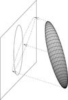 |
Fig. 5 Schematic illustration of the TP method. The ellipsoid represents the uncertainty region of an asteroid when it enters the sphere of influence, the plane is the TP, the circle on the plane is the projection of the Earth, and the ellipse on the plane is the projection of the ellipsoid. Image credit: (Vavilov 2018). |
4.2 Beyond the classical approach
The classical TP approach works well at typical encounter velocities. However, when the relative velocity is low, the encounter spans several days and the Earth’s motion can no longer be approximated as rectilinear. In such cases, the method can be inaccurate. This problem arises for asteroid 2000 SG344: for a possible impact on September 18, 2069, NEOForCE identified a VI, but the classical TP method estimated zero probability because the projected (ξ, ζ) coordinates of the Earth (reminder that in our system the asteroid is in the center) at entry into the Earth’s sphere of influence were too far from the center, despite an actual collision days later.
To address this, we adopt a modified approach similar to Milani et al. (2005a). We extend the integration until the epoch of closest approach and construct a “modified target plane (MTP)” perpendicular to the relative velocity at that instant. If the asteroid collides with the Earth, the MTP is defined at the impact point. Using the relative position and velocity at closest approach, we compute the unperturbed velocity, v∞, and derive the corresponding unperturbed target-plane coordinates ( ) from the MTP coordinates (ξMTP, ζMTP):
 (13)
(13)
where E is the total orbital energy, µ = GM⊕/R⊕, and M⊕, R⊕ are the Earth’s mass and radius, respectively. For high-speed encounters,  , but at low velocities the difference is significant.
Since the covariance matrix gives an adequate estimation of the uncertainty region only before the entry into the sphere of influence, we approximate the mapping between TP1 (classical TP at entry) and TP2 (unperturbed TP built from MTP) as a rotation by an angle, α, and a scale factor, sc, estimated from
 (14)
(14)
For 2000 SG344, sc can exceed 1.3, while α is only a couple of degrees. The relative velocity, u∞, is also significantly different from urel, and hence the corrected gravitational focusing radius of the Earth,  changes. That is why we sometimes had a situation in which we found a VI but the (ξTP, ζTP) coordinates were further away than the corrected radius of the Earth, which of course led to wrong impact probability values. We therefore map
  onto TP1, rotate by α, and scale by sc to obtain the 2 × 2 matrix
  .
.
4.3 Search for virtual impactor
To confirm whether a potential encounter corresponds to a genuine collision, we follow the method of Milani et al. (2005a). The 6D state vector at t relative to the nominal state vector of the asteroid can be partitioned into [r, s], where r = (ξTP, ζTP) are target-plane coordinates and s is the complementary 4D vector.
We seek the adjusted state, ![Mathematical equation: $[\hat r,\hat s]$](/articles/aa/full_html/2026/03/aa57657-25/aa57657-25-eq46.png) , corresponding to a collisional orbit with the highest probability density. The procedure is to: 1. Compute
, corresponding to a collisional orbit with the highest probability density. The procedure is to: 1. Compute  from Eq. (13). 2. Obtain
  by rotating and scaling CTP. 3. Select
  inside
  that minimizes
  . 4. Transform back to TP1 to get
  .
.
The covariance matrix, C, of [r, s] at time t can be decomposed as
 (15)
(15)
According to (Milani et al. 2005a) , the vector s∗ can be found from
 (16)
(16)
We then search for the vector  at the epoch of observations, t0, that leads to the vector [r∗, s∗] at time t, and hence to the collision. The linear relation reads
![Mathematical equation: $\left[ {\left( {{r_ * },{s_ * }} \right)} \right] - [(r,s)] = {\bf{W}} \cdot {\bf{\Phi }}\left( {{t_0},t} \right)\quad \left( {{{\tilde x}_{0 * }} - {x_{0 * }}} \right),$](/articles/aa/full_html/2026/03/aa57657-25/aa57657-25-eq56.png) (17)
(17)
where W is the 6 × 6 rotation matrix into the TP2 frame. As in Sect. 3.5 we also consider  and
and  and select the closest one to the Earth at time t. If all these three are more distant than
  at time t, we take
  .
.
If the state vector,  , does not lead to a collision approximately at time t, this process needs to be iterated taking
  as
as  and using Eqs. (16) and (17). If the procedure does not determine a collision after ten iterations or is outside of the 9σ 6D ellipsoid, we consider this impactor to be spurious.
Comparison table for asteroid 2008 EX5.
5 Practical realization and discussion
In this version of the system, we used collocational integrator Lobbie of the 14th order (Avdyushev 2022) to integrate the orbits. In the model we included the gravitational influence of eight major planets (and the dwarf planet Pluto, for historical reasons), as well as post-Newtonian formalism for the Sun only. We also considered the Earth and the Moon separately. The orbits of the asteroids and their covariance matrices were taken from the DynAstVO database4 Desmars et al. (2017) for the automated impact monitoring.
Comparison table for asteroid 2005 QK76.
5.1 Completeness problem
The completeness of our system is determined by the threshold of impact probability that can be detected certainly. Following (Milani et al. 2005a) one can estimate the generic completion level: the highest impact probability that can be missed by our monitoring system if the uncertainty trail on the TP is fully linear.
Under these assumptions, a possible collision can be missed if both representatives found in Sect. 3.4 are further than 1 au from the Earth. This literally means that the distance between two subsequent VAs at the time of this possible collision exceeds 2 au along the orbit. According to the sampling of VAs along the LOV, the maximal integral probability of a Gaussian distribution on the interval between two subsequent VAs is approximately 3 × 10⁻⁴. This is slightly higher than if we sampled VAs along the LOV according to a Gaussian distribution. In this case, the probability would be 2 × 10⁻⁴. Our objective is hence the following: if we took a sample of 5001 VAs according to the Gaussian distribution, the latest VAs would be only 3.54 sigmas away from the nominal state vector (l2500 = 3.54 from Eq. (2)). By sampling the Laplace distribution l2500 = 5.53 instead, we have VAs much further from the nominal state vector, without losing much in terms of completeness. Hence, the highest impact probability that can be missed is approximately
![Mathematical equation: ${{{D_ \oplus }[au]} \over {2{\rm{au}}}}3 \times {10^{ - 4}}.$](/articles/aa/full_html/2026/03/aa57657-25/aa57657-25-eq66.png) (18)
(18)
To take into account the gravitational focusing of the Earth in order to properly estimate the completeness, we need to increase the diameter of the Earth, D⊕, by  (Chodas 1993), where ve is the escape velocity from the Earth’s surface (≈ 11.186 km/s) and v∞ is the unperturbed geocentric velocity (approximately the velocity when crossing the sphere of influence). When the relative velocity of an asteroid and the Earth is high, the diameter of the Earth does not change much and is about 10−4, which makes the completeness be around 1.5 × 10⁻⁸. However, for a very slow-moving asteroid (with 1 km/s relative velocity) the diameter is 11.22 times larger, which lowers the completeness to 1.7 × 10⁻⁷. In Sect. 3.4 we exclude all the representatives with an estimated maximal impact probability lower than 5 × 10⁻⁸, which sounds reasonable.
Comparison table for asteroid 2023 DO.
Comparison table for asteroid 2000 SG344 (beginning).
Computation times and the number of VI searches for five considered asteroids.
5.2 Comparison to Sentry
To evaluate the robustness of our system, we performed detailed comparisons using five representative asteroids: 2005 QK76, 2008 JL3, 2023 DO, 2008 EX5, and 2000 SG344. We selected these asteroids from the web-page Sentry of Central for Near-Earth Objects Study (CNEOS)5. We were looking for objects at the top of the list with a high cumulative impact probability and a significant number of possible impacts with probabilities higher than 5 × 10⁻⁷ in order to be able to make a comparison. The asteroids have different observational arcs (from 1.7 days to 1.4 years) and different numbers of observations (from 14 to 52). In each case, we adopted the same orbital solutions and the same covariance matrices as those used by NASA’s Sentry-II system, retrieved via the NASA SSD API6 on September 9, 2025, so that the results would be directly comparable.
The outcomes of our system and Sentry-II are presented in the tables below. In each table, “Date” refers to the epoch of the possible collision identified by NEOForCE, while PNEOForCE and PNASA are the corresponding impact probabilities computed by our system and Sentry-II, respectively. We attempted to match VIs such that, for collisions occurring at similar epochs, both the probability and the distance metric σVI are comparable.
σVI quantifies how far a VI lies from the nominal orbit in terms of standard deviations and is defined as
![Mathematical equation: $\sigma _{VI}^2 = {\left[ {{x_{0 * }} - {x_0}} \right]^{\rm{T}}}{\bf{C}}_0^{ - 1}\left[ {{x_{0 * }} - {x_0}} \right],$](/articles/aa/full_html/2026/03/aa57657-25/aa57657-25-eq70.png) (19)
(19)
where  is the state vector of the VI, x0 is the nominal state vector, and C0 is the covariance matrix.
It is important to note that similar σVI values do not necessarily imply that the same VI was found: many VAs can lie on the same 5D ellipsoidal surface defined by a given σVI. Conversely, two very similar VIs may have different σVI values; for example, a small shift in the direction of the smallest eigenvector of C0 can leave the overall trajectory nearly unchanged while significantly altering σVI.
Comparison table for asteroid 2008 JL3.
5.2.1 Asteroid 2008 EX5
Asteroid 2008 EX5 is newly discovered, with 61 observations spanned over 32 days. Its cumulative impact probability is about 4.5 × 10⁻⁵, not very high, and it also has only a few significant possible impacts. Table 1 shows an agreement between two systems, with Sentry losing eight possible collisions with probabilities of less than 1 × 10⁻⁷ (below the mentioned completeness level) and NEOForCE losing seven possible collisions with probabilities of less than 5 × 10⁻⁸, below the threshold for maximal impact probability.
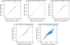 |
Fig. 6 Comparison between the NEOForCE impact monitoring system and Sentry-II. This figure summarizes the results from Tables 1–5. We show only impact probabilities larger than 10−9. A point located on the horizontal line at PNASA = 10−9 indicates a potential impact identified by NEOForCE but not detected by Sentry-II. Conversely, a point on the vertical line indicates an impact detected by Sentry-II but not found by NEOForCE. |
5.2.2 Asteroid 2005 QK76
Asteroid 2005 QK76 was discovered on August 30, 2025. There are only 14 observations of it, spanning 1.67 days. Such a short observation arc makes its orbit highly uncertain and a good test for comparison. As one can see from Table 2, there is no significant difference in the impact probabilities of the possible collisions found. However, the values of σVI are substantially different, with larger values for Sentry-II. Sentry-II did not find the possible collision on February 26, 2038, with an impact probability of 1.7 × 10⁻⁷, but this is at the completeness limit of Sentry-II.
5.2.3 Asteroid 2023 DO
This asteroid was observed over a relatively long arc of 41 days, with 52 recorded observations. Discovered on February 13, 2023, it has 25 possible collisions published by Sentry-II. As is shown in Table 3, our NEOForCE system identified 47 possible collisions in total. Of these, NEOForCE did not reproduce five solutions listed by Sentry-II, all with impact probabilities below 6.7 × 10⁻⁸, close to our completeness threshold of 5 × 10⁻⁸. Conversely, Sentry-II missed 27 possible collisions detected by NEOForCE, including one with a probability of 1.79 × 10⁻⁶ on March 23, 2085, another at 5.1 × 10⁻⁷ on March 23, 2060, and one at 8.4 × 10⁻⁸ on March 24, 2061.
5.2.4 Asteroid 2008 JL3
This asteroid was observed over a short arc of only 7 days, yielding 35 measurements in total. Discovered on May 2, 2008, it has 44 possible collision solutions listed in Sentry-II. A comparison of our system with Sentry-II (Table 6) shows that NEOForCE identified 87 possible collisions but did not recover three mentioned by Sentry-II, all with impact probabilities below 4.6 × 10⁻⁹ – way below our completeness threshold. In contrast, Sentry-II missed 46 possible collisions, including one with the highest reported impact probability of 1.26 × 10⁻⁶ on April 28, 2109, as well as three others with probabilities exceeding 10−7.
5.2.5 Asteroid 2000 SG344
Asteroid 2000 SG344 turns out to be a hard test for our systems. It was discovered on September 29, 2000, by the LINEAR survey at Socorro, New Mexico. The orbital solution used today by NASA JPL is based on observations spanning from May 15, 1999, to October 3, 2000, giving it an observational arc of about 1.4 years, with only a modest number of measurements available for orbit fitting (31 observations). Its orbital period is nearly one year, the inclination relative to the ecliptic is almost zero, and the aphelion lies just beyond Earth’s orbit. These parameters result in very low encounter velocities with Earth (about 1.4 km/s) and a continuum of predicted close approaches after several resonance returns after 2070. Because of this unusual dynamical configuration, 2000 SG344 has been the subject of a dedicated impact-hazard study (Chodas & Chesley 2001).
Sentry-II system indicates 300 possible impacts of this asteroids with the Earth, of which 138 have probabilities higher than 10−6. NEOForCE system found 1363 possible impacts and 172 with probabilities >10−6.
For the reasons discussed above, the computation time for asteroid 2000 SG344 was significantly higher (more then six times longer than for 2008 JL3). Table 5 reports the total computation time, obtained in parallel mode using two threads on an Intel(R) Xeon(R) Gold 6230 CPU at 2.10 GHz, together with the number of situations in which the VI search procedure was triggered.
A summary of the comparison for all five considered asteroids with NASA is shown in Fig. 6. For asteroids 2008 EX5, 2005 QK76, 2023 DO, and 2008 JL3, we find a good agreement between the two systems, with impact probability values consistent down to the 10−7 level, except for a few missing collision cases. For asteroid 2000 SG344, the agreement is noticeably worse and holds only down to about the 10−6 level. In this case, several potential collisions at the 10−5 probability level are missed by the NASA system. This behavior is likely caused by the very small relative velocity during close encounters, which reduces the completeness of the monitoring system (see Sect. 5.1).
6 Conclusions
In this work, we present NEOForCE (Near-Earth Object’s Forecast of Collisional Events), a newly developed and fully independent monitoring system for predicting potential asteroid impacts with the Earth. The system is designed to operate autonomously from existing services and will ultimately use orbital solutions provided by the Paris Observatory. A central feature of NEOForCE is its search strategy: rather than testing encounters with the VAs themselves, it identifies epochs when the Earth approaches the curvilinear uncertainty regions of the propagated VAs. This approach, combined with an assessment of the encounter’s maximal impact probability, allows the system to efficiently narrow down possible collisions, and proceed to a targeted search for VIs only when warranted. In the search for VIs, we use the semi-linear PBM method, which can successfully find an impactor even if the VA is at a 1 au distance from the Earth.
We validated NEOForCE by comparing its performance with NASA’s Sentry-II system on five asteroids with different orbital and observational characteristics. The results demonstrate that NEOForCE reliably reproduces almost all of the significant impact solutions reported by Sentry-II above the 10−7 probability level, confirming the robustness of the method. Moreover, NEOForCE identified additional low-probability impact solutions (in the 10−7–10−6 range) that Sentry-II did not report. These tests show that NEOForCE provides a reliable and complementary tool for impact monitoring, strengthening the independence and robustness of global planetary defense capabilities.
Data availability
The full version of Table 4 is available at https://doi.org/10.5281/zenodo.18344255.
Acknowledgements
This project has received funding from the European Union’s Horizon 2020 research and innovation programme under the Marie Sklodowska-Curie grant agreement #101068341 “NEOForCE”.
References
- Avdyushev, V. A. 2022, Sol. Syst.Res., 56, 32 [Google Scholar]
- Battin, R. H. 1964, Astronautical Guidance, eds. R. Bracewell, C. Cherry, W. W. Harman, E. W. Herold, J. G. Linvill, S. Ramo, & J. G. Truxal (New York, San Francisco, Toronto, London: McGraw-Hill Book Company), 338 [Google Scholar]
- Chodas, P. W. 1993, BAAS, 25, 1236 [Google Scholar]
- Chodas, P. W., & Chesley, S. R. 2001, in AAS/Division of Dynamical Astronomy Meeting, 32, 08.03 [Google Scholar]
- Desmars, J., Thuillot, W., Hestroffer, D., David, P., & Le Sidaner, P. 2017, in European Planetary Science Congress, EPSC2017-324 [Google Scholar]
- Milani, A. 1999, Icarus, 137, 269 [Google Scholar]
- Milani, A., Chesley, S. R., Boattini, A., & Valsecchi, G. B. 2000, Icarus, 145, 12 [NASA ADS] [CrossRef] [Google Scholar]
- Milani, A., Chesley, S. R., Chodas, P. W., & Valsecchi, G. B. 2002, Asteroid Close Approaches: Analysis and Potential Impact Detection, 55 [Google Scholar]
- Milani, A., Chesley, S. R., Sansaturio, M. E., Tommei, G., & Valsecchi, G. B. 2005a, Icarus, 173, 362 [Google Scholar]
- Milani, A., Sansaturio, M. E., Tommei, G., Arratia, O., & Chesley, S. R. 2005b, A&A, 431, 729 [NASA ADS] [CrossRef] [EDP Sciences] [Google Scholar]
- Rao, C. R. 1952, Advanced Statistical Methods in Biometric Research (New York: John Wiley & Sons), 53 [Google Scholar]
- Roa, J., Farnocchia, D., & Chesley, S. R. 2021, AJ, 162, 277 [NASA ADS] [CrossRef] [Google Scholar]
- Vavilov, D. E. 2018, Trans. IAA RAS, 14 [in Russian] [Google Scholar]
- Vavilov, D. E. 2020, MNRAS, 492, 4546 [NASA ADS] [CrossRef] [Google Scholar]
- Vavilov, D. E., & Hestroffer, D. 2025, A&A, 699, A158 [NASA ADS] [CrossRef] [EDP Sciences] [Google Scholar]
- Vavilov, D. E., & Medvedev, Y. D. 2015, MNRAS, 446, 705 [NASA ADS] [CrossRef] [Google Scholar]
All Tables
All Figures
|
Fig. 1 Schematic illustration of the confidence curvilinear ellipsoid. Point A is the nominal position of the asteroid at time t, and point B is the VA on the main axis of the confidence ellipsoid at the same time, t, which is closest to the Earth after projection onto its TP. The arrow indicates the velocity direction of Earth with respect to the confidence ellipsoid. The bold line shows the nominal orbit of the asteroid. Image credit: Fig. 3 in (Vavilov 2020). |
| In the text | |
|
Fig. 2 Top: histogram of minimal MOID value for asteroids presented on the CNEOS website as the ones that have nonzero impact probabilities with the Earth on September 9, 2025. Bottom: cumulative histogram of minimal MOID for all NEOs. The vertical red line is our empirical 0.02 au threshold. |
| In the text | |
|
Fig. 3 Schematic illustration of the different scenarios for grouping of VAs. Top: Situation when the Earth is between two subsequent VAs (difference in M has opposite signs). In this case we chose j+1-th VA as our primary representative and j-th as a secondary one. Bottom: Situation when all the subsequent VAs are on one side from the Earth (difference in M are all positive). In this situation we chose j+2-th as our primary representative. Note that j+7-th VA is in another group but it will also be a representative of its group. |
| In the text | |
|
Fig. 4 Schematic illustration of the work of NEOForCE system. In the upper panel, one can see the nominal asteroid (purple dot), the original uncertainty region at the epoch of observation (black ellipse), the LOV (horizontal line), and VAs sampled along the LOV (black dots). The green area represents the smaller uncertainty region assigned to this VA. The red denotes the VI. In the bottom panel, one can see the nominal position of the asteroid at time slightly before a possible collision, t (point A), the osculating orbit of the nominal asteroid (black part of an ellipse), the Earth, the position of the VA (green dot), and the uncertainty region assigned for this VA at time slightly before t (curved green ellipse). The red dot (point B) represents the position of the VI. The dashed vector shows the relative motion of the Earth and the green uncertainty region. The Earth collides with the red dot. |
| In the text | |
|
Fig. 5 Schematic illustration of the TP method. The ellipsoid represents the uncertainty region of an asteroid when it enters the sphere of influence, the plane is the TP, the circle on the plane is the projection of the Earth, and the ellipse on the plane is the projection of the ellipsoid. Image credit: (Vavilov 2018). |
| In the text | |
|
Fig. 6 Comparison between the NEOForCE impact monitoring system and Sentry-II. This figure summarizes the results from Tables 1–5. We show only impact probabilities larger than 10−9. A point located on the horizontal line at PNASA = 10−9 indicates a potential impact identified by NEOForCE but not detected by Sentry-II. Conversely, a point on the vertical line indicates an impact detected by Sentry-II but not found by NEOForCE. |
| In the text | |
Current usage metrics show cumulative count of Article Views (full-text article views including HTML views, PDF and ePub downloads, according to the available data) and Abstracts Views on Vision4Press platform.
Data correspond to usage on the plateform after 2015. The current usage metrics is available 48-96 hours after online publication and is updated daily on week days.
Initial download of the metrics may take a while.