| Issue |
A&A
Volume 707, March 2026
|
|
|---|---|---|
| Article Number | A257 | |
| Number of page(s) | 18 | |
| Section | Astrophysical processes | |
| DOI | https://doi.org/10.1051/0004-6361/202557739 | |
| Published online | 10 March 2026 | |
Born to be recycled: A comprehensive population synthesis of the Galactic millisecond pulsars
1
Université de Strasbourg, CNRS, Observatoire astronomique de Strasbourg, UMR 7550, 67000 Strasbourg, France
2
National Centre for Radio Astrophysics, Tata Institute for Fundamental Research, Post Bag 3 Ganeshkhind, Pune 411007, India
3
Université de Strasbourg, Télécom Physique Strasbourg, F-67400 Illkirch-Graffenstaden, France
4
Janusz Gil Institute of Astronomy, University of Zielona Góra, ul. Szafrana 2, 65-516 Zielona Góra, Poland
★ Corresponding author: This email address is being protected from spambots. You need JavaScript enabled to view it.
Received:
17
October
2025
Accepted:
28
January
2026
Abstract
Context. Millisecond pulsars (MSPs) are the oldest and fastest pulsars known to date. The first MSP to be discovered was PSR B1937+21 in 1982. To explain how these pulsars could be formed, a new hypothesis was formulated: the recycling of pulsars, i.e the fact that a pulsar could accrete matter from a companion and be spun up.
Aims. In this study we develop a population synthesis algorithm for pulsars that belong to a binary in order to check whether most of the observed recycled pulsars were formed via an accretion mechanism, and we derive statistics about their properties that are difficult to obtain through observations. We also make predictions for future surveys.
Methods. Towards the presented objectives, we used the code Stellar EVolution for N-body (SEVN) in order to take all the binary processes into account and our own code to evolve each pulsar self-consistently by considering the secular evolution of a force-free magnetosphere, the magnetic field decay, gravitational braking, and spatial evolution. Each pulsar was born in a binary with a main sequence companion and evolved to the present time. The radio and γ-ray emission locations were modelled using the polar cap geometry and striped wind model, respectively.
Results. Our simulations reproduce well the population of radio and γ-ray pulsars observed in the selected surveys, as supported by Kolmogorov-Smirnov (KS) tests. We also found that there should be fewer than 220 unidentified recycled pulsars in the Fourth Fermi-LAT catalogue of γ-ray sources. Most of the pulsars accrete for typical durations of 108 − 9 yr. Moreover the typical timescale of alignment between the rotation axis and the normal to the orbital plane (angle α) usually remains much shorter. As a consequence, ∼80% of the binary pulsar population has α close to 0°. Most of the recycled pulsars possess masses around 1.8 M⊙, and some have masses up to 2.7 M⊙, in agreement with recent observations of spider pulsars, which are massive. We estimate that ∼190 MSPs originally born in the Galactic spiral arms contribute to ∼5% of the γ-ray galactic center excess, reinforcing the fact that if this excess is entirely of pulsar origin, these MSPs must have come from globular clusters that migrated inwards to the Galactic centre or were born in the bulge. High values of the viewing angle, ζ, seem to be needed to be able to observe the recycled pulsars, and it also seems difficult to observe recycled pulsars with an aligned rotation axis and magnetic axis (i.e. χ ≤ 10°). We find that only a small fraction, approximately ∼7.6 × 10⁻³%, of oxygen-neon white dwarfs in binary systems appear to contribute to the population of mildly recycled pulsars through accretion-induced collapse.
Key words: gravitation / methods: statistical / binaries: general / pulsars: general / gamma rays: stars / radio continuum: stars
© The Authors 2026
 Open Access article, published by EDP Sciences, under the terms of the Creative Commons Attribution License (https://creativecommons.org/licenses/by/4.0), which permits unrestricted use, distribution, and reproduction in any medium, provided the original work is properly cited.
This article is published in open access under the Subscribe to Open model. This email address is being protected from spambots. You need JavaScript enabled to view it. to support open access publication.
1. Introduction
Millisecond pulsars (MSPs) represent the oldest objects in the entire population of pulsars. Although they are at the very end of stellar evolution, they are the fastest spinning pulsars known (with periods P < 30 ms). In contrast to normal isolated pulsars and magnetars, MSPs are found in binary systems, a fact that provides strong evidence of the rapid rotation. During the binary evolution stage, they likely accreted matter from their companion, which increased their angular momentum and spun them up to high rotational frequencies (Alpar et al. 1982; Bhattacharya & van den Heuvel 1991; Tauris et al. 2012). More broadly, these objects are referred to as ‘recycled pulsars’, as they are thought to have initially undergone a significant spin-down before being spun up again. During the accretion phase, these sources have been observed as X-rays binaries (Wijnands & van der Klis 1998; Patruno & Watts 2021). Although different mechanisms (accretion process, magnetic field decay) are involved in recycling of pulsars, they are not completely understood. Nevertheless the recycling scenario is widely accepted in the community today (Radhakrishnan & Srinivasan 1982; Yang & Li 2023; Tauris & van den Heuvel 2023). MSPs without a companion have also been observed, and their properties compared to recycled pulsars with a companion are not distinguishable, which supports the idea that all recycled pulsars must have been related to binary evolution at some point (Srinivasan & van den Heuvel 1982). Moreover, recycled pulsars appear in various forms. Some are isolated, as mentioned earlier (Backer et al. 1982); others have a companion that can be degenerate or not; and in some cases the MSP in the binary can be considered a spider. These include black widows, where the pulsar’s very light companion (M < 0.05 M⊙) is being destroyed by the pulsar wind, and redbacks, which have more massive companions (M ∼ 0.1 − 0.4 M⊙) that are ablated by the pulsar (Roberts 2013; Blanchard et al. 2025). Furthermore, transitional MSPs are sources that switch between X-ray and radio emitters (Papitto & de Martino 2022). In eclipsing MSPs, the radio emission is eclipsed by the companion and could be due to ejected ionised material from the companion that is absorbing the radio waves from the MSP (Fruchter et al. 1988). Finally, MSPs with planets also exist (Wolszczan & Frail 1992).
Until 2008, very few pulsars had been detected in γ-rays (about seven; Thompson 2008), and it is thanks to the Fermi Gamma-Ray Space Telescope (Fermi) that this number was significantly increased to about 300 today (Smith et al. 2023). Only a few MSPs have been detected in gamma-rays without a radio counterpart. Already in the 1990s, it was proposed that many MSPs might be γ-ray sources (Srinivasan 1990), and Fermi has since led to a dramatic increase in the number of detected γ-ray MSPs, although the vast majority of known MSPs have been discovered through radio observations. Radio pulsar surveys, such as those conducted with the Parkes, Arecibo, and Green Bank telescopes; the Five-hundred-meter Aperture Spherical Telescope (FAST); and MeerKAT, have identified over 400 MSPs to date (Manchester et al. 2005; Qian et al. 2020; Bailes et al. 2020), many of which were later found to emit in γ-rays as well. Radio observations remain essential for accurately determining pulsar timing parameters, detecting binary companions, and characterising their orbital dynamics. Furthermore, several MSPs are still only visible in the radio domain, highlighting the complementarity of multiwavelength studies.
A powerful tool for investigating neutron star (NS) evolution is population synthesis. Numerous studies have applied this method to different NS families, including the normal pulsar population (Faucher-Giguère & Kaspi 2006; Gullón et al. 2014; Sautron et al. 2024; Pardo-Araujo et al. 2025), magnetars (Jawor & Tauris 2022; Beniamini et al. 2019; Sautron et al. 2025), and MSPs (Kiel et al. 2008; Story et al. 2007; Gonthier et al. 2018; Tabassum & Lorimer 2025). From the simulations in these studies, invaluable insights can be extracted regarding the underlying population properties such as the birth spin period, magnetic field decay timescale, and birth rate as well as the emission processes at play. In this approach, NSs are generated at birth and evolved to the present epoch, after which detection criteria are applied to determine whether they would be observable with current or future instruments.
In this work, we focus exclusively on mildly or fully recycled pulsars (a mildly recycled pulsar has accreted matter but not enough to become fully recycled with P < 30 ms, and thus it has 30 ≤ P ≤ 1000 ms and a Ṗ < 10−16) that are not in globular clusters (GCs). Although about half of the known population of MSPs belong to a GC, studying pulsars that are in GCs is very different. Indeed, to study them accurately with simulations, we would need to take many interactions into account. Since there are high stellar densities in these environments (much higher than the Galactic field), we would need to take into account the fact that there could be an exchange of companions (at least it should happen more compared to the Galactic field), there could be triple systems, or there might be a different distribution at birth for the eccentricity or the semi-major axis of the binary. For instance, Berteaud et al. (2024) used simulation-based inference (Cranmer et al. 2020) to study the MSP population in GCs, and they focused on Terzan 5 by finding constraints on the luminosity function of its MSPs and the number (with uncertainties) of MSPs that Terzan 5 hosts.
Story et al. (2007) and Gonthier et al. (2018) are the most complete studies about the population synthesis of MSPs. The less recent study of Story et al. (2007) made predictions for Fermi and revealed that many MSPs would be detected by it as radio quiet γ-ray sources, which was indeed true (Abdo et al. 2013; Smith et al. 2019, 2023). In their paper, the evolution of the MSPs started after their spun-up episode was finished, the magnetic field of MSPs was constant, and only MSPs from the Galactic disc were considered. The more recent study of Gonthier et al. (2018) improved on the studied sample by considering MSPs in the bulge, too. They predicted that 11 000 MSPs would be necessary in the Galactic bulge to explain the γ-ray galactic center excess detected in the Galactic centre, and their results are in agreement with those derived from Fermi detections. Although the results of Gonthier et al. (2018) are compelling, our approach, which self-consistently models the full binary evolution alongside the pulsar’s evolution and a detection model in the γ-ray and radio to reproduce the recycled population, offers several advantages. Our study is so far the only one that allows to follow the full evolution to the MSP state and even to produce mildly recycled pulsars while taking into account the detectability in both radio and γ-ray wavelengths. Our study constitutes a valuable opportunity to investigate whether the accretion-driven formation channel is an effective pathway for producing MSPs, especially in comparison to alternative scenarios such as the collapse of white dwarfs (WDs) into rapidly rotating NSs. Moreover, it enables the derivation of statistical properties of the recycled population, which can be otherwise difficult to access observationally. Finally, it allowed us to make predictions for upcoming surveys, such as the Square Kilometre Array (SKA1).
This paper explores many aspects of the binary evolution leading to recycled pulsars. It is organised as follows. In Sect. 2 we describe the model to generate and evolve the pulsars. We describe the model to detect the pulsars in the simulation in Sect. 3. Finally, the results are presented in Sect. 4, discussed in Sect. 5, and summarised in Sect. 6.
2. Evolution model
Compared to previous studies, the novelty of the present work lies in the careful treatment of the evolution of binary systems up to the formation of compact objects in their final stage. At the beginning of the simulation, all of the secondary stars considered in the binaries are main sequence (MS) stars that are at a certain percentage of their lives. This percentage is taken from a random uniform distribution between 0 and 100%, while the NS in the binary starts at age 0. We begin by presenting the stellar evolution code, Stellar EVolution for N-body (SEVN), followed by a description of the binary processes it includes. We then introduce the adopted birth distributions and initial characteristics, and outline the prescriptions implemented for the evolution of NSs. Next, we discuss the spatial evolution of the systems, before finally addressing the concept of the death valley.
2.1. The SEVN code
The SEVN code is a state-of-the-art binary population synthesis code. It models single stellar evolution by interpolating pre-computed stellar tracks on the fly, and accounts for binary interactions using analytic and semi-analytic prescriptions (Spera & Mapelli 2017; Spera et al. 2019; Mapelli et al. 2020; Sgalletta et al. 2023). In this work, we used the version of SEVN described in Iorio et al. (2023)2. In Sects. 2.2, 2.3, 2.4, and 2.5 we detail a general overview of the main features that we used from SEVN, with modifications on the NS evolution proposed by SEVN to get the best description possible. We refer to Iorio et al. (2023) for a detailed description of the code. The SEVN code requires a maximum NS mass that can be reached in the simulation to be set. Thus, we selected this maximum to be 3 M⊙, as in the work of Sgalletta et al. (2023).
2.2. Binary processes
Various binary processes come into play during the course of binary evolution, in the following we describe the ones relevant in this work that are implemented in SEVN. The Roche lobe RL, of a star in a binary system defines the region of space within which matter remains gravitationally bound to the star. When a star fills its Roche lobe, material can flow towards the companion star under the influence of its gravitational pull, a process known as Roche-lobe overflow (RLO). The RLO affects several key parameters, including the mass ratio, the individual masses and radii of the stars, and the binary’s semi-major axis. At each time step, SEVN evaluates the Roche-lobe radii of both stars using the analytical formula derived by Eggleton (1983):
 (1)
(1)
If the radius of the companion of the NS satisfies r ≥ RL, then an RLO episode starts and mass falls from the secondary star, which filled its Roche lobe, to the NS (the opposite case is also possible, although very unlikely as the system would need to be very compact). The mass transfer can then either be stable or unstable. In order to decide in which case the system is, in SEVN when the mass ratio q is greater than a critical value qc that depends on the stellar evolutionary phase, the mass transfer is unstable on a dynamical timescale. The values of qc used are the same as in Hurley et al. (2002), Spera et al. (2019), Giacobbo & Mapelli (2020); see the values in the first column of Table 3 in Iorio et al. (2023).
A stable mass transfer results in the mass-loss rate, Ṁd, proposed by Hurley et al. (2002):
 (2)
(2)
where F(Md) is a normalisation factor, Rd is the radius of the donor and RL, d is the Roche lobe of the donor star. SEVN accounts for non-conservative mass transfer, meaning that the donor star can lose more mass than the companion actually accretes. The accreted mass, Ṁa, is then modelled according to the following prescription:
 (3)
(3)
where ṀEdd is the Eddington accretion rate and fMT is the mass accretion efficiency, which is within the range [0,1]. In SEVN, fMT = 0.5 (Bouffanais et al. 2021; Iorio et al. 2023).
In the case of unstable mass transfer, the binary results in either a merger or a common envelope (CE). There are debates in the community about if it is possible to have spin-up during the CE phase (Osłowski et al. 2011; MacLeod & Ramirez-Ruiz 2015; Chamandy et al. 2018; Chattopadhyay et al. 2020). Because of the controversy, spin-up during CE is not included in SEVN. Therefore, if the mass transfer is not stable, in this simulation the pulsar cannot be recycled, and that is why we do not describe the CE evolution here (but see Iorio et al. 2023; Sgalletta et al. 2023 for more details).
2.3. Birth properties
Many birth characteristics generated for each pulsar are independent of their companion, such as the position in the Galaxy (x0,y0,z0), inclination angle (χ0), spin period (P0), magnetic field (B0). Therefore, these quantities are generated from the same distributions, with the same parameters, as described in the paper of Sautron et al. (2024). However, compared to our study of the normal pulsars, we did change two elements in this work: firstly, the kick velocity distribution was modified by adopting a lower dispersion of σv = 70 km s−1 which better matches the recycled pulsar population and is consistent with earlier works (Story et al. 2007; Gonthier et al. 2018). Indeed, this prescription is to reflect the assumption that the binary survived the supernova explosion of the primary star that formed the NS. All simulated systems are thus assumed to remain bound after the first supernova event that initially formed the NS in the binary. Furthermore, this prescription provides a better match to the recycled pulsar population, as a high velocity dispersion would result in the loss of a large fraction of systems (resulting in ∼3.5 times fewer detectable NSs), thereby requiring a significantly higher birth rate to reproduce the observed population. Nevertheless, if the secondary star undergoes a supernova explosion to become an NS or a black hole (BH) later in the evolution, the binary may still be disrupted due to the associated mass loss and natal kick from the formed NS or BH, as implemented in the SEVN code. Secondly, instead of using the radial distribution in the galactic plane of Yusifov & Küçük (2004), we used a truncated normal distribution (the distribution is truncated to be always greater than 0) with a mean μR = 11.3 kpc, and a standard deviation σR = 1.8 kpc to have the NSs born in the spiral arms (see Sautron et al. 2024 to check how the NSs are then placed into the spiral arms). Actually, using the radial distribution proposed by Yusifov & Küçük (2004) causes too many pulsars in the Galactic centre to be detected compared to observations. That is why we opted for the truncated normal distribution for the radial distribution in the spiral arms, which was also an option in Faucher-Giguère & Kaspi (2006) and Tabassum & Lorimer (2025).
The population of NS generated have their ages taken from a random uniform distribution between a minimum age of 5 × 10⁷ yr, as it is very unlikely that a pulsar can be recycled within a shorter time, and a maximum age of 13.9 × 10⁹ yr, which is within the range of the estimated age of the universe (Riess et al. 1998). In each simulation, the number of sources is characterised by a birth spacing X, where X is chosen as an integer number of years between the births of subsequent pulsars. In this paper, we report this quantity as either the birth spacing X in years or the birth rate Rrecycled = (1/X) yr−1. This approach can be used to verify whether a constant birth rate is realistic, by comparing the results from the simulation to observation. Before running the simulation, we choose the number of binaries, and then by computing  at the end of the simulation, we get the birth rate. In this work, simulating between 4.6 × 10⁵ and 5.7 × 10⁵ pulsars in a binary allowed us to get similar P−Ṗ diagram between observations and simulations, resulting in a birth rate between 3.3 − 4.1 × 10⁻⁶ yr−1. We discuss the birth rate range obtained in Sect. 5.
The mass of the NS progenitor (M1) is drawn from Kroupa’s initial mass function (Kroupa 2001), within the range [8–25] M⊙ (Belczynski & Taam 2008):
 (4)
(4)
Although our simulation starts with the NS already formed, meaning we are ultimately interested in its initial mass, we still need to know the progenitor mass in order to determine the mass of the companion star. This is because the mass ratio of the binary,  (with M2 being the mass of the secondary star), is drawn from a power-law distribution as suggested by Sana et al. (2012):
 (5)
(5)
Then, we computed M2 by deriving q and M1. Each pulsar has its birth mass, MNS, i, drawn from a Gaussian distribution such as
 (6)
(6)
where μM = 1.33 M⊙ and σM = 0.09 M⊙. This distribution is derived from a fit of the Galactic binary NS masses (Özel et al. 2012; Özel & Freire 2016). Our independent sampling of progenitor mass and NS mass removes the statistical correlation whereby more massive progenitors tend, on average, to produce more massive NSs (Sukhbold et al. 2016). This may influence the NS mass distribution obtained in this work. MSPs are very fast rotating NSs. Therefore, for P < 6.5 ms, we can no longer neglect the spin-down caused by gravitational waves (GWs); see Appendix A for more details. We can define a triaxial inertia tensor that is diagonalised on the basis of its principal axes. These axes are denoted by e1, e2, e3 with the corresponding moments of inertia given by I1 = I, I2 = I(1 + ϵ12) and I3 = I(1 + ϵ13) respectively. The terms ϵ12 and ϵ13 characterise the ellipticity, i.e. the degree of deviation from perfect stellar sphericity. However, in our case we assumed we only had biaxial stars, which is sufficient for our purposes, as considering triaxial stars would significantly increase the complexity without providing additional physical insight beyond the key requirement that the stars are deformed. Therefore, we have ϵ12 = 0 and ϵ13 = ϵ ≠ 0. Thus, for each NS, we drew its ellipticity ϵ from a log uniform distribution between [–13,–5] in order to have a value of ϵ between [10−13, 10−5]. These limits are suggested by the study of Giliberti & Cambiotti (2022).
The SEVN code also requires the metallicity of the secondary star. As it would necessitate taking into account the environment and the past of the binaries to have an accurate value taken for the metallicity, no assumption was made about it. The metallicity, Z, was taken from a random log-uniform distribution between [0.0002,0.02]. Furthermore, still concerning the secondary star, SEVN also needs the initial ratio Ωs/Ωc, which is the spin frequency of the star over its critical spin frequency, we take it from a uniform distribution between [0,1]. We chose a uniform distribution over all possible values of this ratio, as we found that the choice of distribution had little influence on the results.
The binary eccentricity (e) distribution was derived from a power law, as suggested by the study of Sana et al. (2012), where they found this distribution for massive binaries:
 (7)
(7)
The semi-major axis (a) of the binary was drawn from a distribution that is flat in log(a) for wide binaries and decreases smoothly at close separations, as proposed by Han et al. (2020):
 (8)
(8)
where ψsep ≈ 0.070, a0 = 10 R⊙, a1 = 5.75 × 10⁶ R⊙, R⊙ ≈ 696 340 km and m ≈ 1.2. We do not claim that these distributions represent the exact initial distributions for NS+MS binaries, which are currently unknown. Nevertheless, they cover the relevant parameter space for a and e, and using uniform distributions over the same ranges does not reproduce the observed population as well. Therefore, we retained the distributions of a and e for massive binaries, even though they may not accurately reflect reality. The angle between the rotation axis of the NS and the normal to the orbital plane, which we call α, the spin-orbit angle is assumed to follow an isotropic distribution generated from a uniform distribution U ∈ [0, 1] and given by α = arccos(2 U − 1).
2.4. Neutron star evolution
2.4.1. General evolution model
Because SEVN evolves pulsars in a vacuum as they spin down, we changed the evolution proposed by SEVN with a force-free model evolution taking into account the plasma in the magnetosphere. Further, we adapted the model from Biryukov & Abolmasov (2021) to also take into account the GW emission if the NS reaches a spin frequency Ω ≥ 960 rad.s−1. As soon as the NS reaches Ω < 960 rad.s−1 again, the GWs are neglected. While a fully accurate treatment would require modelling the impact of GWs on the inclination and spin-orbit angle evolution, we neglect these effects as they would greatly complicate the model, while most of the time the GW emission can still be neglected. Thus, in this work the evolution of an NS can be described by the following set of differential equations:
 (9a)
(9a)
 (9b)
(9b)
 (9c)
(9c)
where  is the moment of inertia of the NS (we assume the spherical formula for I, although we consider an ellipticity ϵ for the NS, as this ϵ is very small, between 10−13 and 10−5). The torques n1, n2, n3, nGW are respectively, the averaged torques acting on the NS caused by accretion, magnetic braking due to magnetic field-disc interaction, pulsar’s radiation loss and gravitational braking due to a non-null ellipticity. The coefficient η is set to unity as suggested by Biryukov & Abolmasov (2021). It describes the accretion torque modulation within the spin period. The term A(η, α, χ) is a normalisation function:
![Mathematical equation: $$ \begin{aligned} A\left(\eta ,\alpha ,\chi \right) = \left[1- \frac{\eta }{2}\left(\sin ^2\chi \sin ^2\alpha +2\cos ^2\chi \cos ^2\alpha \right)\right]^{-1}. \end{aligned} $$](/articles/aa/full_html/2026/03/aa57739-25/aa57739-25-eq15.gif) (10)
(10)
The torques are defined by
 (11a)
(11a)
 (11b)
(11b)
 (11c)
(11c)
 (11d)
(11d)
Here, G is the gravitational constant, MNS is the mass of the NS, ṀNS is the mass accretion rate of the NS,  is the magnetic moment with the permeability constant μ0 = 4π × 10−7 H/m, R = 12 km is the radius of the NS, and c = 3 × 10⁸ m/s is the speed of light in vacuum. The different radii defined, i.e. rin, rco and rlc, are respectively the inner disc radius, the co-rotation radius, and the light cylinder radius:
 (12a)
(12a)
 (12b)
(12b)
 (12c)
(12c)
where ξ ∼ 0.5 is a dimensionless factor accounting for the detailed disc structure (Bessolaz et al. 2008).
It is not straightforward to visualise the temporal evolution of a pulsar in the P−Ṗ diagram from this system of differential equations. Therefore, we provide in Sect. 2.7 an example of the typical evolutionary track of a pulsar that becomes a recycled pulsar.
2.4.2. Spin-down
When the NS is not accreting matter, n1 and n2 are set to zero, and the star spins down as a result. Additionally, nGW is also set to zero when Ω < 960 rad.s−1. When these conditions are satisfied, we can apply the simplified set of equations from Sautron et al. (2024), which consider only the pulsar’s radiative losses. This approach allows for faster computation compared to solving the full system of Eqs. (9a), (9b), and (9c). The equations are given by
 (13a)
(13a)
![Mathematical equation: $$ \begin{aligned} \ln (\sin \chi _0) + \frac{1}{2\sin ^2\chi _0} +&K \Omega _0^2 \frac{\cos ^4\chi _0}{\sin ^2\chi _0} \frac{\alpha _d \tau _d B_0^2}{\alpha _d - 2} \left[\left(1+\frac{t}{\tau _d}\right)^{1-2/\alpha _d}-1\right] \nonumber \\ = \ln (\sin \chi ) + \frac{1}{2\sin ^2\chi }, \end{aligned} $$](/articles/aa/full_html/2026/03/aa57739-25/aa57739-25-eq25.gif) (13b)
(13b)
where the quantities with a subscript of 0 indicate their value at birth. Those without a subscript display their current value at present time. The time t represents the true age of the pulsar and K = 4πR6/Iμ0c3. Equation (13a) is the integral of motion between Ω and χ, the inclination angle, and Eq. (13b) allowed us to find the evolution of χ in a dipolar configuration with a magnetic field decay. This system was found by Philippov et al. (2014) for a spherically symmetric NS with a constant magnetic field and Dirson et al. (2022) adapted Eq. (13b) for a decaying prescription. Finally, when there is no accretion and Ω ≥ 960 rad.s−1, we solve still Eqs. (9a) and (9c), with n1 = n2 = 0.
2.4.3. Spin-up
As mentioned earlier, the NS can spin-up only if it is accreting matter, as n1 is the only torque that is positive. Therefore, only n1 can increase Ω. Two conditions are necessary for the NS to accrete matter. First, the companion must reach its Roche lobe, and then the NS needs to have its Keplerian angular velocity at the inner disc radius (ΩK|rin) be greater than its co-rotation angular velocity (Ωco):
 (14)
(14)
Thus, Ωdiff > 0 is necessary for the NS to be accreting matter, the inner disc radius rin is defined by Eq. (12a). When matter reaches the inner disc radius, the magnetic pressure dominates, forcing the material to follow the magnetic field lines and funnel onto the NS’s polar caps. However, if Ωdiff < 0, the NS enters the propeller regime: the magnetic field lines at the magnetic radius rotate faster than the local Keplerian velocity, preventing accretion and expelling the matter away from the star (Abolmasov et al. 2024).
2.4.4. Magnetic field evolution
The evolution of NS magnetic fields remains a subject of debate. Some early pulsar population synthesis studies suggested that the magnetic field does not evolve over time (Bhattacharya et al. 1992; Faucher-Giguère & Kaspi 2006). However, several physical mechanisms support the idea of magnetic field decay, including ohmic dissipation in the crust, ambipolar diffusion in the core, crustal vortex motion, internal turbulence, and energy loss through radiation (Srinivasan et al. 1990; Cumming et al. 2004; Dall’Osso et al. 2012; Viganò et al. 2013). A recent study that includes ohmic heating (Igoshev & Popov 2024), along with period derivative measurements and spectral data from the NS RX J0720.4-3125, further suggests a rapid decay of its magnetic field. Moreover, more recent population synthesis studies have shown that models incorporating magnetic field decay provide a great match to the observed pulsar population (Gullón et al. 2014; Sautron et al. 2024). Therefore, we adopted a magnetic field decay following a power-law prescription:
 (15)
(15)
where αd is a constant parameter controlling the speed of the magnetic field decay, B0 the initial magnetic field, Bmin the minimum magnetic field reachable by the NS, t corresponds to the elapsed time since the birth of the NS and τd the typical decay timescale. We use αd = 1.5 (as in Sautron et al. 2024 for the normal pulsars). Concerning τd, we considered three different values randomly chosen for the generated pulsar, 0.05, 1.4, and 2.3 Myr, with a probability of 0.77, 0.115, and 0.115 to have these values, respectively. These three probabilities effectively approximate the probability density function of τd and were sufficient to reproduce the recycled pulsar population. Determining the full distribution of τd would require further investigation beyond the scope of this study. Physically, the τd distributions represent the range of possible evolutionary trajectories in the P–Ṗ diagram for recycled pulsars, similar to Fig. 10 in Viganò et al. (2013). Thus, each pulsar in the simulation follows one of three possible evolutionary paths, an empirical approach that reproduces the P–Ṗ distribution better than using a single path. These discrete values were selected purely by trial and error. Whether the NS is accreting or not, the magnetic field is decaying in this model; however accretion-induced field decay was also taken into account.
As the NS accretes matter from its companion, this matter goes along the magnetic field lines to the polar caps. Progressively, the matter accreted can apply enough pressure to compress and bury the magnetic field under the NS surface (Payne & Melatos 2007; Wang et al. 2012). This accretion-induced field decay process can be described by
 (16)
(16)
where B(t) is computed via Eq. (15) to model the decay caused by the other physical mechanisms mentioned earlier, ΔMNS is the amount of accreted mass by the NS and ΔMd is the magnetic field decay mass scale. Typically the accreted mass by an NS is less than 0.5 M⊙ (Özel & Freire 2016; You et al. 2025) and we adopt ΔMd = 0.025 M⊙ as in the work of Chattopadhyay et al. (2020) which is the optimal value found in their study.
To prevent the magnetic field of NSs from dropping to unrealistically low values, we imposed for each pulsar a minimum magnetic field value, Bmin, randomly drawn from a uniform distribution in the range [103, 104] T. This range is motivated by the study of Zhang & Kojima (2006), who investigated the lower limits that NS magnetic fields can realistically attain.
2.5. Spatial evolution
The motion of each binary’s centre of mass within the Galactic potential is evolved in the gravitational potential Φ. They are subject to an acceleration  given by
 (17)
(17)
We integrate numerically Eq. (17) with a position extended Forest Ruth-like (PEFRL) algorithm (Omelyan et al. 2002), a fourth order integration scheme. Concerning the galactic potential, the Galaxy is divided in four distinct regions, which results in four different potentials: the bulge Φb and the disc Φd which have the form proposed by Miyamoto & Nagai (1975), the dark matter halo Φh which has the form proposed by Navarro et al. (1997) and the nucleus Φn represented by a Keplerian potential. The total potential of the Milky Way Φtot is the sum of these potentials:
 (18)
(18)
See Sautron et al. (2024) for a detailed analysis of the PEFRL scheme, its accuracy, and for the detailed expression of the galactic potentials used.
Although SEVN does not integrate the full orbital motion of binaries with respect to their centre of mass, it computes the evolution of the semi-major axis and eccentricity using prescriptions for mass exchange within the system, following Eqs. (15) and (16) of Hurley et al. (2002). The dominant processes affecting these orbital parameters are tides, which are modelled through Eqs. (34)–(36) of Iorio et al. (2023, see Sects. 2.3.1 and 2.3.4 of their paper for more details about wind mass transfer and tides respectively). In addition, SEVN accounts for the evolution of the semi-major axis and eccentricity driven by GW emission. Peters (1964) describes in his work the orbital decay and circularisation caused by GWs with the following equations:
 (19a)
(19a)
 (19b)
(19b)
where G is the gravitational constant, m1 and m2 are the masses of the two stars in the binary, c is the speed of light, a is the semi-major axis and e is the eccentricity of the orbit. In SEVN, these equations are solved when the GW merger timescale, tmerge becomes shorter than the Hubble time. See Appendix D of Iorio et al. (2023) for more details about the computation of the GW merger timescale.
2.6. Death valley
Spread in the parameter values of the model causes significant variations in the death line, and thus a death valley rather than a single death line describes the condition for pulsar extinction in the P−Ṗ diagram. Nonetheless, this death valley must be based on a death line definition, we choose to extend the death line from Mitra et al. (2020), originally defined for normal pulsars to access the criteria for generation of coherent radio emission given as follows:
 (20)
(20)
Here, T6 = T/106 K, where T corresponds to the surface temperature of the polar cap and P is the spin period of the pulsar in s. The parameter η = 1 − ρi/ρGJ is the electric potential screening factor due to the ion flow, where ρi corresponds to the ion charge density and ρGJ to the Goldreich-Julian charge density above the polar cap. The quantity b is the ratio of the actual surface magnetic field to the dipolar surface magnetic field and χl is the angle between the local magnetic field and the rotation axis. In order to obtain the death valley in Fig. 1, the parameters described above are drawn from distributions, found and described in Sautron et al. (2024).
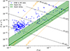 |
Fig. 1. Diagram of P−Ṗ of the observed pulsars considered in this work along with the death line (solid green line) and the death valley (shaded green area). |
2.7. Evolution in the P−Ṗ diagram of a recycled pulsar
To better visualise how a pulsar evolves in the P−Ṗ diagram to become a recycled pulsar, Fig. 2 shows the track followed by a pulsar evolving in the simulation, starting with an initial period P0 = 9.7 × 10⁻² s, period derivative Ṗ0 = 2.7 × 10⁻¹³ s/s, and mass MNS, 0 = 1.38 M⊙, its companion being a ∼8 M⊙ main sequence star. Since the mass ratio of these two stars,  , exceeds the critical mass ratio for main sequence stars in the simulation, qc = 3.0, it means that the mass transfer would be unstable. This implies that a CE phase must have occurred, allowing the secondary star to lose enough mass in the envelope, which was then ejected, for the system to later enter a stable mass-transfer phase. For further details on binary evolution, see Tauris & van den Heuvel (2023). We can basically distinguish three major phases in the evolution of this pulsar: first, the pulsar was dominated by the spin-down (caused mostly by the torque n3 presented in 2.4) and evolved towards a spin period close to 10 s. Then, when the accretion started (after 0.21 Gyr of evolution) we can clearly see that the pulsar, which passed the death line before, comes back from the commonly called graveyard of pulsars to have a very rapid rotation, close to the millisecond, thanks to the spin-up (caused by the torque n1 presented in 2.4) that dominates this phase. Finally, when the accretion ends (the accretion lasted ∼0.33 Gyr), the pulsar can continue to evolve by being dominated once again by spin-down. However, compared to when the pulsar was young, the spin-down is much weaker, due to the reduced value of the magnetic field, which is now much lower than at its birth, that is why ∼10 Gyr after the end of the accretion phase, the pulsar barely moved in the P−Ṗ diagram. The pulsar finished its evolution with P = 1.9 × 10⁻³ s, Ṗ = 1.1 × 10⁻²⁰ s/s, MNS = 2.3 M⊙ (thus, the pulsar accreted ∼0.9 M⊙) and ended up isolated as its companion was ejected after its supernova explosion.
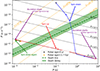 |
Fig. 2. Evolution in the P−Ṗ diagram of a pulsar in the simulation that becomes an MSP. |
3. Detection model
In this section we address the detectability of our simulated pulsars in both radio and γ-ray wavelengths. First of all, in this work we exclusively consider two radio surveys, the FAST Galactic Plane Pulsar Snapshot (GPPS) survey (Han et al. 2021) and the Parkes Multibeam Pulsar Survey (PMPS; Manchester et al. 2001), as these surveys detected the most MSPs. For the γ-ray wavelengths, we are interested in the comparison of the results of our simulation with the detections obtained by the Fermi/LAT instrument. Therefore, we compared the γ-ray pulsars obtained in our simulation with the pulsars from the Third Fermi Large Area Telescope Catalog (3PC).
For each pulsar, we verified whether it met the detection criteria based on three factors. The first is the beaming fraction, which represents the portion of the sky swept by the radiation beam and depends on the wavelength (radio or γ-ray), the spin rate, geometry, and emission region. Before detailing how the radio and γ-ray beaming fractions are computed, we first define the relevant angles.
The angle between the line of sight and the rotation axis is  , where nΩ = Ω/||Ω|| is the unit vector along the rotation axis, and n is the unit vector along the line of sight. The inclination angle between the rotation axis and the magnetic moment is
  , with μ the unit vector along the magnetic moment. Finally, the impact angle
  is related by χ + β = ζ.
We chose an isotropic distribution for the Earth viewing angle, ζ, as well as for the orientation of the unitary rotation vector. The Cartesian coordinates of the unit rotation vector, nΩ, are (sin θnΩ cos ϕnΩ, sin θnΩ sin ϕnΩ, cos θnΩ). We set the Sun’s position at (x⊙, y⊙, z⊙) = (0 kpc, 8.5 kpc, 15 pc) (Siegert 2019). The coordinates for n are
 (21)
(21)
To compute the pulsar distance from Earth, we used the formula for the distance,
 (22)
(22)
3.1. Radio detection model
The beaming fraction in radio depends on the half opening angle of the radio emission cone, ρ. Since our selected sample of observed pulsars includes a few pulsars with P > 0.1 s, the half opening angle, ρ, of simulated pulsars that reach a similar value is computed according to Lorimer & Kramer (2004) by
 (23)
(23)
where hem is the emission height, P is the pulsar spin period, and c is the speed of light. The emission height was assumed to be constant with an average value of hem = 3 × 10⁵ m, based on observational estimates from a sample of pulsars (Weltevrede & Johnston 2008; Mitra 2017; Johnston & Karastergiou 2019; Johnston et al. 2023). The cone half-opening angle, ρ, as defined in Eq. (23), applies only to the last open field lines of a dipolar magnetic field and is valid primarily for slow pulsars, where the emission altitude is high enough for higher-order multi-polar components to be negligible. For fast pulsars, however, relativistic effects due to rapid rotation become significant and must be taken into account (Xilouris et al. 1998). Furthermore, little is known about the characteristics of the half-opening angle and the emission height in fast pulsars. For this reason, and since we adopted a purely dipolar geometry for all pulsars, even though multi-polar components are expected to play a role in reality, we retained a formula similar to Eq. (23) following the prescription of Kijak & Gil (1998, 2003) for ρ:
 (24a)
(24a)
 (24b)
(24b)
where ralt denotes the emission altitude in units of NS radii, and μalt and σalt are respectively the mean and standard deviation of the Gaussian distribution (f(ralt)) from which ralt is drawn. Running multiple simulations showed that adopting μalt = 8 RNS and σalt = 4 RNS provides the best agreement with observations, meaning that both radio pulse profiles and the fraction of γ-ray pulsars that could be visible in radio are consistent with the observations.
A pulsar can be detected in radio if β = |ζ − χ|≤ρ or β = |ζ − (π − χ)| ≤ ρ, corresponding to visibility from the northern or southern magnetic hemisphere, respectively. An additional useful quantity is the radio pulse width, wr, which is computed following Lorimer & Kramer (2004) as
 (25)
(25)
For radio flux density, we use a formula similar to that in Johnston et al. (2020), designed for 1.4 GHz observations by the Parkes telescope in the southern Galactic plane (Kramer et al. 2003; Lorimer et al. 2006; Cameron et al. 2020) and Arecibo in the northern plane (Cordes et al. 2006). The main difference in this work lies in the power-law dependence on the spin-down luminosity  . Johnston & Karastergiou (2017) found that using Ė0.5 overpredicted young pulsars, while Ė0 overrepresented old ones; they adopted Ė0.25 as a compromise. In our case, we found that lowering the exponent to 0.125 improved agreement with observations. Thus, the flux density formula is
 (26)
(26)
where d is the distance in kpc and Fj is the scatter term which is modelled as a Gaussian with a mean of 0.0 and a variance of σ = 0.2. The detection threshold in radio is set by the signal-to-noise ratio defined by
 (27)
(27)
We directly compute the radio flux, without computing the luminosity in radio that overlooks the fact that the luminosity received will depend on the geometry of the beam. A pulsar is detected in radio if its signal-to-noise ratio exceeds the threshold imposed by FAST GPPS Han et al. (2021) or PMPS Manchester et al. (2001). Indeed, in this work we focus exclusively on these two radio surveys. The region of observations of these surveys are taken into account; see Table 1. S/N depends on  which is the minimum detectable flux, which is related to the instrumental sensitivity, the period of rotation P and the observed pulse profile width of radio emission
  . To compute the observed pulse profile width, we adopted the same formula as in Cordes & McLaughlin (2003):
 (28a)
(28a)
![Mathematical equation: $$ \begin{aligned} S_{\mathrm{survey}}^{\mathrm{min}}&= \frac{C_{\rm thres} [T_{\rm sys}+ T_{\rm sky}(l,b)]}{G \sqrt{N_p \ B \ t }} \sqrt{\frac{\tilde{w}_r}{P-\tilde{w}_r}}\cdot \end{aligned} $$](/articles/aa/full_html/2026/03/aa57739-25/aa57739-25-eq51.gif) (28b)
(28b)
Survey parameters of PMPS and the FAST GPPS.
Equation (28a) accounts for interstellar medium (ISM) density fluctuations, including dispersion (τDM) and scattering (τscat) caused by interactions with free electrons in the Galaxy during the radio pulse’s propagation. Instrumental effects are also considered through the sampling time, τsamp. More details on these parameters are provided in Appendix B.
In Eq. (28b), where we detail the expression of the minimum detectable flux, Cthres is the detection threshold of the survey, Tsys is the system temperature in K, G is the telescope gain in K.Jy−1, Np is the number of polarisations, B is the total bandwidth in Hz and t is the integration time in s. The quantities which have just been presented, are the survey characteristics, which depend on whether we consider FAST GPPS or PMPS (see Table 1). Tsky is the sky background temperature in K, at the longitude l and latitude b. Remazeilles et al. (2015) provided a refined version of the temperature map of Haslam et al. (1982). Since the data were obtained at 408 MHz, in order to rescale to the correct observing frequencies, a power-law dependence is assumed with the form Tsky ∝ f−2.6 (Johnston et al. 1992). We use Eq. (28b) to compute the minimum flux required for radio detection.
3.2. γ-ray detection model
The γ-ray emission model is based on the striped wind scenario, where γ-ray photons are produced in the current sheet of the pulsar wind. Detection requires the observer’s line of sight to lie near the equatorial plane, with the inclination angle satisfying |ζ − π/2|≤χ. The γ-ray luminosity is taken from the study by Kalapotharakos et al. (2019), who found it follows a fundamental plane relation. Their full 3D model depends on the magnetic field B, the spin-down luminosity Ė, and the cut-off energy ϵcut. Since our PPS does not include ϵcut, we adopted the simplified 2D version of their model:
 (29)
(29)
Here, Ė is the spin-down luminosity, and the associated γ-ray flux detected on Earth is computed with
 (30)
(30)
where fΩ is a factor depending on the emission model reflecting the anisotropy. For the striped wind model, Pétri (2011) showed that this factor varies between 0.22 and 1.90. In this work, we use an updated version of Fig. 7 of Pétri (2011), and it allowed us to obtain fΩ when the viewing angle, ζ, and the inclination angle, χ, are known. Therefore, this update allowed us to get more realistic values for fΩ between 0.13 and 316. See Appendix C for more details on using the force-free model. The pulsar is detected in gamma depending on the instrumental sensitivity as described below.
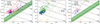 |
Fig. 3. Diagram of P−Ṗ for observed and simulated pulsars in different wavelengths. Left panel: P−Ṗ diagram for the detected pulsars in radio surveys only in the simulations in red along with the observations in radio for the FAST GPPS or PMPS survey in blue. Middle panel: P−Ṗ diagram for the detected pulsars in γ-ray surveys only in the simulations in green, along with the observed pulsars in γ-ray from Fermi surveys only in blue. Right panel: P−Ṗ diagram for the simulated pulsars detected both in radio and γ-ray surveys in purple, along with observations for the FAST GPPS or PMPS survey simultaneously with the γ-ray observations from Fermi in blue. For all the panels, the death line is represented as a green solid line, and the death valley is the shaded green area. |
The γ-ray sensitivity is determined based on the expected performance of the Fermi/LAT instrument3. For each simulated pulsar, we consult the all-sky sensitivity map provided by Fermi/LAT4. At the position defined by the Galactic longitude (l) and latitude (b) of the pulsar, we retrieve Fmin, the minimum detectable flux at that location. If Fermi/LAT did not observe the region, this is also taken into account. A pulsar is considered detectable in γ-rays if its γ-ray flux (Fγ) exceeds the local threshold (Fmin).
4. Results
4.1. Radio versus γ-ray pulsars
The first goal of this study was to match the P−Ṗ diagram between simulation and observations in order to assess whether the recycling process could primarily explain the observed pulsar population of mildly and fully recycled pulsars in the P−Ṗ diagram (i.e. pulsars with B ≤ 5 × 10⁶ T). By using the parameters for the various distributions at birth and the evolution model presented in Sect. 2, we obtained the three P−Ṗ diagram in Fig. 3. The left panel displays the diagram for pulsars detected only in radio surveys, the middle panel for those detected only in γ-rays surveys, and the right panel for pulsars detected in both radio and γ-rays surveys. In each case, observations are shown alongside simulations. For the radio-only population (left panel), the Kolmogorov–Smirnov (KS) test (Smirnov 1948) yields a p-value of 5.6 × 10⁻⁵ for the spin period P distribution and 0.2 for the spin-down rate Ṗ distribution. This suggests that the null hypothesis is rejected for P but not for Ṗ. Nevertheless, the simulated population matches observations well for P < 0.1 s, with p-values greater than 0.05 for both P and Ṗ, indicating that few recycled pulsars are observed above this value, meaning this channel of formation only allows one to obtain a few mildly recycled pulsars, but not all of them. In the ATNF catalog, 167 radio pulsars detected by the FAST GPPS or PMPS surveys have measured values of both P and Ṗ. Additional detections exist but are sometimes missing a Ṗ measurement – such detections were excluded from the comparison with our simulation. Other additional detections may also exist that are not yet included in the catalog. A more complete list of sources can be found online5. In our simulation, we detect 176 radio pulsars, which agrees reasonably well with the number of radio pulsars discovered by FAST GPPS and PMPS. Furthermore, the death valley eliminates ∼100 pulsars, and most of them were well below the valley. Regarding, the middle panel (pulsars in γ-ray surveys only), most of the observed pulsars appear to be reproduced in the simulation, though there is a noticeable over-detection for Ṗ > 3 × 10⁻²⁰. From 3PC, 137 pulsars were selected for comparison (still with the criterion: B ≤ 5 × 10⁶ T), of which 20 were also detected by the selected radio surveys, leaving 117 as pulsars in γ-ray surveys only. In the simulation, 98 such pulsars were detected with Ṗ < 3 × 10⁻²⁰. When comparing this observed sample to the simulated one (restricted to Ṗ < 3 × 10⁻²⁰), the KS test yields p-values of 0.15 for Ṗ and 0.25 for P, indicating good agreement. Furthermore, the number of detected pulsars in both datasets is very similar. The overabundance of simulated pulsars with Ṗ > 3 × 10⁻²⁰ could correspond to unidentified sources in the Fourth Fermi-LAT catalogue of γ-ray sources (4FGL), or may reflect limitations of the striped wind model. These interpretations are further discussed in Sect. 5. Finally, the population of pulsars detected in both radio and γ-ray surveys (right panel) is too small for a robust KS test. However, the simulated pulsars occupy a similar region of the P–Ṗ space as the observed ones. The simulation does show an excess of approximately 20 pulsars compared to observations, which corresponds well to the number of radio MSPs associated with γ-ray sources that have not yet been observed to pulsate in the 4FGL catalogue (Abdollahi et al. 2022). These observed sources may simply not have shown detectable pulsations so far, and further investigations could reveal their MSP nature, which would be consistent with our simulation results.
Although the middle panel displays what we classified as pulsars in γ-ray surveys only, we still computed their expected radio flux using Eq. (26). This choice is motivated by the fact that, once a pulsar is detected in γ rays, it is often followed up with dedicated radio observations. As a result, most of the γ-ray pulsars eventually have some form of radio measurement associated with them. However, these follow-up observations are not linked to any specific survey. As a result, in the ATNF data, many γ-ray pulsars that do emit in radio are not listed as being associated with a radio survey, which is the criterion we used to classify pulsars as either radio-loud or radio-quiet in Fig. 3. Consequently, ∼71% of the objects we label as pulsars in γ-ray surveys only in the simulation actually have radio fluxes greater than 30 μJy and a geometry that would allow one to see pulsations, i.e |ζ − χ|≤ρ, which in real observations would almost always lead to a radio detection (Smith et al. 2023). Indeed, in the sample of 117 pulsars used in this work from the 3PC catalogue labelled as pulsars in γ-ray surveys only, only 6 of them actually lack any radio detection, either from surveys or from targeted observations. This corresponds to 94.9% of γ-ray pulsars not seen in a radio survey, which have a radio counterpart.
We compare the simulated and observed γ-ray light-curve peak separation, Δ, in Fig. 4. The separation, Δ, was computed according to Pétri (2011) with
 (31)
(31)
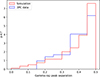 |
Fig. 4. Distribution of the γ-ray peak separation of the simulated population along with the observations from the 3PC catalogue. |
Here, ζ is the angle between the line of sight and the rotation axis, and χ is the magnetic inclination angle. All distributions are normalised to yield probability distribution functions (PDFs) by dividing each PDF by the total number of pulsars–observed or simulated. Since the signal is periodic and the definition of the main peak is arbitrary, the peak separation (Δ) is restricted to the interval [0, 0.5]; values larger than 0.5 are mapped to 1 − Δ via a phase shift. Figure 4 shows a striking agreement between the observed and simulated γ-ray peak separation distributions, indicating that the striped wind model reproduces this geometric feature well, as was also the case for the normal pulsars in Sautron et al. (2024). Moreover, for the observed sample, separations smaller than 0.15 are likely unresolved, which explains why this region shows poorer agreement with the observations. Nevertheless, the overall trend of the curve remains consistent between the observations and the simulations.
The similarity in emission geometry between the simulation and the observations is also evident in Fig. 5, where we compare the width of the radio profile as a function of the spin period, P, for the simulated pulsars above detection threshold and the observed ones. A linear fit in log scale to both datasets yielded consistent trends, with wr ∝ P−0.34 ± 0.04 for the simulation and  for the observations. The simulation successfully reproduces the full range of observed pulse widths, further indicating that the adopted radio emission geometry is realistic. Although one might expect a larger ratio between the two curves (here ∼0.97) if the radio profiles were purely Gaussian, since we compare the full simulated profile width according to Eq. (25) with the observed width measured at 10% of the peak intensity, a ratio closer to ∼1.7 would be anticipated. Nevertheless, this difference can likely be attributed to the use of a dipolar geometry, to uncertainties in the measurement of
  , and to the skewness of some observed profiles.
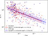 |
Fig. 5. Width of the radio profile plotted against the spin period, P, of the radio-detected pulsars in the simulation along with the observations. |
4.2. Companion
Since every pulsar in the simulation begins with a companion, it is instructive to investigate their eventual fate. The left panel of Fig. 6 shows the types of companions associated with NSs at the end of the simulation (noting that some NSs end up isolated). Most of the detected simulated systems end as isolated NSs or with a helium WD (HeWD) or carbon–oxygen WD (COWD) companion. Only a few systems retain other types of companions, such as non-degenerate stars, other NSs, oxygen–neon WDs (ONeWDs) or even a BH in some cases (although this simulation did not produce any BH companion). The right panel displays the initial companion mass as a function of the accretion duration. This plot informs us quite clearly that above an initial mass of 8 M⊙ for the companion, the survival of the binary is very rare. Most of the pulsars that end up isolated, had a companion whose initial mass was above 8 M⊙. Therefore, because of the supernova explosion, most of the time the binary is disrupted by the kick velocity of the companion at the remnant birth. This explains the rarity of NS-NS or NS-BH systems: their formation requires a companion with an initial mass above 8 M⊙, followed by a sufficiently low natal kick at the NS’s birth to prevent the binary from being disrupted.
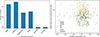 |
Fig. 6. Companion outcomes in the pulsar population. Left panel: Distribution of the type of the pulsars companions. HeWD stands for helium white dwarf, ‘isolated’ means the pulsar does not have a companion anymore, COWD stands for carbon-oxygen white dwarf, NotARemnant means the companion is a non-degenerate star, NS CCSN indicates an NS born after a core-collapse supernova, NS ECSN refers to an NS born after an electron capture supernova, and ONeWD stands for oxygen-neon white dwarf. Right panel: Initial mass of the pulsars’ companions plotted against the duration of the accretion phase, with the final type of the companion displayed. MS stands for main sequence star, and NS stands for NS. |
A further noticeable aspect of Fig. 6 is the fact that the initial mass of the companion is not correlated with the duration of the accretion phase of the binary. Basically, most of the binaries have an accretion phase which lasts between 108 and 109 yr. Furthermore, with Eq. (9b) we deduced a typical timescale of alignment for the rotation axis of the pulsar and the normal to the orbital plane,  :
:
 (32)
(32)
where n1 is the accretion torque, I is the moment of inertia, and Ω is the frequency of rotation of the pulsar. If we compute this timescale with MNS = 1.4 M⊙, ṀNS = 10−9 M⊙.yr−1, R = 12 km, B = 5 × 10⁶ T, Ω = 1 rad.s−1, and I = 1038 kg.m2, which are typical values for a pulsar that has been spinning down for a long time without accretion, it gives  kyr. Even if we change these values, in many cases, the typical duration of spin-orbit alignment is going to be lower than the typical duration of accretion, meaning most of the population has its spin-orbit aligned. Indeed, we already showed these results in Lorange et al. (2026, see Fig. 7), corresponding to ∼80% of the population with the spin-orbit angle, α, that is less than 10°. This supported the possibility of detecting pulsars with a misaligned spin-orbit (even though simulations show that such cases are relatively rare), as this study specifically investigated the spin-orbit alignment hypothesis.
4.3. Distribution of NS masses
Studying the mass that NSs can reach is very important in order to constrain the equation of state (EoS; Özel & Freire 2016). In this work we are able to follow the mass evolution of the NSs, and especially look at what is the distribution of mass characterising the recycled pulsars detected in the simulation. In Fig. 7, the PDF of the detected pulsar mass obtained in the simulation is represented. Linares (2020) gives a review of the NS mass distribution observed. An histogram including 44 mass measurements of pulsars was shown (Fig. 4 of Linares 2020), and at that time it was very new to obtain measurements of pulsars with masses greater than 2 M⊙, and for most of them they were spiders system. To this day, the number of measurements of mass of pulsars did not increase much6. Nevertheless, many of the observed mass measurements correspond to young pulsars, which clearly did not have time to undergo recycling. Moreover, the total number of available measurements remains limited. In contrast, in this type of simulation, we can obtain the mass of each recycled pulsar. The results suggest that due to accretion, the mass distribution of recycled pulsar is centred around 1.8 M⊙, with pulsars potentially reaching up to 2.7 M⊙. This is consistent with recent mass measurements of spider pulsars mentioned earlier. Therefore, the simulation indicates that if more masses of recycled NSs were measured, we could expect to find significantly more high masses compared to normal pulsars. Although the maximum NS mass imposed in SEVN was 3 M⊙, no pulsar in the simulation reached this value. There is also the possibility that the pulsars in the simulation accrete too much matter, as we did not observe many high-mass pulsars. Therefore, to diminish the accretion in the simulation, it would require larger τd so that the magnetic field could decay more slowly. This, in turn, would increase the inner disc radius rin for a longer period, thereby shortening the accretion phase. We tested this hypothesis in the simulation, but it failed to reproduce a realistic P−Ṗ diagram, making this scenario unlikely. Besides, as already mentioned, the number of measured masses of NSs is small (< 100). Overall, this study supports the recent high mass measurements of spider pulsars and suggests that the maximum mass of NSs may be higher than the 2.28 M⊙ proposed by Ruiz et al. (2018); otherwise, the model would not allow the P−Ṗ diagram to be reproduced so well.
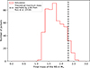 |
Fig. 7. Histogram of the final mass of the recycled pulsars in the simulation. The vertical dashed black line represents the theoretical maximum mass reachable by an NS from the study of Ruiz et al. (2018). |
4.4. Spatial distribution
Very interesting result concerns Fig. 8, where we can see the distributions in Galactic coordinates for the detected pulsars in the simulations and in the observations. It is striking that we recover well the positions of the observed pulsars with our simulations. However, we detected more pulsars especially at latitudes between −15° and 15° in the simulation. Therefore, we could expect many unidentified sources of 4FGL to lie at these latitudes. Furthermore, regarding the measured positions, there are uncertainties which can be greater than 20% on their measurement (Verbiest et al. 2012; Igoshev et al. 2016; Yao et al. 2017), which one must have in mind while comparing the simulated and observed positions of pulsars. In addition, this simulation can give us an estimation of the number of recycled pulsars born in the Galactic field which end up in the Galactic centre. Two majors hypothesis exist regarding the origin of the GeV excess. Either it is of a self-annihilating dark matter particle origin (Calore et al. 2015; Ackermann et al. 2017; Hooper 2022), or it is of pulsar origin (Yang & Aharonian 2016; Malyshev 2024; Sautron et al. 2024). Moreover Yang & Aharonian (2016) computed a total luminosity of 1030 W on the inner 10° ×10° region of the Galactic centre, which corresponds to a projected square of 1.4 kpc × 1.4 kpc around the Galactic centre (assuming a distance of 8.5 kpc from the Sun), i.e. a radial extent of ∼0.7 kpc. In the simulations, it would correspond to a total of ∼4.6 × 1028 W generated by ∼190 γ-ray pulsars on average in a 0.7 kpc radius from the Galactic centre (whether these pulsars are detected or not, and usually there is between 0 and 2 γ-ray detection in that area in the simulations). Therefore, the simulation hint to the fact that MSPs that were originally born in the Galactic field seem to only contribute to ∼5% of the GeV excess. In addition, Sautron et al. (2024) also found that young γ-ray pulsars could contribute to this excess with their detection prospects, and we discuss also the detection prospects of the recycled pulsars in Sect. 5.
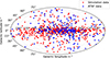 |
Fig. 8. Distribution in Galactic coordinates of the detected recycled pulsars in the simulations along with the observations. |
4.5. Geometry
Examining the geometry of the pulsars detected in various wavelengths is interesting. Indeed, Fig. 9 shows the viewing angle, ζ, as a function of the inclination angle, χ for each detected pulsar in the simulation. Although these angles are generated between 0 and 180°, we folded them between 0 and 90°. Basically, we retrieve an area of detection slightly different for radio pulsars compared to Johnston et al. (2020) where they studied the normal pulsars, but almost the same area of detection for γ-ray pulsars. The radio pulsars are detected along a region much broader than along the ζ = χ diagonal as it was the case for normal pulsars, the pulsars in γ-ray surveys only are seen above the line of equation ζ = 90 − χ, and the pulsars detected in both radio and γ-ray surveys are the intersection of these two areas. The area of radio detection is broader for recycled pulsars compared to normal pulsars, because recycled pulsars have larger ρ in general, which broaden the area of detection |ζ − χ|≤ρ (or |ζ − (π − χ)| ≤ ρ). We remind that ∼71 % of the pulsars in γ-ray surveys only have a radio flux above 30 μJy and a geometry favorable for a radio detection. Thus many of them would still be seen with a follow-up observation in radio. One can notice that it seems particularly difficult to see a pulsar with a rotation axis and magnetic axis aligned, i.e. χ ≈ 0°. Indeed, for γ-ray detection, the condition |ζ − π/2|≤χ is needed, and below χ = 20°, it almost never happens. The rarity of low detected χ values appears to be due to the fact that, as shown in Yang & Li (2023), the effect of accretion tends to lead to a misalignment between the rotation axis and the magnetic axis, i.e. having χ increasing towards 90°. Therefore, after accretion, since the magnetic field is weaker, the torque n3 caused by loss of energy via radiation of the pulsar has more difficulties to get χ to decrease. Furthermore, it is also plausible for those which get low χ that it took too much time and they became not luminous enough to be seen. These findings on the simulated population reflect well the observed values for ζ and χ. For instance Benli et al. (2021) constrained these angles for 10 radio-loud γ-ray MSPs, and found out that for both angles they are usually above 45°, and it is true that in our simulation the radio-loud γ-ray pulsars also verify this. Another example is the study of Guillemot & Tauris (2014), where they concluded that γ-ray energetic nearby MSPs are not seen because of their unfavorable viewing conditions, i.e. low ζ and we also see that high ζ are more favorable conditions of observations.
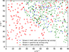 |
Fig. 9. Viewing angle (ζ) plotted against the inclination angle (χ) for the detected pulsars in the simulation. |
4.6. Spider population
We may ask whether, at the end of the simulation, it is possible to identify spider pulsars within the recycled population. A key process governing the evolution of spider systems is the irradiation of the donor star by the pulsar wind as demonstrated in the works of Chen et al. (2013), Benvenuto et al. (2014), Misra et al. (2025). In particular, companions with masses between 0.1 and 1 M⊙ can lose a significant fraction of their mass, causing the orbital period to first decrease and then increase again after a few Gyr (see Fig. 3 of Benvenuto et al. 2014, Figs. 1–4 of Chen et al. 2013, and Fig. 1 of Misra et al. 2025). We modelled this effect using the following equation:
 (33)
(33)
Indeed, the irradiation allows a mass loss Ṁc,evap from the companion, which depends on the escape velocity from the companion star surface vc, esc, its radius Rc, the semi-major axis of the binary a, the pulsar spin-down luminosity Lsp and the efficiency parameter fevap measuring how effectively the pulsar’s spin-down luminosity is converted into an evaporative wind. For our simulations we set fevap = 0.05, as having greater values seem to make difficult the production of black widows systems (Chen et al. 2013). A typical diagnostic to distinguish redbacks (RBs) from black widows (BWs) is a plot of the binary orbital period (Porb) versus the pulsar’s companion mass in M⊙, as in the right panel of Fig. 10 with the observed systems (see also Fig. 1 of Blanchard et al. 2025). In Fig. 10, the left panel shows this diagram for the entire simulated population, while the right panel presents the same plot restricted to the detected systems in the simulation and observed systems. RBs are located in the upper right, and BWs appear in the left region of the plot. To compute Porb in the simulation, we used Kepler’s third law, which gives
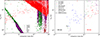 |
Fig. 10. Orbital period, Porb (in hr), as a function of companion mass (in M⊙). AGB stands for a companion that is on the asymptotic giant branch. Left panel: Entire simulated population. Right panel: Only systems with a detected pulsar by the pipeline in the simulation and observed systems. The companion mass reported is the median mass available in the ATNF catalogue for the observed systems. ‘Unknown (obs)’ means the pulsar has a null value in the ATNF catalog concerning its companion, ‘Sim’ stands for simulated, and ‘Obs’ stands for observed. The simulated systems are represented by squares and observed systems by circles. The different colours are for the different companions and are shown in the legend. |
 (34)
(34)
where Mc is the companion’s mass, MNS is the NS mass, a is the semi major axis of the binary and G is the gravitational constant. As a consequence, in a log-log plot of Porb against Mc, a line with a −1/2 slope in the left panel for the BWs can be observed, as they also have a close orbit. Thus the dependence in a is diminished, which is contrary to the RBs that are in wider orbits. Observed RBs typically have main sequence companions. Observationally, there are 13 RB systems with a main-sequence companion, whereas our simulation produces nine such systems. We found slightly more pulsars in the RB region with COWD companions compared to the observations. Observed BWs have ultra-light companions, while most simulated systems in the BW region host either HeWDs or COWDs, suggesting that some of the companion of observed BWs could actually be HeWDs or COWDs, or we could discover such spiders. We also struggle to reproduce BWs systems with a Porb > 2 h, whereas, on the left panel, we can see that a few systems with the characteristics of BWs with Porb > 2 h are formed but not detected. In addition, there are currently around 32 confirmed RBs and 50 confirmed BWs (Koljonen & Linares 2025), whereas our simulation produces roughly three times fewer spider-like pulsars. These discrepancies may indicate that a refinement is necessary for the initial conditions concerning the semi-major axis a which determine the initial orbital period, or combining a different set of parameters for the efficiency parameter of irradiation fevap and the accretion efficiency fMT or even other parameters describing the binary evolution. It may also hints that these systems might often form through alternative channels, as proposed by Metzler & Wadiasingh (2025). These authors suggest that the ultra-light companions of spiders could form in high-metallicity accretion discs over timescales exceeding > 1 Gyr (Patruno & Kama 2017), through dynamical capture or exchange interactions in clusters (Sigurdsson et al. 2003), or, especially for BWs, by the accretion of an ultra-compact X-ray binary companion’s outer layers onto the NS (Bailes et al. 2011). The study by Misra et al. (2025), which uses the detailed stellar evolution code MESA to characterise the spider population, shows that an accretion efficiency of 0.7 works better to reproduce the observed systems. We did not find any major differences in terms of detections between a simulation with fMT = 0.7 or also by changing fevap = 0.5. In summary, the simulation successfully produces two distinct groups reminiscent of spiders, which is encouraging. However, it underestimates the total number of observable spider systems. Therefore, including the additional formation channels mentioned above and fine-tuning the parameters related to binary evolution would likely lead to a better agreement with observed populations.
4.7. AIC scenario
Another formation channel for pulsars is the accretion-induced collapse (AIC) of WDs (Wang & Gong 2023). We performed a simulation starting with one million binary systems composed of an ONeWD and a main sequence companion, with the latter at a random evolutionary stage (0–100% of its main sequence lifetime), as was done for the pulsars in this study. We considered only ONeWDs, as their higher mass and composition make them ideal candidates for electron-capture supernovae. Consequently, most of the evolutionary channels leading to AIC involve an ONeWD (Wang & Liu 2020). Additional simulations were conducted with an initial population consisting of one third of each WD type, and only the ONeWDs were found to undergo collapse into NSs. The initial mass distributions for the WDs were taken from Tremblay et al. (2016). Figure 11 shows the resulting P–Ṗ diagram: the left panel displays the entire population of NSs formed via AIC, while the right panel presents only those that are detectable (either in radio or γ-rays) based on our detection pipeline, alongside the observed pulsar population. Out of the one million initial systems, ∼9000 WDs evolved into NSs (∼0.9%). Within the total population, we distinguish two main groups: one consists of NSs that accreted little mass and remain relatively young, behaving like “normal” pulsars; the other group lies in the region of mildly recycled pulsars (those with 30 ≤ P ≤ 1000 ms and Ṗ < 10−16 s/s), having accreted significantly more mass and consequently spun up to shorter periods, although it was not sufficient for them to become fully recycled as MSPs. After applying the detection pipeline, only ∼600 pulsars remain. Most of these belong to the normal pulsar population. A few objects (∼70) are found in the mildly recycled region of the P–Ṗ diagram, but they exhibit relatively high spin periods, with none below 20 ms. This suggests that a non-negligible fraction of recycled pulsars with relatively high spin periods may originate from the AIC of ONeWDs (depending on the birth rates of these objects). As shown in Fig. 3, these long-period/mildly recycled pulsars are not fully accounted for by the formation channel involving an NS formed via core-collapse supernova that later accretes mass from a companion. This discrepancy explains the imperfect agreement of our KS test for the radio population. The existence of this alternative formation pathway could help alleviate the so-called birth rate problem (Gençali & Ertan 2024), in which the Galactic core-collapse supernova rate appears to be lower than the combined estimated birth rates of NSs. In summary, this informs that among the whole ONeWDs simulated, ∼0.9% collapse into NSs, ∼6.9% are detectable and then ∼12.2% are in the area of mildly recycled pulsars considered in this work. Therefore, ∼7.6 × 10⁻³% of ONeWD (that were in a binary system) seem to contribute to the population of mildly recycled pulsars. The contribution of ONeWDs to the pulsar population could be explored in depth in future work, as it would require knowledge of the birth rate of ONeWDs, a quantity that remains highly uncertain.
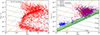 |
Fig. 11. Diagram of P−Ṗ of pulsars born after the AIC of WDs. Left panel: Entire simulated population. Right panel: Only systems with a detected pulsar by the pipeline along with the observations. |
It was suggested in Tauris et al. (2013) that the observed pulsars located in region II of the Corbet diagram (Fig. 12) may originate from AIC. In Fig. 12, the recycled pulsars originating from an AIC channel are shown as red circles with black outlines, whereas the other points correspond to recycled pulsars formed through core-collapse supernovae, paired either with a HeWD or a COWD companion. In our simulation, all pulsars formed through AIC indeed end up in region II. However, we also produce pulsars in region II that do not have an AIC origin. Therefore, while identifying an observed system as AIC-formed would imply that it should lie in region II, the reverse is not true: a system found in region II does not necessarily result from AIC. That said, if a system has Porb < 1 day and a P > 10 ms, an AIC origin appears significantly more likely.
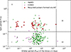 |
Fig. 12. Spin period (P) plotted against the orbital period (Porb) of the simulated pulsars. The red circles with a black outline are the AIC WD that became recycled pulsars, while the other points represents recycled pulsars formed via core-collapse supernova with either a HeWD or COWD companion. The four regions, labelled I, II, III, and IV, represent the same cut as in Tauris et al. (2013) to explain their differences as an evolutionary point of view. |
5. Discussion
5.1. Model evaluation and caveats
The model we used seems to reproduce the recycled pulsars in the radio and γ-ray wavelengths. However, it is important to address several points. A crucial aspect of the model is the mass transfer. Changing the accretion efficiency, fMT, was not explored in this work, and we decided to keep the value proposed by SEVN and used in other similar works (Bouffanais et al. 2021; Iorio et al. 2023). Nevertheless, changing this value would clearly impose a change on some parameters, such as τd and the birth rate.
Furthermore, SEVN does not allow spin-up during the CE phase. Therefore, this is a channel of formation of recycled pulsars from which we do not evaluate the contribution. However, Osłowski et al. (2011) estimated that the accreted matter during the CE phase would be too chaotic to produce spin-up and it could only decay the magnetic field. We also do not take into account the possible accretion from winds. Kiel et al. (2008) estimated that the spin-up caused by wind would also be too chaotic to produce any significant spin-up.
Still regarding the CE phase, major uncertainties remain about its treatment in binary evolution (Tauris & van den Heuvel 2023), particularly for the formation of double neutron star (DNS) or neutron star–black–hole (NS+BH) systems. When the donor star fills its Roche lobe, a CE phase is triggered with the NS, leading to a strong reduction of the orbital separation before the donor undergoes its supernova explosion. Moreover, Kruckow et al. (2016) showed that an in-spiraling NS can in principle eject the envelope of its companion, but that predicting the final post-CE separation remains highly uncertain. As long as dedicated studies do not clarify the CE evolution for such systems, accurately reproducing the number of observed DNS and NS+BH will remain challenging. In our simulations, we form about ∼2 − 5 DNS or NS+BH systems, while observations report 12 DNS systems. Despite these uncertainties, our models are still able to produce a fraction of the observed population. However, the small number of systems involved implies that the statistical significance remains limited.
The parameter ϵ characterising the ellipticity of the NS could also be an interesting parameter to vary in order to explore the possibility of the formation of sub-MSPs (Haensel & Zdunik 1989). In this work, we only tried to draw this parameter from a uniform distribution between the minimum and maximum value of ϵ hypothesised by Giliberti & Cambiotti (2022). The works of Bildsten (1998), Chakrabarty et al. (2003) indeed suggested that GW radiation allows the spin period P to remain above the millisecond threshold. Therefore, giving the same ϵ to every NS in the simulation and trying to find the value to obtain sub-MSPs could be quite interesting. Everything that is mentioned above could be explored in future works.
Part of the angular momentum of the binary is lost through magnetic braking, and one as to know that we used the formula proposed by Rappaport et al. (1983) for this phenomenon as it is implemented by default in SEVN. However, recently Chen et al. (2021) showed that using the prescription of Van et al. (2019) of magnetic braking could, among other things, influence a lot the number of NS + WD systems. Thus, in the future, it would also be interesting to evaluate the influence on the population while modifying the magnetic braking model of the binary.
For the simulation involving ONeWDs and main sequence stars, we adopted the same initial distributions for eccentricity (e) and mass ratio (q) as used for massive binaries, as described in Sect. 2. We also explored alternative power-law indices for the q distribution, varying it between −0.5 and 0.5 instead of the default −0.1, but found no significant impact on the simulation outcomes. Similarly, due to the lack of reliable constraints on the birth eccentricity distribution for low-mass binaries, we tested different power-law indices for e as well, and again observed negligible differences in the results.
Let us mention several geometrical or physical limitations concerning the striped wind model, which may affect our results. For instance, as suggested by Kalapotharakos et al. (2022), a more accurate description of the γ-ray luminosity might involve an additional parameter, such as the cut-off energy, and a different dependence on B and P, or equivalently on P and Ṗ, than the one assumed in (29). Moreover, plasma recollimation effects within the striped wind could reduce the γ-ray beam opening angle compared to the adopted value, leading to a smaller number of detectable pulsars.
5.2. Comparison with other works
Recently, Tabassum & Lorimer (2025) investigated the populations of both normal pulsars and MSPs in the radio and γ-ray bands. Their study focused in particular on testing various γ-ray luminosity models, leading them to rule out three of them–namely, the pair-starved polar cap (PSPC), the slot gap two-pole caustic (TPC), and the outer gap (OG) models–because they overproduced detectable pulsars. However, their overall modelling framework differs significantly from ours: they do not simulate the full accretion process, they do not include magnetic field decay, and they assume an exponential decay of the inclination angle χ (referred to as α in their work). Moreover, when they adopt the same γ-ray luminosity prescription as in this study, they do not incorporate the striped wind geometry. As a result, their model predicts a much larger number of detectable γ-ray sources, ranging from 350 up to 650. In contrast, our more comprehensive approach, which includes magnetic field decay, accretion history, and the striped wind geometry, yields a tighter prediction, with between 290 and 330 detectable γ-ray recycled pulsars, reflecting stochastic variations across simulation realisations. This results in fewer than ∼220 unidentified sources in the 4FGL catalog, significantly narrowing the allowed range compared to the upper limit of ∼520 unidentified sources predicted by Tabassum & Lorimer (2025).
Gonthier et al. (2018) estimated that approximately 11 000 MSPs would be required within the inner Galactic centre (defined as the 7° ×7° region of interest, corresponding to a radius of about 0.5 kpc) to account for the GeV excess. Their scenario relies on the contribution of GCs that have migrated into the Galactic bulge through dynamical friction (Gnedin et al. 2014). In contrast, our study considers only pulsars formed in the Galactic spiral arms. These tend to be more luminous than those assumed by Gonthier et al. (2018). Nevertheless, our results indicate that only about 190 MSPs born in the spiral arms contribute to roughly 5% of the GeV excess. Therefore, if the GeV excess is entirely due to pulsars, it is still entirely plausible that a much larger population of MSPs originating from GCs resides in the Galactic centre as estimated by Gonthier et al. (2018) or they were born in the bulge, but they are beyond current detectability.
The studies of Kiel et al. (2008), Kiel & Hurley (2009) were among the first to attempt reproducing the pulsar population by accounting for the full evolutionary path of NSs in binary systems. However, several key differences exist between their approach and ours. First, their magnetic field decay prescription is exponential; thus, if they had used the same decay timescales τd as those identified in our work (0.05, 1.4, or 2.3 Myr), the magnetic fields of their NSs would decay unrealistically fast. As a result, they require significantly higher values of τd to reproduce the observed population. Secondly, the equation they adopt for the evolution of the angular velocity Ω is much simpler than the one used in this study, which incorporates several additional physical effects. Furthermore, while our initial distributions for P0 and B0 are informed by observational constraints and recent population synthesis efforts (Igoshev et al. 2022; Sautron et al. 2024), their work relies on uniform distributions for these parameters, not grounded in observational data or detailed modelling. Finally, their comparison with observations is limited, as their population synthesis framework does not include a detection model to account for selection effects.
As mentioned in Sect. 2, we obtained matching P−Ṗ diagrams from the observations and simulations for a number of simulated binaries between 4.6 × 10⁵ and 5.7 × 10⁵, corresponding to a birth rate between 3.3 − 4.1 × 10⁻⁶ yr−1. Studies by Story et al. (2007) and Gonthier et al. (2018) found the birth rate of MSPs to be in the range of 3 − 6.5 × 10⁻⁶ yr−1. The birth rate found in our study is consistent with the findings of Story et al. (2007) and Gonthier et al. (2018). We constrain the birth rate of recycled pulsars even more with this work.
5.3. Detection prospects
We wanted to assess the detectability of new recycled pulsars sources with this model. To do so, we considered the survey parameters of SKA. See Appendix D to see the parameters and in order to make predictions for radio observations. Moreover, concerning the γ-ray wavelengths, we took into account an instrument that would be ten times more sensitive than Fermi/LAT (i.e. we adopted a detection threshold of Flim = 1 × 10⁻¹⁶ W.m−2, as the average flux limit of ∼1 × 10⁻¹⁵ W.m−2 was derived from the Fermi/LAT all-sky sensitivity map). These considerations allowed us to multiply the number of radio detections by approximately three and the number of γ-ray detections by about five. This improvement in sensitivity also allowed us to detect around ten γ-ray pulsars in the Galactic centre, indicating that an even higher sensitivity would be necessary to uncover additional pulsars in the Galactic centre.
6. Conclusions
This study is the first ever to evolve the population of pulsars in binary systems in a complete way by taking into account the binary processes. By doing so, we also took into account the observational biases from radio and γ-ray surveys in order to analyse the recycled pulsar population.
We showed that our model reproduces most of the recycled pulsar population in the radio and γ-ray wavelengths and that most of the mildly recycled pulsars (those with 30 ≤ P ≤ 1000 ms and Ṗ < 10−16 s/s) seem to originate from the AIC of WDs. In order to reproduce the population, the characteristic B-field decay timescale, τd, was chosen to be 0.05, 1.4, or 2.3 Myr, with most of the population evolving with τd = 0.05 Myr. Moreover, with this model we estimate a birth rate for recycled pulsars between (3.3–4.1) × 10−6 yr−1. The striped wind model allowed us to reproduce the gamma-ray peak separation observed for γ-ray recycled pulsars very well. Most of the pulsars accrete for 108 − 9 yr no matter the type or initial mass of the companion. Since the timescale for alignment between the rotation axis of the NS and the normal of the orbital plane is often short, we obtained ∼80% of the population that has these two axes aligned (Lorange et al. 2026). Moreover, the mean mass obtained for this population is about 1.8 M⊙, with some very high mass pulsars, up to 2.7 M⊙. The mean mass is in agreement with the recent measurements of high masses of pulsars in spider systems (e.g. Linares 2020). Furthermore, in the simulation we were able to recover pulsars that have the characteristics of spiders but not the whole observed population, indicating that other channels of formation (in addition to the one considered in this work) must be at work to obtain spiders. Moreover, to obtain a more similar population of spiders, as suggested by Misra et al. (2025), it is likely necessary for a fraction of the population to have a higher accretion efficiency. The positions of the detected recycled pulsars in the simulation are generally well reproduced, although the simulation predicts more pulsars between latitudes −15° and 15° than observed. We estimate that MSPs formed in the Galactic field contribute only to ∼5% of the γ-ray galactic center excess, corresponding to roughly 190 MSPs in the Galactic centre. This result suggests that if the γ-ray galactic center excess originates only from pulsars, the majority of MSPs in the Galactic centre likely come from GCs that migrated inwards through dynamical friction or they were born in the bulge. Either way, we are not able to detect them today (Gnedin et al. 2014; Gonthier et al. 2018). Finally, most of the detected pulsars seem to have an inclination angle, χ, greater than 10°, and it also seems easier to observe pulsars that have a viewing angle, ζ, greater than 45°, which has been supported by other studies (Benli et al. 2021; Guillemot & Tauris 2014). We were also able to make some predictions: We expect approximately three times more radio recycled pulsars thanks to SKA and about five times more detections of γ-ray recycled pulsars with an instrument that has a sensitivity increased by one order of magnitude compared to Fermi/LAT.
Other interesting topics to explore include adding another channel of formation for recycled pulsars; studying the contribution of AIC ONeWD to the population of pulsars in depth; adding the possible ablation of the companion by the pulsar to study the spiders; and evaluating the detectability of continuous GWs from the recycled population, as was already done for the normal population by Cieślar et al. (2021). In addition, more constraints could be found about the numerous parameters of the model while focusing on a restricted number of parameters.
Acknowledgments
This work has been supported by the French Research Agency grant ANR-20-CE31-0010. We would like to thank Francesca Calore, Joanna Berteaud and Maïca Clavel for insightful discussions. D.M. acknowledges the support of the Department of Atomic Energy, Government of India, under project No. 12-R&D-TFR-5.02-0700. We also thank the anonymous referee for the helpful comments and suggestions, which helped improve the paper.
References
- Abdo, A. A., Ajello, M., Allafort, A., et al. 2013, ApJS, 208, 17 [Google Scholar]
- Abdollahi, S., Acero, F., Baldini, L., et al. 2022, ApJS, 260, 53 [NASA ADS] [CrossRef] [Google Scholar]
- Abolmasov, P., Biryukov, A., & Popov, S. B. 2024, Galaxies, 12, 7 [NASA ADS] [CrossRef] [Google Scholar]
- Ackermann, M., Ajello, M., Albert, A., et al. 2017, ApJ, 840, 43 [NASA ADS] [CrossRef] [Google Scholar]
- Alpar, M. A., Cheng, A. F., Ruderman, M. A., & Shaham, J. 1982, Nature, 300, 728 [NASA ADS] [CrossRef] [Google Scholar]
- Backer, D. C., Kulkarni, S. R., Heiles, C., Davis, M. M., & Goss, W. M. 1982, Nature, 300, 615 [NASA ADS] [CrossRef] [Google Scholar]
- Bailes, M., Bates, S. D., Bhalerao, V., et al. 2011, Science, 333, 1717 [NASA ADS] [CrossRef] [Google Scholar]
- Bailes, M., Jameson, A., Abbate, F., et al. 2020, PASA, 37, e028 [NASA ADS] [CrossRef] [Google Scholar]
- Bates, S. D., Lorimer, D. R., Rane, A., & Swiggum, J. 2014, MNRAS, 439, 2893 [NASA ADS] [CrossRef] [Google Scholar]
- Belczynski, K., & Taam, R. E. 2008, ApJ, 685, 400 [NASA ADS] [CrossRef] [Google Scholar]
- Beniamini, P., Hotokezaka, K., van der Horst, A., & Kouveliotou, C. 2019, MNRAS, 487, 1426 [NASA ADS] [CrossRef] [Google Scholar]
- Benli, O., Pétri, J., & Mitra, D. 2021, A&A, 647, A101 [NASA ADS] [CrossRef] [EDP Sciences] [Google Scholar]
- Benvenuto, O. G., De Vito, M. A., & Horvath, J. E. 2014, ApJ, 786, L7 [NASA ADS] [CrossRef] [Google Scholar]
- Berteaud, J., Eckner, C., Calore, F., Clavel, M., & Haggard, D. 2024, ApJ, 974, 144 [Google Scholar]
- Bessolaz, N., Zanni, C., Ferreira, J., Keppens, R., & Bouvier, J. 2008, A&A, 478, 155 [NASA ADS] [CrossRef] [EDP Sciences] [Google Scholar]
- Bhattacharya, D., & van den Heuvel, E. P. J. 1991, Phys. Rep., 203, 1 [Google Scholar]
- Bhattacharya, D., Wijers, R. A. M. J., Hartman, J. W., & Verbunt, F. 1992, A&A, 254, 198 [NASA ADS] [Google Scholar]
- Bildsten, L. 1998, ApJ, 501, L89 [Google Scholar]
- Biryukov, A., & Abolmasov, P. 2021, MNRAS, 505, 1775 [NASA ADS] [CrossRef] [Google Scholar]
- Blanchard, C., Guillemot, L., Voisin, G., Cognard, I., & Theureau, G. 2025, A&A, 698, A239 [NASA ADS] [CrossRef] [EDP Sciences] [Google Scholar]
- Bouffanais, Y., Mapelli, M., Santoliquido, F., et al. 2021, MNRAS, 505, 3873 [NASA ADS] [CrossRef] [Google Scholar]
- Calore, F., Cholis, I., & Weniger, C. 2015, JCAP, 2015, 038 [Google Scholar]
- Cameron, A. D., Champion, D. J., Bailes, M., et al. 2020, MNRAS, 493, 1063 [NASA ADS] [CrossRef] [Google Scholar]
- Carilli, C. L., & Rawlings, S. 2004, New Astron. Rev., 48, 979 [Google Scholar]
- Chakrabarty, D., Morgan, E. H., Muno, M. P., et al. 2003, Nature, 424, 42 [CrossRef] [PubMed] [Google Scholar]
- Chamandy, L., Frank, A., Blackman, E. G., et al. 2018, MNRAS, 480, 1898 [NASA ADS] [CrossRef] [Google Scholar]
- Chattopadhyay, D., Stevenson, S., Hurley, J. R., Rossi, L. J., & Flynn, C. 2020, MNRAS, 494, 1587 [NASA ADS] [CrossRef] [Google Scholar]
- Chen, H.-L., Chen, X., Tauris, T. M., & Han, Z. 2013, ApJ, 775, 27 [NASA ADS] [CrossRef] [Google Scholar]
- Chen, H.-L., Tauris, T. M., Han, Z., & Chen, X. 2021, MNRAS, 503, 3540 [NASA ADS] [CrossRef] [Google Scholar]
- Cieślar, M., Bulik, T., Curyło, M., et al. 2021, A&A, 649, A92 [NASA ADS] [CrossRef] [EDP Sciences] [Google Scholar]
- Cordes, J. M., & McLaughlin, M. A. 2003, ApJ, 596, 1142 [NASA ADS] [CrossRef] [Google Scholar]
- Cordes, J. M., Freire, P. C. C., Lorimer, D. R., et al. 2006, ApJ, 637, 446 [NASA ADS] [CrossRef] [Google Scholar]
- Cranmer, K., Brehmer, J., & Louppe, G. 2020, Proc. Natl. Acad. Sci., 117, 30055 [Google Scholar]
- Cumming, A., Arras, P., & Zweibel, E. 2004, ApJ, 609, 999 [NASA ADS] [CrossRef] [Google Scholar]
- Dall’Osso, S., Granot, J., & Piran, T. 2012, MNRAS, 422, 2878 [CrossRef] [Google Scholar]
- Dirson, L., Pétri, J., & Mitra, D. 2022, A&A, 667, A82 [NASA ADS] [CrossRef] [EDP Sciences] [Google Scholar]
- Eggleton, P. P. 1983, ApJ, 268, 368 [Google Scholar]
- Faucher-Giguère, C.-A., & Kaspi, V. M. 2006, ApJ, 643, 332 [CrossRef] [Google Scholar]
- Fruchter, A. S., Stinebring, D. R., & Taylor, J. H. 1988, Nature, 333, 237 [Google Scholar]
- Gençali, A. A., & Ertan, Ü. 2024, MNRAS, 534, 1481 [Google Scholar]
- Giacobbo, N., & Mapelli, M. 2020, ApJ, 891, 141 [NASA ADS] [CrossRef] [Google Scholar]
- Giliberti, E., & Cambiotti, G. 2022, MNRAS, 511, 3365 [NASA ADS] [CrossRef] [Google Scholar]
- Gnedin, O. Y., Ostriker, J. P., & Tremaine, S. 2014, ApJ, 785, 71 [Google Scholar]
- Gonthier, P. L., Harding, A. K., Ferrara, E. C., et al. 2018, ApJ, 863, 199 [NASA ADS] [CrossRef] [Google Scholar]
- Grainge, K., Alachkar, B., Amy, S., et al. 2017, Astron. Rep., 61, 288 [NASA ADS] [CrossRef] [Google Scholar]
- Guillemot, L., & Tauris, T. M. 2014, MNRAS, 439, 2033 [NASA ADS] [CrossRef] [Google Scholar]
- Gullón, M., Miralles, J. A., Viganò, D., & Pons, J. A. 2014, MNRAS, 443, 1891 [CrossRef] [Google Scholar]
- Haensel, P., & Zdunik, J. L. 1989, Nature, 340, 617 [Google Scholar]
- Han, Z.-W., Ge, H.-W., Chen, X.-F., & Chen, H.-L. 2020, Res. Astron. Astrophys., 20, 161 [CrossRef] [Google Scholar]
- Han, J. L., Wang, C., Wang, P. F., et al. 2021, Res. Astron. Astrophys., 21, 107 [CrossRef] [Google Scholar]
- Haslam, C. G. T., Salter, C. J., Stoffel, H., & Wilson, W. E. 1982, A&AS, 47, 1 [NASA ADS] [Google Scholar]
- Hooper, D. 2022, arXiv e-prints [arXiv:2209.14370] [Google Scholar]
- Hurley, J. R., Tout, C. A., & Pols, O. R. 2002, MNRAS, 329, 897 [Google Scholar]
- Igoshev, A. P., & Popov, S. B. 2024, MNRAS, 535, L54 [Google Scholar]
- Igoshev, A., Verbunt, F., & Cator, E. 2016, A&A, 591, A123 [NASA ADS] [CrossRef] [EDP Sciences] [Google Scholar]
- Igoshev, A. P., Frantsuzova, A., Gourgouliatos, K. N., et al. 2022, MNRAS, 514, 4606 [CrossRef] [Google Scholar]
- Iorio, G., Mapelli, M., Costa, G., et al. 2023, MNRAS, 524, 426 [NASA ADS] [CrossRef] [Google Scholar]
- Jawor, J. A., & Tauris, T. M. 2022, MNRAS, 509, 634 [Google Scholar]
- Johnston, S., & Karastergiou, A. 2017, MNRAS, 467, 3493 [CrossRef] [Google Scholar]
- Johnston, S., & Karastergiou, A. 2019, MNRAS, 485, 640 [NASA ADS] [CrossRef] [Google Scholar]
- Johnston, S., Lyne, A. G., Manchester, R. N., et al. 1992, MNRAS, 255, 401 [Google Scholar]
- Johnston, S., Smith, D. A., Karastergiou, A., & Kramer, M. 2020, MNRAS, 497, 1957 [NASA ADS] [CrossRef] [Google Scholar]
- Johnston, S., Kramer, M., Karastergiou, A., et al. 2023, MNRAS, 520, 4801 [Google Scholar]
- Kalapotharakos, C., Harding, A. K., Kazanas, D., & Wadiasingh, Z. 2019, ApJ, 883, L4 [NASA ADS] [CrossRef] [Google Scholar]
- Kalapotharakos, C., Wadiasingh, Z., Harding, A. K., & Kazanas, D. 2022, ApJ, 934, 65 [NASA ADS] [CrossRef] [Google Scholar]
- Kiel, P. D., & Hurley, J. R. 2009, MNRAS, 395, 2326 [NASA ADS] [CrossRef] [Google Scholar]
- Kiel, P. D., Hurley, J. R., Bailes, M., & Murray, J. R. 2008, MNRAS, 388, 393 [NASA ADS] [CrossRef] [Google Scholar]
- Kijak, J., & Gil, J. 1998, MNRAS, 299, 855 [NASA ADS] [CrossRef] [Google Scholar]
- Kijak, J., & Gil, J. 2003, A&A, 397, 969 [NASA ADS] [CrossRef] [EDP Sciences] [Google Scholar]
- Koljonen, K. I. I., & Linares, M. 2025, ApJ, 994, 8 [Google Scholar]
- Kramer, M., & Stappers, B. 2015, in Advancing Astrophysics with the Square Kilometre Array (AASKA14), 36 [Google Scholar]
- Kramer, M., Bell, J. F., Manchester, R. N., et al. 2003, MNRAS, 342, 1299 [NASA ADS] [CrossRef] [Google Scholar]
- Krishnakumar, M. A., Mitra, D., Naidu, A., Joshi, B. C., & Manoharan, P. K. 2015, ApJ, 804, 23 [NASA ADS] [CrossRef] [Google Scholar]
- Kroupa, P. 2001, MNRAS, 322, 231 [NASA ADS] [CrossRef] [Google Scholar]
- Kruckow, M. U., Tauris, T. M., Langer, N., et al. 2016, A&A, 596, A58 [NASA ADS] [CrossRef] [EDP Sciences] [Google Scholar]
- Linares, M. 2020, in Multifrequency Behaviour of High Energy Cosmic Sources – XIII. 3–8 June 2019. Palermo, 23 [Google Scholar]
- Lorange, A., Pétri, J., Sautron, M., & Vigon, V. 2026, A&A, in press, https://doi.org/10.1051/0004-6361/202556461 [Google Scholar]
- Lorimer, D. R., & Kramer, M. 2004, Handbook of Pulsar Astronomy (Cambridge University Press), 4 [Google Scholar]
- Lorimer, D. R., Stairs, I. H., Freire, P. C., et al. 2006, ApJ, 640, 428 [NASA ADS] [CrossRef] [Google Scholar]
- MacLeod, M., & Ramirez-Ruiz, E. 2015, ApJ, 798, L19 [Google Scholar]
- Malyshev, D. V. 2024, arXiv e-prints [arXiv:2406.03990] [Google Scholar]
- Manchester, R. N., Lyne, A. G., Camilo, F., et al. 2001, MNRAS, 328, 17 [NASA ADS] [CrossRef] [Google Scholar]
- Manchester, R. N., Hobbs, G. B., Teoh, A., & Hobbs, M. 2005, AJ, 129, 1993 [Google Scholar]
- Mapelli, M., Spera, M., Montanari, E., et al. 2020, ApJ, 888, 76 [NASA ADS] [CrossRef] [Google Scholar]
- Metzler, Z., & Wadiasingh, Z. 2025, ApJ, 992, 116 [Google Scholar]
- Misra, D., Linares, M., & Ye, C. S. 2025, A&A, 693, A314 [NASA ADS] [CrossRef] [EDP Sciences] [Google Scholar]
- Mitra, D. 2017, JApA, 38, 52 [NASA ADS] [Google Scholar]
- Mitra, D., Basu, R., Melikidze, G. I., & Arjunwadkar, M. 2020, MNRAS, 492, 2468 [NASA ADS] [CrossRef] [Google Scholar]
- Miyamoto, M., & Nagai, R. 1975, PASJ, 27, 533 [NASA ADS] [Google Scholar]
- Navarro, J. F., Frenk, C. S., & White, S. D. M. 1997, ApJ, 490, 493 [Google Scholar]
- Omelyan, I. P., Mryglod, I. M., & Folk, R. 2002, Phys. Rev. E, 66, 026701 [Google Scholar]
- Osłowski, S., Bulik, T., Gondek-Rosińska, D., & Belczyński, K. 2011, MNRAS, 413, 461 [CrossRef] [Google Scholar]
- Özel, F., & Freire, P. 2016, ARA&A, 54, 401 [Google Scholar]
- Özel, F., Psaltis, D., Narayan, R., & Santos Villarreal, A. 2012, ApJ, 757, 55 [Google Scholar]
- Papitto, A., & de Martino, D. 2022, Astrophys. Space Sci. Lib., 465, 157 [NASA ADS] [CrossRef] [Google Scholar]
- Pardo-Araujo, C., Ronch, M., Graber, V., & Rea, N. 2025, A&A, 696, A114 [NASA ADS] [CrossRef] [EDP Sciences] [Google Scholar]
- Patruno, A., & Kama, M. 2017, A&A, 608, A147 [NASA ADS] [CrossRef] [EDP Sciences] [Google Scholar]
- Patruno, A., & Watts, A. L. 2021, Astrophys. Space Sci. Lib., 461, 143 [NASA ADS] [CrossRef] [Google Scholar]
- Payne, D. J. B., & Melatos, A. 2007, MNRAS, 376, 609 [Google Scholar]
- Peters, P. C. 1964, Phys. Rev., 136, B1224 [NASA ADS] [CrossRef] [Google Scholar]
- Pétri, J. 2011, MNRAS, 412, 1870 [Google Scholar]
- Pétri, J. 2026, A&A, 706, 215 [Google Scholar]
- Philippov, A., Tchekhovskoy, A., & Li, J. G. 2014, MNRAS, 441, 1879 [NASA ADS] [CrossRef] [Google Scholar]
- Qian, L., Yao, R., Sun, J., et al. 2020, Innovation, 1, 100053 [Google Scholar]
- Radhakrishnan, V., & Srinivasan, G. 1982, Curr. Sci., 51, 1096 [NASA ADS] [Google Scholar]
- Rappaport, S., Verbunt, F., & Joss, P. C. 1983, ApJ, 275, 713 [Google Scholar]
- Remazeilles, M., Dickinson, C., Banday, A. J., Bigot-Sazy, M. A., & Ghosh, T. 2015, MNRAS, 451, 4311 [NASA ADS] [CrossRef] [Google Scholar]
- Riess, A. G., Filippenko, A. V., Challis, P., et al. 1998, AJ, 116, 1009 [Google Scholar]
- Roberts, M. S. E. 2013, IAU Symp., 291, 127 [NASA ADS] [Google Scholar]
- Ruiz, M., Shapiro, S. L., & Tsokaros, A. 2018, Phys. Rev. D, 97, 021501 [NASA ADS] [CrossRef] [Google Scholar]
- Sana, H., de Mink, S. E., de Koter, A., et al. 2012, Science, 337, 444 [Google Scholar]
- Sautron, M., Pétri, J., Mitra, D., & Dirson, L. 2024, A&A, 691, A349 [NASA ADS] [CrossRef] [EDP Sciences] [Google Scholar]
- Sautron, M., McEwen, A. E., Younes, G., et al. 2025, ApJ, 986, 88 [Google Scholar]
- Sgalletta, C., Iorio, G., Mapelli, M., et al. 2023, MNRAS, 526, 2210 [NASA ADS] [CrossRef] [Google Scholar]
- Siegert, T. 2019, A&A, 632, L1 [NASA ADS] [CrossRef] [EDP Sciences] [Google Scholar]
- Sigurdsson, S., Richer, H. B., Hansen, B. M., Stairs, I. H., & Thorsett, S. E. 2003, Science, 301, 193 [NASA ADS] [CrossRef] [Google Scholar]
- Smirnov, N. V. 1948, Ann. Math. Stat., 19, 279 [CrossRef] [Google Scholar]
- Smith, D. A., Bruel, P., Cognard, I., et al. 2019, ApJ, 871, 78 [NASA ADS] [CrossRef] [Google Scholar]
- Smith, D. A., Abdollahi, S., Ajello, M., et al. 2023, ApJ, 958, 191 [NASA ADS] [CrossRef] [Google Scholar]
- Spera, M., & Mapelli, M. 2017, MNRAS, 470, 4739 [Google Scholar]
- Spera, M., Mapelli, M., Giacobbo, N., et al. 2019, MNRAS, 485, 889 [Google Scholar]
- Srinivasan, G. 1990, Adv. Space Res., 10, 167 [Google Scholar]
- Srinivasan, G., & van den Heuvel, E. P. J. 1982, A&A, 108, 143 [Google Scholar]
- Srinivasan, G., Bhattacharya, D., Muslimov, A. G., & Tsygan, A. J. 1990, Curr. Sci., 59, 31 [Google Scholar]
- Story, S. A., Gonthier, P. L., & Harding, A. K. 2007, ApJ, 671, 713 [Google Scholar]
- Sukhbold, T., Ertl, T., Woosley, S. E., Brown, J. M., & Janka, H.-T. 2016, ApJ, 821, 38 [Google Scholar]
- Tabassum, S., & Lorimer, D. R. 2025, ApJ, 988, 78 [Google Scholar]
- Tauris, T. M., & van den Heuvel, E. P. J. 2023, Physics of Binary Star Evolution. From Stars to X-ray Binaries and Gravitational Wave Sources (Princeton University Press) [Google Scholar]
- Tauris, T. M., Langer, N., & Kramer, M. 2012, MNRAS, 425, 1601 [NASA ADS] [CrossRef] [Google Scholar]
- Tauris, T. M., Sanyal, D., Yoon, S.-C., & Langer, N. 2013, A&A, 558, A39 [NASA ADS] [CrossRef] [EDP Sciences] [Google Scholar]
- Thompson, D. J. 2008, Rep. Progr. Phys., 71, 116901 [Google Scholar]
- Tremblay, P. E., Cummings, J., Kalirai, J. S., et al. 2016, MNRAS, 461, 2100 [NASA ADS] [CrossRef] [Google Scholar]
- Van, K. X., Ivanova, N., & Heinke, C. O. 2019, MNRAS, 483, 5595 [NASA ADS] [CrossRef] [Google Scholar]
- Verbiest, J. P. W., Weisberg, J. M., Chael, A. A., Lee, K. J., & Lorimer, D. R. 2012, ApJ, 755, 39 [NASA ADS] [CrossRef] [Google Scholar]
- Viganò, D., Rea, N., Pons, J. A., et al. 2013, MNRAS, 434, 123 [CrossRef] [Google Scholar]
- Wang, D., & Gong, B. P. 2023, MNRAS, 526, 5021 [Google Scholar]
- Wang, B., & Liu, D. 2020, Res. Astron. Astrophys., 20, 135 [CrossRef] [Google Scholar]
- Wang, J., Zhang, C. M., & Chang, H. K. 2012, A&A, 540, A100 [NASA ADS] [CrossRef] [EDP Sciences] [Google Scholar]
- Watters, K. P., Romani, R. W., Weltevrede, P., & Johnston, S. 2009, ApJ, 695, 1289 [Google Scholar]
- Weltevrede, P., & Johnston, S. 2008, MNRAS, 387, 1755 [Google Scholar]
- Wijnands, R., & van der Klis, M. 1998, Nature, 394, 344 [CrossRef] [Google Scholar]
- Wolszczan, A., & Frail, D. A. 1992, Nature, 355, 145 [CrossRef] [Google Scholar]
- Xilouris, K. M., Kramer, M., Jessner, A., et al. 1998, ApJ, 501, 286 [NASA ADS] [CrossRef] [Google Scholar]
- Yang, R.-Z., & Aharonian, F. 2016, A&A, 589, A117 [NASA ADS] [CrossRef] [EDP Sciences] [Google Scholar]
- Yang, H.-R., & Li, X.-D. 2023, ApJ, 945, 2 [Google Scholar]
- Yao, J. M., Manchester, R. N., & Wang, N. 2017, ApJ, 835, 29 [NASA ADS] [CrossRef] [Google Scholar]
- You, Z.-Q., Zhu, X., Liu, X., et al. 2025, Nat. Astron., 9, 552 [Google Scholar]
- Yusifov, I., & Küçük, I. 2004, A&A, 422, 545 [NASA ADS] [CrossRef] [EDP Sciences] [Google Scholar]
- Zhang, C. M., & Kojima, Y. 2006, MNRAS, 366, 137 [NASA ADS] [CrossRef] [Google Scholar]
Appendix A: Ratio of the pulsar’s radiation loss torque and the gravitational wave torque
In the set of differential equations that we use (Eqs. (9a) to (9c)), we take into account a torque, nGW, caused by GWs. However, this torque depends on Ω5. Therefore compared to the torque due to the pulsar’s radiation loss, n3 (which depends to Ω3), it can often be neglected. If we compute the ratio of both torques, we obtain
 (A.1)
(A.1)
To choose when to consider the torque caused by GWs, we look into when the ratio of Eq. (A.1) would be greater than 0.05. If we take B = 7 × 10⁴ T and ϵ = 10−7, it gives Ωlim ∼ 1100 rad.s−1, while actually most of the time ϵ can be lower than this, or the magnetic field a bit higher, resulting in higher Ωlim. Thus, to be very cautious and thorough, we even adopted Ωlim = 960 rad.s−1. Therefore in this work, we do not neglect the GWs torque for Ω ≥ Ωlim.
Appendix B: Influence of the ISM on the radio pulse profile
Dispersion and scattering caused by the ISM lead to a broader radio pulse profile. In order to determine the influence of the ISM through τDM, the formula of Bates et al. (2014) can be used,
 (B.1)
(B.1)
Here, e is the electron charge, me its mass, Δfch the width of frequency of the instrument channel in Hz, f the observing frequency in Hz, and DM the dispersion measure in pc/cm3. Furthermore, in order to determine the influence of scattering by an heterogeneous and turbulent ISM through τscat, the empirical fit relationship from Krishnakumar et al. (2015) is used
 (B.2)
(B.2)
Both τDM and τscat are given in units of second (s) and depend on the dispersion measure DM (in units of pc/cm3), which is found for each pulsar by running the code of Yao et al. (2017) converting the distance of a pulsar into the dispersion measure thanks to their state-of-the art model of the Galactic electron density distribution. See Table 1 for the parameters used for the two surveys considered, i.e. FAST GPPS and PMPS.
Appendix C: Anisotropy of the striped wind model
The link between the γ-ray flux and the total γ-ray luminosity is not a straightforward relation to deduce. The problem resides in the highly anisotropic emission pattern of the pulsar striped wind. This anisotropy is usually embedded in a so-called beaming factor, fΩ, describing the flux pattern depending on the obliquity χ and line of sight inclination ζ. Its definition is found in Watters et al. (2009), Pétri (2011, 2026) and shown on a log scale in fig. C.1 for the force-free dipole magnetosphere model. For high inclinations (ζ), it is about 0.2, whereas for low inclinations( ζ), it is very high, well above ten.
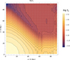 |
Fig. C.1. Flux anisotropy factor (fΩ; in log) for the striped wind model versus obliquity (χ) and inclination of Earth’s line of sight (ζ). |
Appendix D: SKA survey parameters
Table D.1 displays the SKA survey parameters in the mid-frequency ranges we used to make the predictions in Sect. 5.3. SKA is described in Carilli & Rawlings (2004), Kramer & Stappers (2015), Grainge et al. (2017). SKA-1-Mid represents the estimate of the initially planned SKA operation.
Survey parameters of SKA-1-Mid.
All Tables
All Figures
|
Fig. 1. Diagram of P−Ṗ of the observed pulsars considered in this work along with the death line (solid green line) and the death valley (shaded green area). |
| In the text | |
|
Fig. 2. Evolution in the P−Ṗ diagram of a pulsar in the simulation that becomes an MSP. |
| In the text | |
|
Fig. 3. Diagram of P−Ṗ for observed and simulated pulsars in different wavelengths. Left panel: P−Ṗ diagram for the detected pulsars in radio surveys only in the simulations in red along with the observations in radio for the FAST GPPS or PMPS survey in blue. Middle panel: P−Ṗ diagram for the detected pulsars in γ-ray surveys only in the simulations in green, along with the observed pulsars in γ-ray from Fermi surveys only in blue. Right panel: P−Ṗ diagram for the simulated pulsars detected both in radio and γ-ray surveys in purple, along with observations for the FAST GPPS or PMPS survey simultaneously with the γ-ray observations from Fermi in blue. For all the panels, the death line is represented as a green solid line, and the death valley is the shaded green area. |
| In the text | |
|
Fig. 4. Distribution of the γ-ray peak separation of the simulated population along with the observations from the 3PC catalogue. |
| In the text | |
|
Fig. 5. Width of the radio profile plotted against the spin period, P, of the radio-detected pulsars in the simulation along with the observations. |
| In the text | |
|
Fig. 6. Companion outcomes in the pulsar population. Left panel: Distribution of the type of the pulsars companions. HeWD stands for helium white dwarf, ‘isolated’ means the pulsar does not have a companion anymore, COWD stands for carbon-oxygen white dwarf, NotARemnant means the companion is a non-degenerate star, NS CCSN indicates an NS born after a core-collapse supernova, NS ECSN refers to an NS born after an electron capture supernova, and ONeWD stands for oxygen-neon white dwarf. Right panel: Initial mass of the pulsars’ companions plotted against the duration of the accretion phase, with the final type of the companion displayed. MS stands for main sequence star, and NS stands for NS. |
| In the text | |
|
Fig. 7. Histogram of the final mass of the recycled pulsars in the simulation. The vertical dashed black line represents the theoretical maximum mass reachable by an NS from the study of Ruiz et al. (2018). |
| In the text | |
|
Fig. 8. Distribution in Galactic coordinates of the detected recycled pulsars in the simulations along with the observations. |
| In the text | |
|
Fig. 9. Viewing angle (ζ) plotted against the inclination angle (χ) for the detected pulsars in the simulation. |
| In the text | |
|
Fig. 10. Orbital period, Porb (in hr), as a function of companion mass (in M⊙). AGB stands for a companion that is on the asymptotic giant branch. Left panel: Entire simulated population. Right panel: Only systems with a detected pulsar by the pipeline in the simulation and observed systems. The companion mass reported is the median mass available in the ATNF catalogue for the observed systems. ‘Unknown (obs)’ means the pulsar has a null value in the ATNF catalog concerning its companion, ‘Sim’ stands for simulated, and ‘Obs’ stands for observed. The simulated systems are represented by squares and observed systems by circles. The different colours are for the different companions and are shown in the legend. |
| In the text | |
|
Fig. 11. Diagram of P−Ṗ of pulsars born after the AIC of WDs. Left panel: Entire simulated population. Right panel: Only systems with a detected pulsar by the pipeline along with the observations. |
| In the text | |
|
Fig. 12. Spin period (P) plotted against the orbital period (Porb) of the simulated pulsars. The red circles with a black outline are the AIC WD that became recycled pulsars, while the other points represents recycled pulsars formed via core-collapse supernova with either a HeWD or COWD companion. The four regions, labelled I, II, III, and IV, represent the same cut as in Tauris et al. (2013) to explain their differences as an evolutionary point of view. |
| In the text | |
|
Fig. C.1. Flux anisotropy factor (fΩ; in log) for the striped wind model versus obliquity (χ) and inclination of Earth’s line of sight (ζ). |
| In the text | |
Current usage metrics show cumulative count of Article Views (full-text article views including HTML views, PDF and ePub downloads, according to the available data) and Abstracts Views on Vision4Press platform.
Data correspond to usage on the plateform after 2015. The current usage metrics is available 48-96 hours after online publication and is updated daily on week days.
Initial download of the metrics may take a while.