| Issue |
A&A
Volume 707, March 2026
|
|
|---|---|---|
| Article Number | A234 | |
| Number of page(s) | 13 | |
| Section | Cosmology (including clusters of galaxies) | |
| DOI | https://doi.org/10.1051/0004-6361/202557773 | |
| Published online | 17 March 2026 | |
Euclid preparation
LXXXIV. The flat-sky approximation for the clustering of Euclid’s photometric galaxies
1
Université de Genève, Département de Physique Théorique and Centre for Astroparticle Physics, 24 quai Ernest-Ansermet, CH-1211 Genève 4, Switzerland
2
Korea Astronomy and Space Science Institute, 776 Daedeok-daero Yuseong-gu, Daejeon, 34055, Republic of Korea
3
Dipartimento di Fisica, Università degli Studi di Torino, Via P. Giuria 1, 10125 Torino, Italy
4
INFN-Sezione di Torino, Via P. Giuria 1, 10125 Torino, Italy
5
INAF-Osservatorio Astrofisico di Torino, Via Osservatorio 20, 10025 Pino Torinese (TO), Italy
6
Institute of Space Sciences (ICE, CSIC), Campus UAB, Carrer de Can Magrans s/n, 08193 Barcelona, Spain
7
Institut d’Estudis Espacials de Catalunya (IEEC), Edifici RDIT, Campus UPC, 08860 Castelldefels, Barcelona, Spain
8
Institut de Recherche en Astrophysique et Planétologie (IRAP), Université de Toulouse, CNRS, UPS, CNES, 14 Av. Edouard Belin, 31400 Toulouse, France
9
ESAC/ESA, Camino Bajo del Castillo, s/n., Urb. Villafranca del Castillo 28692 Villanueva de la Cañada Madrid, Spain
10
School of Mathematics and Physics, University of Surrey, Guildford, Surrey, GU2 7XH, UK
11
INAF-Osservatorio Astronomico di Brera, Via Brera 28, 20122 Milano, Italy
12
INAF-Osservatorio di Astrofisica e Scienza dello Spazio di Bologna, Via Piero Gobetti 93/3, 40129 Bologna, Italy
13
IFPU, Institute for Fundamental Physics of the Universe, via Beirut 2, 34151 Trieste, Italy
14
INAF-Osservatorio Astronomico di Trieste, Via G. B. Tiepolo 11, 34143 Trieste, Italy
15
INFN, Sezione di Trieste, Via Valerio 2, 34127 Trieste TS, Italy
16
SISSA, International School for Advanced Studies, Via Bonomea 265, 34136 Trieste TS, Italy
17
Dipartimento di Fisica e Astronomia, Università di Bologna, Via Gobetti 93/2, 40129 Bologna, Italy
18
INFN-Sezione di Bologna, Viale Berti Pichat 6/2, 40127 Bologna, Italy
19
Dipartimento di Fisica, Università di Genova, Via Dodecaneso 33, 16146 Genova, Italy
20
INFN-Sezione di Genova, Via Dodecaneso 33, 16146 Genova, Italy
21
Department of Physics “E. Pancini”, University Federico II, Via Cinthia 6, 80126 Napoli, Italy
22
INAF-Osservatorio Astronomico di Capodimonte, Via Moiariello 16, 80131 Napoli, Italy
23
European Space Agency/ESTEC, Keplerlaan 1, 2201 AZ Noordwijk, The Netherlands
24
Institute Lorentz, Leiden University, Niels Bohrweg 2, 2333 CA Leiden, The Netherlands
25
Leiden Observatory, Leiden University, Einsteinweg 55, 2333 CC Leiden, The Netherlands
26
INAF-IASF Milano, Via Alfonso Corti 12, 20133 Milano, Italy
27
INAF-Osservatorio Astronomico di Roma, Via Frascati 33, 00078 Monteporzio Catone, Italy
28
INFN-Sezione di Roma, Piazzale Aldo Moro, 2 - c/o Dipartimento di Fisica Edificio G. Marconi, 00185 Roma, Italy
29
Centro de Investigaciones Energéticas, Medioambientales y Tecnológicas (CIEMAT), Avenida Complutense 40, 28040 Madrid, Spain
30
Port d’Informació Científica, Campus UAB, C. Albareda s/n, 08193 Bellaterra (Barcelona), Spain
31
Institute for Theoretical Particle Physics and Cosmology (TTK), RWTH Aachen University, 52056 Aachen, Germany
32
INFN section of Naples, Via Cinthia 6, 80126 Napoli, Italy
33
Institute for Astronomy, University of Hawaii, 2680 Woodlawn Drive Honolulu, HI, 96822, USA
34
Dipartimento di Fisica e Astronomia “Augusto Righi” – Alma Mater Studiorum Università di Bologna, Viale Berti Pichat 6/2, 40127 Bologna, Italy
35
Instituto de Astrofísica de Canarias, E-38205 La Laguna, Tenerife, Spain
36
Institute for Astronomy, University of Edinburgh, Royal Observatory, Blackford Hill Edinburgh, EH9 3HJ, UK
37
Jodrell Bank Centre for Astrophysics, Department of Physics and Astronomy, University of Manchester, Oxford Road Manchester, M13 9PL, UK
38
European Space Agency/ESRIN, Largo Galileo Galilei 1, 00044 Frascati, Roma, Italy
39
Université Claude Bernard Lyon 1, CNRS/IN2P3, IP2I Lyon, UMR 5822, Villeurbanne, F-69100, France
40
Institut de Ciències del Cosmos (ICCUB), Universitat de Barcelona (IEEC-UB), Martí i Franquès 1, 08028 Barcelona, Spain
41
Institució Catalana de Recerca i Estudis Avançats (ICREA), Passeig de Lluís Companys 23, 08010 Barcelona, Spain
42
UCB Lyon 1, CNRS/IN2P3, IUF, IP2I Lyon, 4 rue Enrico Fermi, 69622 Villeurbanne, France
43
Departamento de Física, Faculdade de Ciências, Universidade de Lisboa, Edifício C8, Campo Grande, PT1749-016 Lisboa, Portugal
44
Instituto de Astrofísica e Ciências do Espaço, Faculdade de Ciências, Universidade de Lisboa, Campo Grande, 1749-016 Lisboa, Portugal
45
Department of Astronomy, University of Geneva, ch. d’Ecogia 16, 1290 Versoix, Switzerland
46
Université Paris-Saclay, CNRS, Institut d’astrophysique spatiale, 91405 Orsay, France
47
INFN-Padova, Via Marzolo 8, 35131 Padova, Italy
48
Aix-Marseille Université, CNRS/IN2P3, CPPM, Marseille, France
49
INAF-Istituto di Astrofisica e Planetologia Spaziali, via del Fosso del Cavaliere 100, 00100 Roma, Italy
50
Space Science Data Center, Italian Space Agency, via del Politecnico snc, 00133 Roma, Italy
51
INFN-Bologna, Via Irnerio 46, 40126 Bologna, Italy
52
University Observatory, LMU Faculty of Physics, Scheinerstrasse 1, 81679 Munich, Germany
53
Max Planck Institute for Extraterrestrial Physics, Giessenbachstr. 1, 85748 Garching, Germany
54
INAF-Osservatorio Astronomico di Padova, Via dell’Osservatorio 5, 35122 Padova, Italy
55
Universitäts-Sternwarte München, Fakultät für Physik, Ludwig-Maximilians-Universität München, Scheinerstrasse 1, 81679 München, Germany
56
Institute of Theoretical Astrophysics, University of Oslo, P.O. Box 1029 Blindern, 0315 Oslo, Norway
57
Jet Propulsion Laboratory, California Institute of Technology, 4800 Oak Grove Drive Pasadena, CA, 91109, USA
58
Felix Hormuth Engineering, Goethestr. 17, 69181 Leimen, Germany
59
Technical University of Denmark, Elektrovej 327, 2800 Kgs. Lyngby, Denmark
60
Cosmic Dawn Center (DAWN), Denmark
61
Max-Planck-Institut für Astronomie, Königstuhl 17, 69117 Heidelberg, Germany
62
NASA Goddard Space Flight Center, Greenbelt, MD, 20771, USA
63
Department of Physics and Astronomy, University College London, Gower Street London, WC1E 6BT, UK
64
Department of Physics and Helsinki Institute of Physics, Gustaf Hällströmin katu 2 University of Helsinki, 00014 Helsinki, Finland
65
Department of Physics, P.O. Box 64 University of Helsinki, 00014 Helsinki, Finland
66
Helsinki Institute of Physics, Gustaf Hällströmin katu 2 University of Helsinki, 00014 Helsinki, Finland
67
Laboratoire d’etude de l’Univers et des phenomenes eXtremes, Observatoire de Paris, Université PSL, Sorbonne Université, CNRS, 92190 Meudon, France
68
SKAO, Jodrell Bank, Lower Withington, Macclesfield, SK11 9FT, UK
69
Centre de Calcul de l’IN2P3/CNRS, 21 avenue Pierre de Coubertin, 69627 Villeurbanne Cedex, France
70
Dipartimento di Fisica “Aldo Pontremoli”, Università degli Studi di Milano, Via Celoria 16, 20133 Milano, Italy
71
INFN-Sezione di Milano, Via Celoria 16, 20133 Milano, Italy
72
University of Applied Sciences and Arts of Northwestern Switzerland, School of Computer Science, 5210 Windisch, Switzerland
73
Universität Bonn, Argelander-Institut für Astronomie, Auf dem Hügel 71, 53121 Bonn, Germany
74
Aix-Marseille Université, CNRS, CNES, LAM, Marseille, France
75
Dipartimento di Fisica e Astronomia “Augusto Righi” – Alma Mater Studiorum Università di Bologna, via Piero Gobetti 93/2, 40129 Bologna, Italy
76
Department of Physics, Institute for Computational Cosmology, Durham University, South Road Durham, DH1 3LE, UK
77
Université Paris Cité, CNRS, Astroparticule et Cosmologie, 75013 Paris, France
78
CNRS-UCB International Research Laboratory, Centre Pierre Binétruy, IRL2007, CPB-IN2P3 Berkeley, USA
79
Institut d’Astrophysique de Paris, 98bis Boulevard Arago, 75014 Paris, France
80
Institut d’Astrophysique de Paris, UMR 7095, CNRS, and Sorbonne Université, 98 bis boulevard Arago, 75014 Paris, France
81
Institute of Physics, Laboratory of Astrophysics, Ecole Polytechnique Fédérale de Lausanne (EPFL), Observatoire de Sauverny, 1290 Versoix, Switzerland
82
Telespazio UK S.L. for European Space Agency (ESA), Camino bajo del Castillo, s/n, Urbanizacion Villafranca del Castillo, Villanueva de la Cañada, 28692 Madrid, Spain
83
Université Paris-Saclay, Université Paris Cité, CEA, CNRS, AIM, 91191 Gif-sur-Yvette, France
84
Institut de Física d’Altes Energies (IFAE), The Barcelona Institute of Science and Technology, Campus UAB, 08193 Bellaterra (Barcelona), Spain
85
DARK, Niels Bohr Institute, University of Copenhagen, Jagtvej 155, 2200 Copenhagen, Denmark
86
Waterloo Centre for Astrophysics, University of Waterloo, Waterloo, Ontario, N2L 3G1, Canada
87
Department of Physics and Astronomy, University of Waterloo, Waterloo, Ontario, N2L 3G1, Canada
88
Perimeter Institute for Theoretical Physics, Waterloo, Ontario, N2L 2Y5, Canada
89
Centre National d’Etudes Spatiales – Centre spatial de Toulouse, 18 avenue Edouard Belin, 31401 Toulouse Cedex 9, France
90
Institute of Space Science, Str. Atomistilor nr. 409 Măgurele Ilfov, 077125, Romania
91
Consejo Superior de Investigaciones Cientificas, Calle Serrano 117, 28006 Madrid, Spain
92
Universidad de La Laguna, Dpto. Astrofísica, E-38206 La Laguna, Tenerife, Spain
93
Dipartimento di Fisica e Astronomia “G. Galilei”, Università di Padova, Via Marzolo 8, 35131 Padova, Italy
94
Institut für Theoretische Physik, University of Heidelberg, Philosophenweg 16, 69120 Heidelberg, Germany
95
Université St Joseph; Faculty of Sciences, Beirut, Lebanon
96
Departamento de Física, FCFM, Universidad de Chile, Blanco Encalada 2008 Santiago, Chile
97
Universität Innsbruck, Institut für Astro- und Teilchenphysik, Technikerstr. 25/8, 6020 Innsbruck, Austria
98
Satlantis, University Science Park, Sede Bld 48940 Leioa-Bilbao, Spain
99
Department of Physics, Royal Holloway, University of London, Surrey, TW20 0EX, UK
100
Instituto de Astrofísica e Ciências do Espaço, Faculdade de Ciências, Universidade de Lisboa, Tapada da Ajuda, 1349-018 Lisboa, Portugal
101
Cosmic Dawn Center (DAWN)
102
Niels Bohr Institute, University of Copenhagen, Jagtvej 128, 2200 Copenhagen, Denmark
103
Universidad Politécnica de Cartagena, Departamento de Electrónica y Tecnología de Computadoras, Plaza del Hospital 1, 30202 Cartagena, Spain
104
Infrared Processing and Analysis Center, California Institute of Technology, Pasadena, CA, 91125, USA
105
Dipartimento di Fisica e Scienze della Terra, Università degli Studi di Ferrara, Via Giuseppe Saragat 1, 44122 Ferrara, Italy
106
Istituto Nazionale di Fisica Nucleare, Sezione di Ferrara, Via Giuseppe Saragat 1, 44122 Ferrara, Italy
107
INAF, Istituto di Radioastronomia, Via Piero Gobetti 101, 40129 Bologna, Italy
108
Astronomical Observatory of the Autonomous Region of the Aosta Valley (OAVdA), Loc. Lignan 39, I-11020 Nus (Aosta Valley), Italy
109
Université Côte d’Azur, Observatoire de la Côte d’Azur, CNRS, Laboratoire Lagrange, Bd de l’Observatoire, CS 34229, 06304 Nice cedex 4, France
110
Department of Physics, Oxford University, Keble Road Oxford, OX1 3RH, UK
111
Aurora Technology for European Space Agency (ESA), Camino bajo del Castillo, s/n, Urbanizacion Villafranca del Castillo, Villanueva de la Cañada, 28692 Madrid, Spain
112
Zentrum für Astronomie, Universität Heidelberg, Philosophenweg 12, 69120 Heidelberg, Germany
113
ICL, Junia, Université Catholique de Lille, LITL, 59000 Lille, France
114
ICSC – Centro Nazionale di Ricerca in High Performance Computing, Big Data e Quantum Computing, Via Magnanelli 2 Bologna, Italy
115
Instituto de Física Teórica UAM-CSIC, Campus de Cantoblanco, 28049 Madrid, Spain
116
CERCA/ISO, Department of Physics, Case Western Reserve University, 10900 Euclid Avenue Cleveland, OH 44106, USA
117
Technical University of Munich, TUM School of Natural Sciences, Physics Department, James-Franck-Str. 1, 85748 Garching, Germany
118
Max-Planck-Institut für Astrophysik, Karl-Schwarzschild-Str. 1, 85748 Garching, Germany
119
Laboratoire Univers et Théorie, Observatoire de Paris, Université PSL, Université Paris Cité, CNRS, 92190 Meudon, France
120
Departamento de Física Fundamental. Universidad de Salamanca, Plaza de la Merced s/n., 37008 Salamanca, Spain
121
Université de Strasbourg, CNRS, Observatoire astronomique de Strasbourg, UMR 7550, 67000 Strasbourg, France
122
Center for Data-Driven Discovery, Kavli IPMU (WPI), UTIAS, The University of Tokyo, Kashiwa Chiba, 277-8583, Japan
123
Dipartimento di Fisica – Sezione di Astronomia, Università di Trieste, Via Tiepolo 11, 34131 Trieste, Italy
124
California Institute of Technology, 1200 E California Blvd Pasadena, CA, 91125, USA
125
Department of Physics & Astronomy, University of California Irvine, Irvine, CA, 92697, USA
126
Kapteyn Astronomical Institute, University of Groningen, PO Box 800, 9700 AV Groningen, The Netherlands
127
Departamento Física Aplicada, Universidad Politécnica de Cartagena, Campus Muralla del Mar, 30202 Cartagena, Murcia, Spain
128
Instituto de Física de Cantabria, Edificio Juan Jordá, Avenida de los Castros, 39005 Santander, Spain
129
INFN, Sezione di Lecce, Via per Arnesano CP-193, 73100 Lecce, Italy
130
Department of Mathematics and Physics E. De Giorgi, University of Salento, Via per Arnesano CP-I93, 73100 Lecce, Italy
131
INAF-Sezione di Lecce, c/o Dipartimento Matematica e Fisica, Via per Arnesano, 73100 Lecce, Italy
132
CEA Saclay, DFR/IRFU, Service d’Astrophysique Bat. 709, 91191 Gif-sur-Yvette, France
133
Institute of Cosmology and Gravitation, University of Portsmouth, Portsmouth, PO1 3FX, UK
134
Department of Computer Science, Aalto University, PO Box 15400 Espoo, FI-00 076, Finland
135
Instituto de Astrofísica de Canarias, E-38205 La Laguna; Universidad de La Laguna, Dpto. Astrofísica, E-38206 La Laguna, Tenerife, Spain
136
Caltech/IPAC, 1200 E. California Blvd. Pasadena, CA, 91125, USA
137
Ruhr University Bochum, Faculty of Physics and Astronomy, Astronomical Institute (AIRUB), German Centre for Cosmological Lensing (GCCL), 44780 Bochum, Germany
138
Department of Physics and Astronomy, Vesilinnantie 5 University of Turku, 20014 Turku, Finland
139
Serco for European Space Agency (ESA), Camino bajo del Castillo, s/n, Urbanizacion Villafranca del Castillo Villanueva de la Cañada, 28692 Madrid, Spain
140
ARC Centre of Excellence for Dark Matter Particle Physics, Melbourne, Australia
141
Centre for Astrophysics & Supercomputing, Swinburne University of Technology, Hawthorn Victoria, 3122, Australia
142
Department of Physics and Astronomy, University of the Western Cape, Bellville, Cape Town, 7535, South Africa
143
Université Libre de Bruxelles (ULB), Service de Physique Théorique CP225, Boulevard du Triophe, 1050 Bruxelles, Belgium
144
DAMTP, Centre for Mathematical Sciences, Wilberforce Road Cambridge, CB3 0WA, UK
145
Kavli Institute for Cosmology Cambridge, Madingley Road Cambridge, CB3 0HA, UK
146
Department of Astrophysics, University of Zurich, Winterthurerstrasse 190, 8057 Zurich, Switzerland
147
Department of Physics, Centre for Extragalactic Astronomy, Durham University, South Road Durham, DH1 3LE, UK
148
IRFU, CEA, Université Paris-Saclay, 91191 Gif-sur-Yvette Cedex, France
149
Univ. Grenoble Alpes, CNRS, Grenoble INP, LPSC-IN2P3, 53 Avenue des Martyrs, 38000 Grenoble, France
150
Dipartimento di Fisica, Sapienza Università di Roma, Piazzale Aldo Moro 2, 00185 Roma, Italy
151
Centro de Astrofísica da Universidade do Porto, Rua das Estrelas, 4150-762 Porto, Portugal
152
Instituto de Astrofísica e Ciências do Espaço, Universidade do Porto, CAUP, Rua das Estrelas, PT4150-762 Porto, Portugal
153
HE Space for European Space Agency (ESA), Camino bajo del Castillo, s/n, Urbanizacion Villafranca del Castillo, Villanueva de la Cañada, 28692 Madrid, Spain
154
INAF – Osservatorio Astronomico d’Abruzzo, Via Maggini, 64100 Teramo, Italy
155
Theoretical astrophysics, Department of Physics and Astronomy, Uppsala University, Box 516, 751 37 Uppsala, Sweden
156
Mathematical Institute, University of Leiden, Einsteinweg 55, 2333 CA Leiden, The Netherlands
157
Institute of Astronomy, University of Cambridge, Madingley Road Cambridge, CB3 0HA, UK
158
Department of Astrophysical Sciences, Peyton Hall, Princeton University, Princeton, NJ 08544, USA
159
Space physics and astronomy research unit, University of Oulu, Pentti Kaiteran katu 1, FI-90014 Oulu, Finland
160
Institut de Physique Théorique, CEA, CNRS, Université Paris-Saclay, 91191 Gif-sur-Yvette Cedex, France
161
Center for Computational Astrophysics, Flatiron Institute, 162 5th Avenue, 10010 New York, NY, USA
★ Corresponding author: This email address is being protected from spambots. You need JavaScript enabled to view it.
Received:
20
October
2025
Accepted:
22
November
2025
Abstract
We compared the performance of the flat-sky approximation and Limber approximation for the clustering analysis of the photometric galaxy catalogue of Euclid. We studied a 6-bin configuration, representing the first data release (DR1), and a 13-bin configuration, representing the third and final data release (DR3). We find that the Limber approximation is sufficiently accurate for the analysis of the wide bins of DR1. Instead, the 13 bins of DR3 cannot be modelled accurately with the Limber approximation. Instead, the flat-sky approximation is accurate to below 5% in recovering the angular power spectra of galaxy number counts in both cases and can be used to simplify the computation of the full power spectrum in harmonic space for the data analysis of DR3.
Key words: methods: numerical / cosmology: observations / cosmology: theory / large-scale structure of Universe
© The Authors 2026
 Open Access article, published by EDP Sciences, under the terms of the Creative Commons Attribution License (https://creativecommons.org/licenses/by/4.0), which permits unrestricted use, distribution, and reproduction in any medium, provided the original work is properly cited.
This article is published in open access under the Subscribe to Open model. This email address is being protected from spambots. You need JavaScript enabled to view it. to support open access publication.
1. Introduction
The Euclid satellite will generate two main surveys. A survey of about 107 galaxies with very precise spectroscopic redshifts and a second survey of about 1.5 × 10⁹ galaxies with less precise photometric redshifts, but which also contains galaxy shapes for a weak lensing shear analysis (Euclid Collaboration: Mellier et al. 2025). One of the main summary statistics of this second survey will be the 3 × 2 angular power spectra of the lensing shear, the galaxy number counts, and their cross-correlation (Euclid Collaboration: Blanchard 2020; Tutusaus et al. 2020).
In order to be able to exploit the data optimally, the calculation of the theoretical power spectra to be compared with the data must be both fast and accurate. For example, when performing a Markov chain Monte Carlo (MCMC) analysis for cosmological parameter inference, many theoretical spectra will need to be calculated, as quickly as possible, without biasing results, something that is currently not feasible to do via the full calculation. To date, mainly the Limber approximation (which can provide an increase in speed of the order of 100 times with respect to the full calculation in CLASS, for example) has been used to determine power spectra from photometric surveys (for a recent topical paper, see Leonard et al. 2023). While the Limber approximation is excellent when determining the power spectrum of the lensing potential via shear measurements (Kitching et al. 2017; Kilbinger et al. 2017), it is known to perform poorly for galaxies distributed narrowly in the radial direction (e.g. Simon 2007). For this paper our aim was to assess the particular impact of this failure on the results set to come from Euclid, both in the first and final data releases. This was done by determining the errors incurred, relative to the full calculation, via the Limber approximation and another approximation, the flat-sky approximation, which improves accuracy at large scales, while also speeding up the computation with respect to the full calculation if using an optimised code. While they do not use the flat sky approximation, BLAST (Beyond Limber Angular power Spectra Toolkit) from Chiarenza et al. (2024) and SwiftCℓ (Reymond et al. 2026) are examples of highly optimised codes for calculating the power spectrum.
The paper is structured as follows. In the next section we present a brief introduction to the flat-sky approximation and the Limber approximation and make contact with the relevant literature. In Sect. 3 we discuss the numerical implementation of the approximations used in this work, and in Sect. 4 we present results for the photometric survey of Euclid. In Sect. 5 we discuss our results.
1.1. Notation.
We calculated angular power spectra of different variables in different redshift bins. Power spectra of variables A and B at redshifts z and z′ calculated with the full expression (by using numerical codes such as CAMB Challinor & Lewis 2011 or CLASS Di Dio et al. 2013) are denoted CℓAB(z, z′) or, when integrated over the redshift bins i and j, they are denoted CℓAB(i, j). When neither A nor B is present in the superscript, Cℓ(i, j) refers to the total observed power spectrum, including correlations of all necessary variables. The corresponding notations for the flat-sky approximation and Limber approximation will be FCℓAB(z, z′) and LCℓAB(z, z′) or, when integrated over redshift bins i and j, we denote them FCℓAB(i, j) and LCℓAB(i, j), respectively.
We work in a spatially flat background Friedmann-Lemaître universe with conformal time denoted η. As spatial curvature is certainly very small (see Planck Collaboration VI 2020) this is sufficient for our purpose. While it is fairly straightforward to extend the expressions for the angular power spectrum of galaxy number counts and its approximations to curved cosmologies, the expressions are more complicated and beyond the scope of our study. The background metric is then given by
![Mathematical equation: $$ \begin{aligned} {\mathrm{d} } s^2= a^2(\eta )\,\left[-c^2{\mathrm{d} }\eta ^2+{\mathrm{d} }{\boldsymbol{x}}\cdot {\mathrm{d} }{\boldsymbol{x}}\right], \end{aligned} $$](/articles/aa/full_html/2026/03/aa57773-25/aa57773-25-eq1.gif) (1)
(1)
with c the vacuum speed of light. The scale factor is currently normalised to one: a(η0)≡a0 = 1. The Hubble factor is defined as  , where t (dt = a dη) is the cosmic time.
2. The flat-sky and Limber approximations for the angular power spectrum of galaxy number counts
The flat-sky approximation has been investigated in the past (see Datta et al. 2007; White & Padmanabhan 2017; Castorina & White 2018; Jalilvand et al. 2020; Matthewson & Durrer 2021; Gao et al. 2024). While it has been found to be in excellent agreement with the full calculation of angular power spectra for very slim redshift bins (see Matthewson & Durrer 2021), an accurate extension to photometric bins has been developed in Gao et al. (2024). Here we present this extension (the flat-sky approximation) along with a second approach (the Limber approximation) as means to approximate the angular power spectrum for an arbitrary observable in the sky (see also Euclid Collaboration: Tessore et al. 2025). We applied both these approximations to the angular power spectrum of galaxy number counts.
We first considered an arbitrary cosmological observable A(x, η) at redshift z which is observed in the sky in direction  . If r(z) is the comoving distance out to redshift z, in terms of the variables
  and z, we have
 (2)
(2)
where η0 is the present time. This function is typically expanded on the sphere using spherical harmonics (if A is a complex spin-s field, like the shear, spin-weighted spherical harmonics are used),
 (3)
(3)
Assuming statistical homogeneity and isotropy, only expectation values of equal ℓ and m do not vanish and their value depends only on ℓ. These define the angular power spectrum of two variables  and
and  , i.e.
 (4)
(4)
For A = B, this is called the auto-correlation power spectrum, which is always positive definite, while for A ≠ B it is referred to as a cross-correlation spectrum. If  is of the simple form of Eq. (2), it can be expressed its angular power spectrum in terms of the 3D power spectrum in Fourier space as (see e.g. Durrer 2020)
 (5)
(5)
Here, r and r′ are the comoving distances out to redshifts z and z′, respectively, and jℓ is the spherical Bessel function of order ℓ, whilst PAB(k, z, z′) is the 3D unequal-time power spectrum of A and B, namely
 (6)
(6)
If the variables A or B also have an intrinsic dependence on the direction  , the spherical Bessel functions in Eq. (5) may be replaced by more complicated expressions. For example, for redshift space distortions we find d2jℓ/dx2 instead of jℓ(x) (see Bonvin & Durrer 2011, for details on all terms appearing in the number counts). Henceforth, we refer to various terms with A, B being replaced with the shorthand D for density, RSD for redshift space distortions, and L for lensing.
More realistically, especially for photometric surveys, we do not measure the Cℓ at a precise redshift but integrated over redshift windows, wi(z). Eq. (5) then becomes
 (7)
(7)
where, depending on the observable, jℓ in CℓAB(z, z′) may have to be replaced by its first or second derivative, as noted before in the case of redshift space distortions.
The Limber approximation now consists of replacing the integral over k in Eq. (5) by a Dirac-delta function such that (Limber 1954; Kaiser 1992)
 (8)
(8)
hence
 (9)
(9)
In this way, the heavily oscillating integral over k and the double integral over z and z′ can be replaced by a single integral over z. If A = B, the integrand is even a manifestly non-negative function. This provides an enormous speed-up leading to excellent results for weak lensing which has a very broad window function at multipoles ℓ ≳ 20 (Kilbinger et al. 2017). However, it is well known that for galaxy number counts, especially in slim redshift bins, the Limber approximation differs by a factor 2 and more (depending on the bin width) from the true result for ℓ ≲ 100 (Di Dio et al. 2014, 2019; Fang et al. 2020; Martinelli et al. 2022). Here we compared it with the flat-sky approximation for the photometric survey of Euclid.
We now introduce the flat-sky approximation: it approximates the sky by a plane and the pair (ℓ,m) is replaced by a 2D vector ℓ. We assume that  is close to some reference direction
  , and we write
  . The amplitudes aℓm are then replaced by 2D Fourier transforms:
 (10)
(10)
 (11)
(11)
Inserting the 3D Fourier representation for A, we find
 (12)
(12)
Setting
 (13)
(13)
and comparing Eqs. (12) and (10), we obtain
![Mathematical equation: $$ \begin{aligned} a^A({\boldsymbol{\ell }},z)&=\frac{1}{(2\,\pi )^2}\,\int _{{\mathbb{R} }^3}{\mathrm{d} }^3k\,A({\boldsymbol{k}},z)\,{\mathrm{e} }^{{\mathrm{i} }\,{\boldsymbol{k}}{\cdot }({\hat{\boldsymbol{e}}}+{\boldsymbol{\alpha }})\,r(z)} {\delta }^\mathrm{D}[{\boldsymbol{\ell }}-r(z)\,{\boldsymbol{k}}_\perp ]\nonumber \\&= \frac{1}{(2\,\pi )^2\,r^2(z)} \int _{-\infty }^{+\infty }{\mathrm{d} } k_{\Vert }\,A({\boldsymbol{k}}(k_\Vert ,\ell ,z),z)\,{\mathrm{e} }^{{\mathrm{i} }\,k_{\Vert }\,r(z)}, \end{aligned} $$](/articles/aa/full_html/2026/03/aa57773-25/aa57773-25-eq24.gif) (14)
(14)
where k(k∥, ℓ, z) is given by Eq. (13) with k⊥ = ℓ/r(z). This expression for k⊥ is reminiscent of the Limber approximation, but overall the flat-sky approximation is distinct, since it retains the parallel component of k. If the redshifts are similar, we may replace z and z′ by  , defined by
  , in ℓ/r(z), such that
![Mathematical equation: $$ \begin{aligned} \langle a^A({\boldsymbol{\ell }},z)\,a^{B*}({\boldsymbol{\ell }}^{\prime },z^{\prime })\rangle \simeq \frac{1}{2\,\pi } \nonumber \\ \times \int _{{\mathbb{R} }^3}{{\mathrm{d} }^3k}\,P_{AB}(k,\bar{z})\,{\mathrm{e} }^{{\mathrm{i} }\,k_\Vert \,(r -r^{\prime })}\,{\delta }^\mathrm{D}[{\boldsymbol{\ell }}-r(\bar{z})\,{\boldsymbol{k}}_\perp ]\,{\delta }^\mathrm{D}[{\boldsymbol{\ell }}^{\prime }-r(\bar{z})\,{\boldsymbol{k}}_\perp ] \nonumber \\ = {\delta }^\mathrm{D}({\boldsymbol{\ell }}-{\boldsymbol{\ell }}^{\prime })\,\frac{1}{2\,\pi \,r^2(\bar{z})}\,\int _{-\infty }^\infty {\mathrm{d} } k_\Vert \,P_{AB}(k,\bar{z},\bar{z})\,{\mathrm{e} }^{{\mathrm{i} }\,k_\Vert \,(r -r^{\prime })}, \end{aligned} $$](/articles/aa/full_html/2026/03/aa57773-25/aa57773-25-eq27.gif) (15)
(15)
in which, the imaginary part vanishes and the real part, gives
![Mathematical equation: $$ \begin{aligned} ^\mathrm{F}C^{AB}_\ell (z,z^{\prime }) = \frac{1}{\pi \,r^2(\bar{z})}\,\int _{0}^\infty {\mathrm{d} } k_\Vert \,P_{AB}(k,\bar{z},\bar{z})\,\cos [k_\Vert \,(r -r^{\prime })]. \end{aligned} $$](/articles/aa/full_html/2026/03/aa57773-25/aa57773-25-eq28.gif) (16)
(16)
It should be noted that we would not recover the physically relevant factor δD(ℓ − ℓ′), were it not for the fact that we had set  in the expression for k⊥. This is due to the fact that A(α, z) and A(α, z′) live on spheres with different radii, which modifies the relation between k⊥ and ℓ. On the other hand, in the full calculation, see Eqs. (4) and (7), statistical isotropy ensures δℓ ℓ′K and δm m′K. Fortunately, the oscillations of the cosine in Eq. (16) significantly suppress the signal for different redshifts so that this inaccuracy is irrelevant because of the shape of the power spectrum, which decreases in amplitude at small k, see Gao et al. (2023, 2024).
The power spectra from redshift bins with window functions wi and wj are thus given by
![Mathematical equation: $$ \begin{aligned} ^\mathrm{F}C^{AB}_\ell (i,j)&\simeq \int _0^\infty \frac{{\mathrm{d} } z\,{\mathrm{d} } z^{\prime }}{\pi \,r^2(\bar{z})}\,w_i(z)\,w_j(z^{\prime })\nonumber \\&\quad \times \int _0^\infty {\mathrm{d} } k_\Vert \,P_{AB}\left(k,\bar{z},\bar{z}\right)\,\cos [k_\Vert \,(r -r^{\prime })],\\&= \int _0^\infty \frac{{\mathrm{d} } z\,{\mathrm{d} } z^{\prime }}{\pi \,r^2(\bar{z})}\,w_i(z)\,w_j(z^{\prime })\nonumber \\&\quad \times \int _{\ell /r(\bar{z})}^\infty {\mathrm{d} } k\,P_{AB}\left(k,\bar{z},\bar{z}\right)\,\cos [k_\Vert \,(r -r^{\prime })], \end{aligned} $$](/articles/aa/full_html/2026/03/aa57773-25/aa57773-25-eq30.gif) (17)
(17)
where the change in integral bounds follows from the change of variable, given the relation between k and k∥,
 (18)
(18)
In the literature, including in Gao et al. (2024), the significantly better ‘recalibrated’ flat-sky approximation is generally employed, where ℓ is replaced by ℓ + 1/2 in the above expression for k.
Even though the number of integrals over the power spectrum PAB(k,z,z′), for the flat-sky expression in Eq. (18), is the same as in Eq. (7), for r = r′ (the value with the dominant contribution to  ) the ℓ-dependence has simply been absorbed into the boundary of the integral, reducing the complexity of the integration. In addition, the integral no longer contains the heavily oscillating product of spherical Bessel functions. More importantly, as described in Gao et al. (2024), this form of the integral allows the k-integral to be precomputed and stored, which significantly saves computation time in applications where the angular power spectra from many combinations of different cosmological parameter values are required, such as parameter estimation and MCMC analysis. From the flat-sky approximation we may further obtain the Limber expression simply by setting k∥ = 0 and replacing the k-integral by δD(r − r′) = δD(z − z′)H(z)/c.
We used this flat-sky expression to calculate the Cℓ for galaxy number counts. In addition to density fluctuations, we also included redshift space distortions and relativistic effects, for example, the lensing magnification, which arise in observations made on the past light cone – see Yoo et al. (2009), Bonvin & Durrer (2011), and Challinor & Lewis (2011) for a full derivation of all terms in the exact solution. We refer to these as the contributions from observational effects. For the density we have
 (19)
(19)
where b(z) is the linear galaxy bias, that is determined via simulations (see Sect. 3.2.1), and D(k, z) is the matter density contrast in Fourier space. The redshift space distortions are given by
 (20)
(20)
where k−1 V(k, z) is the Fourier transform of the velocity potential, and  is the conformal Hubble factor. The next important contribution to the number counts comes from the lensing magnification and is given by
 (21)
(21)
where κ is the lensing convergence and contains an integral over redshift, which is well approximated by the Limber approximation. The function s(z, L) is the logarithmic slope of the galaxy number density, n(z, L), as a function of luminosity, L,
 (22)
(22)
We used the result obtained by the Flagship simulation (see Sect. 3.2.1; for a more detailed representation of all Limber and flat-sky expressions and their cross-correlations, see Matthewson & Durrer 2021). In this analysis we included the appropriate terms for these three contributions in each of the approximations of the full angular power spectra. The remaining relativistic contributions in Bonvin & Durrer (2011) are negligible and, therefore, set to zero in both approximations.
3. Implementation, performance, and simulations
In this section we first describe the implementation of our power spectra computations under different approximations. We then clarify the methodology that has been used to compare them, and finally present the different Euclid scenarios that were studied in this work.
3.1. Computation of the power spectra
As laid out in the previous section, we considered three alternative methods to compute the power spectra of galaxy number counts; that is, the full computation (Eq. (7)), the flat-sky approximation (Eq. (18)), and the Limber approximation (Eq. (9)). Starting with the full computation case, we calculated the galaxy number count angular power spectra with the CLASS Boltzmann solver (Blas et al. 2011) to linear order, including all contributions and relativistic terms. For the flat-sky approximation, we made use of the GZCphysics code described in Gao et al. (2024), further modified by us to use CLASS instead of the Boltzmann solver CAMB. We checked that the flat-sky results from the above paper are in agreement with our analogous calculations. We then extended the code to include lensing magnification, and to accept arbitrary (not just Gaussian) windows in redshift, needed for the application to Euclid. Following this, we implemented the Euclid photometric survey’s simulated tomographic bins. Finally, we computed the power spectra with the Limber approximation using CAMB via the CosmoSIS framework (Zuntz et al. 2015). This choice was made to facilitate the control of the scale at which the Limber approximation is used in the computation which is not straightforward when simply using the Limber implementation available in CLASS or CAMB.
Our main goal in this analysis is to compare the performance of the flat-sky approximation and Limber approximation with respect to the full computation. Given that the differences between the approximations and the full result are only relevant at low multipoles, we restricted our analysis to the largest scales (ℓ ≤ 300) and considered a linear matter power spectrum. We note that even if there is some leakage from higher k modes due to integrated terms like lensing magnification, when applying a multipole cut, there is no need to consider accurate recipes to account for the non-linearities in the matter power spectrum at the scales relevant for this analysis.
3.2. Euclid specifications
In this work we extracted the specifications that correspond to the Euclid photometric survey from the Flagship simulation for two different scenarios: the first data release (DR1) and the third and final data release (DR3). Below, both the simulation and the data releases are briefly described.
3.2.1. The Flagship simulation
The Flagship galaxy mock (Euclid Collaboration: Castander et al. 2025) is a simulated catalogue of galaxies built from one of the largest N-body dark matter simulations ever run, with a box size of 3600 h−1 Mpc and a particle mass resolution of 109 h−1 M⊙. The dark matter simulation was run with PKDGRAV3 (Potter et al. 2017), and haloes were identified with the rockstar algorithm (Behroozi et al. 2013). Haloes were then populated with galaxies using a combination of the halo occupation distribution and sub-halo abundance matching techniques (Carretero et al. 2015). The galaxy mock was calibrated to reproduce several observations, including the luminosity function (Blanton et al. 2003, 2005a), the clustering of galaxies (Zehavi et al. 2011), and the colour-distribution as a function of the absolute magnitude in the r band (Blanton et al. 2005b) of Sloan Digital Sky Survey data.
The cosmological parameters for this simulation are given in Table 1 along with the ones used in this paper, which are quite similar, but not exactly the same. Since the only simulation output used here was the galaxy distribution as a function of redshift in each tomographic bin, these small differences in cosmological parameters are not relevant. What is relevant is that we used the same galaxy redshift distribution, linear galaxy bias, and magnification bias for all three calculations. The catalogue can be accessed via the CosmoHub platform1 (Tallada et al. 2020; Carretero et al. 2017).
Cosmological parameters for the Flagship simulation (from the Euclid reference cosmology), and the fiducial cosmology used in the current work, from Planck 2018 (‘TT, TE, EE+lowE+lensing+BAO’ results, Planck Collaboration VI 2020).
3.2.2. DR1 settings
In order to study the performance of the flat-sky approximation and Limber approximation for Euclid, we first considered the initial data release. We followed the approach presented in Euclid Collaboration: Mellier et al. (2025) and selected a galaxy sample from the Flagship galaxy mock, selecting a conservative magnitude cut at IE < 23.5. This choice of a fairly bright sample decreases the presence of systematic effects that introduce spurious clustering signals. Once the sample had been defined, we classified galaxies into six equi-populated bins, depending on the photometric redshift assigned to each galaxy. The galaxy distributions were then built by making a histogram using the bins in observed redshift associated to each object. We note that these were derived assuming Legacy Survey of Space and Time (LSST)-like photometry, which will not be available for DR1 and, as such, these DR1 settings correspond to an optimistic scenario. The main specifications are summarised in Table 2. In this case, we measured the corresponding galaxy bias defined in Eq. (20), and the magnification bias defined in Eq. (23) for this sample and their values are provided in Table 3. The galaxy distributions are also shown in Fig. 1.
Summary of survey specifications used in SpaceBorne to calculate the covariance of each binning configuration (Euclid Collaboration: Mellier et al. 2025).
Linear galaxy bias factor, b(z), and magnification bias, s(z, L), for the six-bin configuration of Euclid.
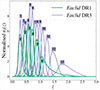 |
Fig. 1. Number density bins simulated for the photometric surveys of Euclid, in 6-bin and 13-bin equi-populated configurations. The numbering convention we used for the ith bin is shown in the coloured blocks above the maxima of each bin. |
3.2.3. DR3 settings
In addition to the initial Euclid data release, we also considered the performance of the flat-sky approximation and Limber approximation for the full data sample of Euclid at the end of the mission. We considered 13 equi-populated bins with a higher (dimmer) magnitude cut at IE < 24.5. The final sample contains a total number density of 24.3 galaxies per arcmin2, and we considered the galaxy and magnification biases measured for this sample in Euclid Collaboration: Mellier et al. (2025). The main specifications are summarised in Table 2 and the galaxy distributions are shown in Fig. 1.
3.3. Assessment of performance
For both survey configurations considered, we wished to assess the accuracy of each of the approximations in recovering the full calculation result, taking into account the uncertainty on the measurement of the power spectra – which, crucially, is largest at small multipoles, and depends on the survey configuration under consideration.
To compare the accuracy of each approximation in the context of real measurements, we simulated noisy power spectra, based on the full CLASS spectra and the theoretical covariance matrix for the planned tomographic bins. In this way, we obtained a set of simulated mock spectra that encompasses the expected spread of measurements, subject to the relevant observational uncertainties (see Tables 2 and 3). Specifically, we took the values of the full spectrum for some subset of multipoles ℓ as the mean, around which we drew 1000 random noise realisations which are normally distributed with a Gaussian covariance (i.e. we neglect non-Gaussian contributions from the connected four-point function). We used the SpaceBorne code2 (Euclid Collaboration: Sciotti et al. 2024) to estimate an analytic Gaussian covariance for the different spectra considered computed using the full spectrum calculation from CLASS. This Gaussian covariance takes the form
![Mathematical equation: $$ \begin{aligned} \mathrm{Cov}\left[C_\ell ^{GG}(i,j)C_{\ell ^{\prime }}^{G^{\prime }G^{\prime }}(k,l)\right] = \frac{1}{2\ell (\ell +1)f_{\rm sky}\varDelta \ell }\delta ^K_{\ell \ell ^{\prime }}&\\ \nonumber \times \left[\left(C_{\ell }^{GG^{\prime }}(i,k)+N_{\ell }^{GG^{\prime }}(i,k)\right)\left(C_{\ell ^{\prime }}^{GG^{\prime }}(j,l)+N_{\ell ^{\prime }}^{GG^{\prime }}(j,l)\right)\right.&\\\nonumber +\left.\left(C_{\ell }^{GG^{\prime }}(i,l)+N_{\ell }^{GG^{\prime }}(i,l)\right)\left(C_{\ell ^{\prime }}^{GG^{\prime }}(j,k)+N_{\ell ^{\prime }}^{GG^{\prime }}(j,k)\right)\right],&\end{aligned} $$](/articles/aa/full_html/2026/03/aa57773-25/aa57773-25-eq38.gif) (23)
(23)
see Equation (138) of Blanchard (2020), where fsky is the fraction of the sky observed, Δℓ is the width of the multipole bins, δℓℓ′K is the Kronecker delta, G indicates the full observed galaxy clustering power spectrum, and indices i, j, k, l run over the tomographic bins. The noise term is given by the shot noise
 (24)
(24)
with  the galaxy surface density per bin in units of inverse steradians.
By comparing to each other the χ2 distributions, formed from the residuals of each method’s result with respect to every one of the spectra in the set of mock observations, we could then obtain an estimate of how far each of the calculations might effectively lie from an observed spectrum, and the frequency with which this occurs.
The χ2 for a particular approximation of the spectra XCℓ, X ∈ {L, F}, with respect to one of the noisy realisations,  , is computed as
 (25)
(25)
where the sum is over values corresponding to 12 bins distributed evenly in the logarithmic space of ℓ, between ℓmin = 2 and ℓmax = 300. In Eq. (26),  is the vector of the residuals,
![Mathematical equation: $$ \begin{aligned} {\boldsymbol{r}}_n^X \mathrm{vech}_{ij}\left[ \hat{C}_n(i,j)-^XC_n(i,j)\right], \end{aligned} $$](/articles/aa/full_html/2026/03/aa57773-25/aa57773-25-eq44.gif) (26)
(26)
with vechij the half-vectorisation operator3, acting on redshift indices of the symmetric tomographic matrix, and  is the inverse of the covariance matrix in a given multipole bin,
  .
.
The covariance (and thus also the mock realisations of the spectra) includes all possible redshift correlations and is calculated for both survey configurations described above. It is often useful to consider the χ2 in the context of the number of degrees of freedom (DOF). In this case, there are N = 12 chosen covariance bins, which effectively act as our ‘data points’, and n redshift bins, leading to n(n + 1)/2 independent spectra of equal and unequal redshift correlations. Thus, we can expect DOFDR1 = N × n × (n + 1)/2 = 252 for DR1 and DOFDR3 = 1092 for DR3.
4. Results
We now present the main results of our analysis. The aim of this section is to quantify the performance of the flat-sky approximation and Limber approximation (for the latter, see also Euclid Collaboration: Cardone et al. 2025; Euclid Collaboration: Joudaki et al. 2025) in the context of Euclid (both for DR1 and DR3 set-ups), assessing how both perform compared to the exact solution.
4.1. Power spectrum recovery
In Figs. 2 and 3 we plot results for the tomographic angular power spectra for the first bin of the DR1 and DR3 configurations, respectively. The true result taken from a full-sky calculation of CLASS is displayed, along with the results using the Limber and flat-sky approximations. The relative error with respect to the full calculation at each multipole is shown in the lower panels.
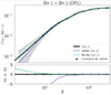 |
Fig. 2. Upper panel: Equal redshift angular power spectrum for the lowest redshift bin of Euclid, using six equi-populated bins. We show the full calculation result from CLASS as a black solid line, and the Limber approximation result as a purple dashed line. The green dashed line corresponds to the recalibrated version of the flat-sky approximation. Lower panel: Relative error (in %) of each approximation from the full calculation result. |
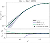 |
Fig. 3. Upper panel: Equal redshift angular power spectrum for the lowest redshift bin of Euclid, using 13 equi-populated bins. We show the full calculation result from CLASS as a black solid line, and the Limber approximation result as a purple dashed line. The green dashed line corresponds to the recalibrated version of the flat-sky approximation. Lower panel: Relative error (in %) of each approximation from the full calculation result. |
We calculated only until ℓ = 300 since, on smaller scales than this, the Limber approximation performs sufficiently well to recover the full calculation result without bias and it is always well within the grey shaded 1σ error band for the survey specifications considered here. We also include an estimate of the error on the observed angular power spectrum, shown as 1σ contours in light grey. In addition, we show an example of the observational effect contributions to the angular power spectrum of DR1 in Fig. 4, for the full calculation from CLASS.
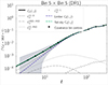 |
Fig. 4. Equal redshift angular power spectrum for the fifth redshift bin of Euclid (DR1). We show the full calculation result from CLASS as a black solid line, and the Limber approximation result as a purple dashed line. The green dashed line corresponds to the recalibrated version of the flat-sky approximation. The various grey lines represent the contributions, from observational effects, to the exact solution (calculated using CLASS). The L-L contribution in this correlation is too insignificant to be visible on these axes. |
Figures 5 and 6, instead, show the relative errors of the approximations for various auto- and cross-bin correlations of the DR3 configuration. In general, the relative errors grow, for unequal redshift correlations between increasingly disparate bins, due to the sensitivity required to detect the smaller signals. In addition, the relative errors do not vary much for equal-z with increasing redshift, though the Limber approximations for the density and redshift terms become worse. This can be understood as a fixed angular scale corresponding to larger co-moving separations as redshift increases, and thus a poorer recovery of the spectrum by the Limber approximation, which completely neglects k∥ – an approximation that becomes worse when k⊥ = ℓ/r(z) gets smaller4. We use this to inform our choice of correlations shown, and in Fig. 5, for the case of DR3, we include correlations in redshift where Limber first becomes significantly different to the full result (Bin 4 × Bin 4), where it reaches one of the most significant departures (Bin 8 × Bin 8), as well as the first bin and last bin equal-z correlations.
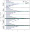 |
Fig. 5. Relative errors in the equal redshift angular power spectrum for redshift bin 1, 4, 8, and 13 of Euclid, using 13 equi-populated bins (DR3). We show the full calculation result from CLASS as a black solid line, and the Limber approximation result as a purple dashed line. The green dashed line corresponds to the recalibrated version of the flat-sky approximation. The relative error associated with the Gaussian covariance calculated at 1σ for the given survey configuration is shown as the grey contour. We note that the y-axis ranges are [ − 50, 50], in contrast to Figs. 2 and 3. |
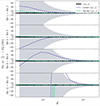 |
Fig. 6. Same as in Fig. 5, but for un-equal redshift bin correlations 1 × 2, 4 × 5, 8 × 9, and 11 × 12 from DR3. The near vertical excursions in the 11 × 12 correlation is due to a zero crossing of the true correlation spectrum. |
Overall, the results from the DR1 configuration show that the improved accuracy of the flat-sky approximation does not result in any useful improvement compared to the Limber approximation in the context of the expected observational error, i.e. it will not be possible to measure the spectra accurately enough to distinguish between the two approximation results. This is true across the entire redshift range, and for correlations between any two redshift bins, though we do not show all these spectra here, for the sake of brevity. This is expected, since the DR1 footprint will be about 10–15% of the full area covered by DR3, meaning that the largest scales, where the discrepancy between Eqs. (7), (9), and (18) is more apparent, will be undersampled with respect to the final data release.
However, in the DR3 configuration, the situation is different. Starting as low as the fourth redshift bin (see second panel from the top in Fig. 5), the Limber approximation fails to recover the spectrum well enough to fall within the 1σ contour. This is also true for the equal-redshift spectra in all of the higher redshift bins, and occurs at relatively low ℓ, where we would expect Limber to encounter difficulty in approximating the spectrum. As in the DR1 case, the Limber approximation of neighbouring bin cross-correlations are not, for the most part, significantly different to the flat-sky approximation results, falling within the 1σ contour for the survey in all but one case (Bin 11 × Bin 12, which is itself merely due to a zero crossing in the full calculation correlation spectrum).
If we consider the individual contributions to the spectra from observational effects, it may provide a hint as to why, in particular, the Limber approximation is insufficient for the full Euclid data release. For the DR1 case (see e.g. Fig. 4), the largest contributions5 are D-D followed by D-L (more important at higher redshift, and correlations between large redshift separated bins). L-L also increases at higher redshift, but is still only of negligible secondary significance with respect to the former two. As expected for a photometric survey, RSDs are not very relevant. RSD-RSD is always smaller than D-D and for each correlation the largest contributions from D-RSD and D-L are of comparable magnitude, with D-RSD being more important at lower ℓ and closer z correlations.
The DR3 case (not shown) is very similar. The major difference is that due to the slimmer redshift bins, the RSD-RSD contribution can be comparable to D-D and D-RSD in the regimes where they are important, i.e. at large scales in correlations of nearby bins (Tanidis & Camera 2019; Euclid Collaboration: Tanidis et al. 2024). The increased overall inaccuracy of the Limber approximation is likely caused by the failure to accurately recover the RSD terms, as a result.
4.2. Simulation results
We then assessed which, if either, of the two approximations is best to model Euclid data, using a χ2 test. This was done by computing the distance between the correct computation of the tomographic harmonic-space power spectra, as per Eq. (7), and the results obtained with either approximation Eqs. (9) and (18). The advantage of this approach is that it takes into account all the possible correlations between different bins, across a range of multipoles ℓ, allowing for the evaluation of the performance as a whole, which is not as easy through simple inspection of the individual spectra alone.
As outlined in Sect. 3.3, we calculated the χ2 distribution of each approximation, given the expected error budget of each survey configuration, arising from 1000 Gaussian realisations of measurement noise. Specifically, we adopted each simulation as a synthetic, noisy data set, and computed the χX2 for both approximations, as per Eq. (26). The further apart these distributions are from the one produced for the CLASS full-sky result, χtrue2, the more sensitive the observations are to differences between the calculated spectra and the full calculation.
We examined the distribution of the true model to verify that the framework of our analysis is returning a reasonable fit to the data, and to give a benchmark for the expected width of the distribution in the case of realistic data. In order to judge whether the model is a good enough description of the data, we can determine the number of degrees of freedom and check whether the mean of the χ2 distribution lies close to this, i.e.  . The overlap in distributions, or Δχ2 > 0, can be associated with a p-value, which acts as a frequentist measure of the probability that each distribution can achieve the χ2 of the full calculation, subject to data uncertainties. Since we ran only 1000 noisy realisations, our smallest possible p-value is 0.001. Our null hypothesis is that the Δχ2 distribution for a particular approximation is consistent with zero. That is, the mean of the χ2 distribution of the approximation is not significantly different to (in this particular case, greater than) that of the full calculation. At the 95% confidence limit, the null hypothesis will be rejected for a p-value less than 0.05, and the distributions can be said not to be consistent at that confidence level. The Δχ2 distribution is particularly useful here, because each sample in the distribution corresponds to the Δχ2 values for corresponding noisy realisations.
In both binning configurations, the full calculation produces a distribution with mean  , indicating that the simulated ‘data’ are reasonable realisations of the true result. In the six equi-populated bin configuration, the mean of the true CLASS distribution is at
  , while for the 13 bin configuration the mean of the true CLASS distribution is at
  .
.
In Fig. 7 we show the distribution for the 1000 values of ΔχX2 ≔ χX2 − χtrue2. For the DR1 case, the result with the Limber approximation includes the dotted zero line, peaking around Δχ2 ∼ 12, whilst the flat-sky approximation only incurs a Δχ2 ∼ 0.2. The p-values for these cases are pLimber = 0.038 and pflat − sky = 0.393, respectively. This means that for the Limber approximation, the null hypothesis is rejected at the 95% confidence level. The flat-sky approximation result is not sufficient to reject the null hypothesis that the Δχ2 distribution is consistent with zero.
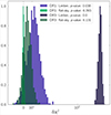 |
Fig. 7. The Δχ2 frequency distributions of the flat-sky (green) and Limber (purple) approximations compared to the full result, with the spread provided by the Gaussian covariance for each survey configuration. The DR1 bin configuration is shown in lighter colours, while the eventual DR3 bin result is shown in darker colours. The improvement of the flat-sky over the Limber approximation is seen in the closer proximity of the former’s distribution to the dotted vertical black line at Δχ2 = 0, most notable in the DR3 bin case. The histograms are each normalised to their own peak values and the x-axis is log-scaled above Δχ2 = 50. |
Comparatively, for the case of the DR3 data, the distinction between the Limber and flat-sky approximations is significantly larger. In terms of the Δχ2, Fig. 7 shows that the flat-sky approximation only reduces the overall recovery of the full calculation result by Δχ2 ∼ 5 on average, with pflat − sky = 0.131, indicating that the null hypothesis that the distribution remains compatible with Δχ2 = 0 still cannot be rejected at 95% confidence. In contrast, the Limber approximation results in a degradation with a distribution which now peaks around Δχ2 ∼ 410, with a p-value at the limit of our number of simulations (pLimber < 0.001), rejecting the null hypothesis at 99%.
5. Discussion
In this paper we compared the performance of the Limber and flat-sky approximations in the determination of the angular power spectra of galaxy number counts from the photometric survey of Euclid. We performed this study in order to assess whether the Limber approximation that enters present standard analysis packages for Euclid, like CLOE (Euclid Collaboration: Cardone et al. 2025; Euclid Collaboration: Joudaki et al. 2025) performs well enough to use for Euclid data. We showed that for the six-bin analysis foreseen with DR1, the Limber approximation is sufficient to model the angular power spectrum. While leading to a slight degradation of χ2 as compared to the full or the flat-sky analysis, it is still able to recover the true result to within the 1σ error, given the survey configuration. This is no longer the case for the DR3, which will be analysed in 13 bins. These bins are sufficiently narrow to render the Limber approximation too crude, with a p-value below 0.1%. In this case the inaccuracies exceed the 1σ errors in the individual equal redshift correlations, resulting in a biased Δχ2 distribution, far-removed from what can reasonably be expected from the covariance in the case of the full calculation. In contrast, the flat-sky approximation is able to maintain accurate recovery of the power spectra, with a p-value of 13.1% at worst, indicating that the overall error introduced by the approximation is small enough to avoid biasing the Δχ2 distribution.
An accurate approximation is only useful if it can also be used to gain computational speed, compared to the full analysis. Since this work does not promote a particular code, we did not conduct an in-depth analysis of the numerical efficiency here. Nevertheless, it is useful to briefly relay the relevant computational timings encountered, to give an idea of the current state of the problem. The 10-fold improvement in performance compared to the full calculation, as reported in Gao et al. (2024), degrades when dealing with wide photometric windows, which require finer meshgrids to achieve accurate results. This involves increasing the number of discretisations in the comoving distance and its derivative, which are controlled by Nchi and Ndchi in the GZCphysics code, and consequently influence the computation time. In order to achieve the level of accuracy described in this work, we found a speed-up of at least two times for ℓ ≳ 130, for our modified version of the flat-sky code with respect to the full calculation. This is still much slower than the Limber approximation, which is, on average, 200 times faster than the full calculation in this case. Furthermore, for ℓ ≲ 100, the current implementation of flat-sky approximation does not save time compared to CLASS. Optimisations to the code in particular are beyond the scope of this work, and left for future analysis.
As the flat-sky calculation still involves a triple integral, a speed up along the lines of the BLAST code (Chiarenza et al. 2024) will be required. However, further optimisations to the flat-sky code are still possible, for example, by optimising the sampling of the radial window functions (Gao et al. 2024). As demonstrated here, the largest deviations of the Limber approximation occur for ℓ ≲ 20 so, in practice, some combination of the two approximations could be used, depending on the relevant scales of the application. Furthermore, for the D-L and L-L contribution, the Limber approximation remains sufficiently accurate, i.e. with deviation less than a few % of cosmic variance from the full numerical result, see Matthewson & Durrer (2021), so that it can certainly be used for well-separated bins where these terms dominate, though the total signal in these bins is small. Indeed, most of the unequal power spectra amplitudes have a contribution that is less than 30% of the corresponding equal redshift amplitude, and never exceeds 50%, which it attains only for the case of neighbouring bin correlation 7 × 8. Finally, the ℓ-dependence of the D-D and RSD-RSD equal redshift terms can be cast as a simple dependence in the lower boundary of the k-integration. Even though the spectrum calculation requires a triple integral, as explained in detail in Gao et al. (2024), the inner k-integration can be pre-computed, which means that the computation time in the case of MCMC parameter estimation would be reduced by of the order of a power of 2/3 for each point in the explored parameter space.
Finally, we address the relevance of this finding for the spectroscopic survey. The spectroscopic number counts are usually analysed by determining the 3D power spectrum which does not employ the Limber approximation. However, a 6 × 2pt analysis, including correlations of the spectroscopic number counts and the shear, is also planned. When using Limber, either one should use wide redshift bins for the spectroscopic survey also, in which case the 6 × 2 analysis does not add anything to the constraints (see Euclid Collaboration: Paganin et al. 2024), or one should choose slim redshift bins. For the redshift bins considered for DR3, we confirm from the results presented in this work that the Limber approximation will be insufficient, and that the flat-sky approximation provides a promising alternative.
Acknowledgments
RD and WM are partially supported by the Swiss National Science Foundation. SC acknowledges support from the Italian Ministry of University and Research (MUR), PRIN 2022 ‘EXSKALIBUR – Euclid-Cross-SKA: Likelihood Inference Building for Universe’s Research’, Grant No. 20222BBYB9, CUP D53D2300252 0006, from the Italian Ministry of Foreign Affairs and International Cooperation (MAECI), Grant No. ZA23GR03, and from the European Union – Next Generation EU. IT has been supported by the Ramon y Cajal fellowship (RYC2023-045531-I) funded by the State Research Agency of the Spanish Ministerio de Ciencia, Innovación y Universidades, MICIU/AEI/10.13039/501100011033/, and Social European Funds plus (FSE+). IT also acknowledges support from the same ministry, via projects PID2019-11317GB, PID2022-141079NB, PID2022-138896NB; the European Research Executive Agency HORIZON-MSCA-2021-SE-01 Research and Innovation programme under the Marie Skłodowska-Curie grant agreement number 101086388 (LACEGAL) and the programme Unidad de Excelencia María de Maeztu, project CEX2020-001058-M. This work has made use of CosmoHub, developed by PIC (maintained by IFAE and CIEMAT) in collaboration with ICE-CSIC. CosmoHub received funding from the Spanish government (MCIN/AEI/10.13039/501100011033), the EU NextGeneration/PRTR (PRTR-C17.I1), and the Generalitat de Catalunya. The Euclid Consortium acknowledges the European Space Agency and a number of agencies and institutes that have supported the development of Euclid, in particular the Agenzia Spaziale Italiana, the Austrian Forschungsförderungsgesellschaft funded through BMK, the Belgian Science Policy, the Canadian Euclid Consortium, the Deutsches Zentrum für Luft- und Raumfahrt, the DTU Space and the Niels Bohr Institute in Denmark, the French Centre National d’Etudes Spatiales, the Fundação para a Ciência e a Tecnologia, the Hungarian Academy of Sciences, the Ministerio de Ciencia, Innovación y Universidades, the National Aeronautics and Space Administration, the National Astronomical Observatory of Japan, the Netherlandse Onderzoekschool Voor Astronomie, the Norwegian Space Agency, the Research Council of Finland, the Romanian Space Agency, the State Secretariat for Education, Research, and Innovation (SERI) at the Swiss Space Office (SSO), and the United Kingdom Space Agency. A complete and detailed list is available on the Euclid web site (www.euclid-ec.org).
References
- Behroozi, P. S., Wechsler, R. H., & Wu, H.-Y. 2013, ApJ, 762, 109 [NASA ADS] [CrossRef] [Google Scholar]
- Blanchard, A., et al. 2020, A&A, 642, A191 [NASA ADS] [CrossRef] [EDP Sciences] [Google Scholar]
- Blanton, M. R., Hogg, D. W., Bahcall, N. A., et al. 2003, ApJ, 592, 819 [Google Scholar]
- Blanton, M. R., Lupton, R. H., Schlegel, D. J., et al. 2005a, ApJ, 631, 208 [Google Scholar]
- Blanton, M. R., Schlegel, D. J., Strauss, M. A., et al. 2005b, AJ, 129, 2562 [NASA ADS] [CrossRef] [Google Scholar]
- Blas, D., Lesgourgues, J., & Tram, T. 2011, JCAP, 7, 034 [Google Scholar]
- Bonvin, C., & Durrer, R. 2011, Phys. Rev. D, 84, 063505 [NASA ADS] [CrossRef] [Google Scholar]
- Carretero, J., Castander, F. J., Gaztañaga, E., Crocce, M., & Fosalba, P. 2015, MNRAS, 447, 646 [NASA ADS] [CrossRef] [Google Scholar]
- Carretero, J., Tallada, P., Casals, J., et al. 2017, in Proceedings of the European Physical Society Conference on High Energy Physics. 5–12 July, 488 [Google Scholar]
- Castorina, E., & White, M. 2018, MNRAS, 479, 741 [NASA ADS] [Google Scholar]
- Challinor, A., & Lewis, A. 2011, Phys. Rev. D, 84, 043516 [NASA ADS] [CrossRef] [Google Scholar]
- Chiarenza, S., Bonici, M., Percival, W., & White, M. 2024, OJAp, 7, 112 [Google Scholar]
- Datta, K. K., Choudhury, T. R., & Bharadwaj, S. 2007, MNRAS, 378, 119 [CrossRef] [Google Scholar]
- Di Dio, E., Montanari, F., Lesgourgues, J., & Durrer, R. 2013, JCAP, 11, 044 [CrossRef] [Google Scholar]
- Di Dio, E., Durrer, R., Marozzi, G., & Montanari, F. 2014, JCAP, 12, 017 [Erratum: JCAP1506, no.06, E01(2015)] [Google Scholar]
- Di Dio, E., Durrer, R., Maartens, R., Montanari, F., & Umeh, O. 2019, JCAP, 04, 053 [Google Scholar]
- Durrer, R. 2020, The Cosmic Microwave Background (Cambridge University Press) [Google Scholar]
- Euclid Collaboration (Blanchard, A., et al.) 2020, A&A, 642, A191 [NASA ADS] [CrossRef] [EDP Sciences] [Google Scholar]
- Euclid Collaboration (Paganin, L., et al.) 2024, A&A, accepted [arXiv:2409.18882] [Google Scholar]
- Euclid Collaboration (Sciotti, D., et al.) 2024, A&A, 691, A318 [NASA ADS] [CrossRef] [EDP Sciences] [Google Scholar]
- Euclid Collaboration (Tanidis, K., et al.) 2024, A&A, 683, A17 [NASA ADS] [CrossRef] [EDP Sciences] [Google Scholar]
- Euclid Collaboration (Cardone, V., et al.) 2025, A&A, submitted [arXiv:2510.09118] [Google Scholar]
- Euclid Collaboration (Castander, F., et al.) 2025, A&A, 697, A5 [Google Scholar]
- Euclid Collaboration (Joudaki, S., et al.) 2025, A&A, submitted [Google Scholar]
- Euclid Collaboration (Mellier, Y., et al.) 2025, A&A, 697, A1 [Google Scholar]
- Euclid Collaboration (Tessore, N., et al.) 2025, A&A, 694, A141 [Google Scholar]
- Fang, X., Krause, E., Eifler, T., & MacCrann, N. 2020, JCAP, 05, 010 [Google Scholar]
- Gao, Z., Raccanelli, A., & Vlah, Z. 2023, Phys. Rev. D, 108, 043503 [Google Scholar]
- Gao, Z., Vlah, Z., & Challinor, A. 2024, JCAP, 02, 003 [Google Scholar]
- Jalilvand, M., Ghosh, B., Majerotto, E., et al. 2020, Phys. Rev. D, 101, 043530 [NASA ADS] [CrossRef] [Google Scholar]
- Kaiser, N. 1992, ApJ, 388, 272 [Google Scholar]
- Kilbinger, M., Heymans, C., Asgari, M., et al. 2017, MNRAS, 472, 2126 [Google Scholar]
- Kitching, T. D., Alsing, J., Heavens, A. F., et al. 2017, MNRAS, 469, 2737 [Google Scholar]
- Leonard, C. D., Ferreira, T., Fang, X., et al. 2023, OJAp, 6, 8 [Google Scholar]
- Limber, D. N. 1954, ApJ, 119, 655 [NASA ADS] [CrossRef] [Google Scholar]
- Martinelli, M., Dalal, R., Majidi, F., et al. 2022, MNRAS, 510, 1964 [Google Scholar]
- Matthewson, W. L., & Durrer, R. 2021, JCAP, 02, 027 [Google Scholar]
- Planck Collaboration VI. 2020, A&A, 641, A6 [Erratum: A&A 652, C4 (2021)] [NASA ADS] [CrossRef] [EDP Sciences] [Google Scholar]
- Potter, D., Stadel, J., & Teyssier, R. 2017, Comput. Astrophys. Cosmol., 4, 2 [NASA ADS] [CrossRef] [Google Scholar]
- Reymond, L., Reeves, A., Zhang, P., & Refregier, A. 2026, JCAP, 2026, 043 [Google Scholar]
- Simon, P. 2007, A&A, 473, 711 [NASA ADS] [CrossRef] [EDP Sciences] [Google Scholar]
- Tallada, P., Carretero, J., Casals, J., et al. 2020, Astron. Comput., 32, 100391 [Google Scholar]
- Tanidis, K., & Camera, S. 2019, MNRAS, 489, 3385 [NASA ADS] [CrossRef] [Google Scholar]
- Tutusaus, I., Martinelli, M., Cardone, V. F., et al. 2020, A&A, 643, A70 [EDP Sciences] [Google Scholar]
- White, M., & Padmanabhan, N. 2017, MNRAS., 471, 1167 [Google Scholar]
- Yoo, J., Fitzpatrick, A. L., & Zaldarriaga, M. 2009, Phys. Rev. D, 80, 083514 [NASA ADS] [CrossRef] [Google Scholar]
- Zehavi, I., Zheng, Z., Weinberg, D. H., et al. 2011, ApJ, 736, 59 [NASA ADS] [CrossRef] [Google Scholar]
- Zuntz, J., Paterno, M., Jennings, E., et al. 2015, Astron. Comput., 12, 45 [NASA ADS] [CrossRef] [Google Scholar]
The vectorisation of a matrix converts a matrix into a vector, for example by stacking columns on top of each other. In the case of a symmetric matrix of size n × n, only the n (n + 1)/2 independent entries are stacked.
At larger scales, where naïve geometric intuition seems to suggest that the flat-sky approximation should also fail, it is actually impressively accurate. This has been noted before Matthewson & Durrer (2021).
We use the shorthand D for density, RSD for redshift space distortions, and L for lensing. Here we are referring to cross-correlations between these terms. For example, ‘D-D’ refers to the density-density contribution to the angular power spectrum of galaxy number counts.
All Tables
Cosmological parameters for the Flagship simulation (from the Euclid reference cosmology), and the fiducial cosmology used in the current work, from Planck 2018 (‘TT, TE, EE+lowE+lensing+BAO’ results, Planck Collaboration VI 2020).
Summary of survey specifications used in SpaceBorne to calculate the covariance of each binning configuration (Euclid Collaboration: Mellier et al. 2025).
Linear galaxy bias factor, b(z), and magnification bias, s(z, L), for the six-bin configuration of Euclid.
All Figures
|
Fig. 1. Number density bins simulated for the photometric surveys of Euclid, in 6-bin and 13-bin equi-populated configurations. The numbering convention we used for the ith bin is shown in the coloured blocks above the maxima of each bin. |
| In the text | |
|
Fig. 2. Upper panel: Equal redshift angular power spectrum for the lowest redshift bin of Euclid, using six equi-populated bins. We show the full calculation result from CLASS as a black solid line, and the Limber approximation result as a purple dashed line. The green dashed line corresponds to the recalibrated version of the flat-sky approximation. Lower panel: Relative error (in %) of each approximation from the full calculation result. |
| In the text | |
|
Fig. 3. Upper panel: Equal redshift angular power spectrum for the lowest redshift bin of Euclid, using 13 equi-populated bins. We show the full calculation result from CLASS as a black solid line, and the Limber approximation result as a purple dashed line. The green dashed line corresponds to the recalibrated version of the flat-sky approximation. Lower panel: Relative error (in %) of each approximation from the full calculation result. |
| In the text | |
|
Fig. 4. Equal redshift angular power spectrum for the fifth redshift bin of Euclid (DR1). We show the full calculation result from CLASS as a black solid line, and the Limber approximation result as a purple dashed line. The green dashed line corresponds to the recalibrated version of the flat-sky approximation. The various grey lines represent the contributions, from observational effects, to the exact solution (calculated using CLASS). The L-L contribution in this correlation is too insignificant to be visible on these axes. |
| In the text | |
|
Fig. 5. Relative errors in the equal redshift angular power spectrum for redshift bin 1, 4, 8, and 13 of Euclid, using 13 equi-populated bins (DR3). We show the full calculation result from CLASS as a black solid line, and the Limber approximation result as a purple dashed line. The green dashed line corresponds to the recalibrated version of the flat-sky approximation. The relative error associated with the Gaussian covariance calculated at 1σ for the given survey configuration is shown as the grey contour. We note that the y-axis ranges are [ − 50, 50], in contrast to Figs. 2 and 3. |
| In the text | |
|
Fig. 6. Same as in Fig. 5, but for un-equal redshift bin correlations 1 × 2, 4 × 5, 8 × 9, and 11 × 12 from DR3. The near vertical excursions in the 11 × 12 correlation is due to a zero crossing of the true correlation spectrum. |
| In the text | |
|
Fig. 7. The Δχ2 frequency distributions of the flat-sky (green) and Limber (purple) approximations compared to the full result, with the spread provided by the Gaussian covariance for each survey configuration. The DR1 bin configuration is shown in lighter colours, while the eventual DR3 bin result is shown in darker colours. The improvement of the flat-sky over the Limber approximation is seen in the closer proximity of the former’s distribution to the dotted vertical black line at Δχ2 = 0, most notable in the DR3 bin case. The histograms are each normalised to their own peak values and the x-axis is log-scaled above Δχ2 = 50. |
| In the text | |
Current usage metrics show cumulative count of Article Views (full-text article views including HTML views, PDF and ePub downloads, according to the available data) and Abstracts Views on Vision4Press platform.
Data correspond to usage on the plateform after 2015. The current usage metrics is available 48-96 hours after online publication and is updated daily on week days.
Initial download of the metrics may take a while.