| Issue |
A&A
Volume 707, March 2026
|
|
|---|---|---|
| Article Number | A27 | |
| Number of page(s) | 14 | |
| Section | Astrophysical processes | |
| DOI | https://doi.org/10.1051/0004-6361/202557948 | |
| Published online | 25 February 2026 | |
Radiative cooling effects on plasmoid formation in black hole accretion flows with multiple magnetic loops
1
Tsung-Dao Lee Institute, Shanghai Jiao Tong University 1 Lisuo Road Shanghai 201210, PR China
2
School of Physics and Astronomy, Shanghai Jiao Tong University 800 Dongchuan Road Shanghai 200240, PR China
3
Key Laboratory for Particle Physics, Astrophysics and Cosmology (MOE), Shanghai Key Laboratory for Particle Physics and Cosmology, Shanghai Jiao Tong University 800 Dongchuan Road Shanghai 200240, PR China
4
Institut für Theoretische Physik, Goethe-Universität Frankfurt Max-von-Laue-Str 1 D-60438 Frankfurt am Main, Germany
5
Research Center for Astronomy, Academy of Athens Soranou Efessiou 4 GR-11527 Athens, Greece
6
Institut für Theoretische Physik und Astrophysik, Universität Würzburg Emil-Fischer-Str. 31 D-97074 Würzburg, Germany
7
Max-Planck-Institut für Radioastronomie Auf dem Hügel 69 D-53121 Bonn, Germany
★ Corresponding authors: This email address is being protected from spambots. You need JavaScript enabled to view it.
; This email address is being protected from spambots. You need JavaScript enabled to view it.
; This email address is being protected from spambots. You need JavaScript enabled to view it.
Received:
3
November
2025
Accepted:
16
January
2026
Abstract
Context. We investigated the physics of black hole accretion flows, particularly focusing on phenomena like magnetic reconnection and plasmoid formation, which are believed to be responsible for energetic events such as flares observed from astrophysical black holes.
Aims. We aim to understand the influence of radiative cooling on plasmoid formation within black hole accretion flows that are threaded by multi-loop magnetic field configurations.
Methods. We conducted 2D and 3D two-temperature general relativistic magnetohydrodynamic simulations. By varying the magnetic loop sizes and the mass accretion rate, we explored how radiative cooling alters the accretion dynamics, disk structure, and properties of reconnection-driven plasmoid chains.
Results. Our results demonstrate that radiative cooling suppresses the transition to the magnetically arrested disk state by reducing magnetic flux accumulation near the horizon. It significantly modifies the disk morphology by lowering the electron temperature and compressing the disk, which leads to increased density at the equatorial plane and decreased magnetization. Within the current sheets, radiative cooling triggers layer compression and the collapse of plasmoids, shortening their lifetime and reducing their size, while the frequency of plasmoid events increases. Moreover, we observe enhanced negative energy-at-infinity density in plasmoids near the ergosphere, with its peaks corresponding to plasmoid formation events.
Conclusions. Radiative cooling plays a critical role in shaping both macroscopic accretion flow properties and microscopic reconnection phenomena near black holes. This suggests that radiative cooling modulates black hole energy extraction through reconnection-driven Penrose processes, highlighting its importance in models of astrophysical black holes.
Key words: black hole physics / magnetic fields / magnetic reconnection / magnetohydrodynamics (MHD) / relativistic processes
© The Authors 2026
 Open Access article, published by EDP Sciences, under the terms of the Creative Commons Attribution License (https://creativecommons.org/licenses/by/4.0), which permits unrestricted use, distribution, and reproduction in any medium, provided the original work is properly cited.
This article is published in open access under the Subscribe to Open model. This email address is being protected from spambots. You need JavaScript enabled to view it. to support open access publication.
1. Introduction
Over the past few decades, the black hole (BH) candidate at the center of the Milky Way, Sagittarius A* (hereafter Sgr A*), has served as an exceptional laboratory for studying the physics of accretion and outflows due to its proximity to Earth. Numerous in-depth observational and theoretical studies on the morphology, variability, and other characteristics of Sgr A* have been conducted (Markoff & Event Horizon Telescope Collaboration 2022; Event Horizon Telescope Collaboration 2022a; Ripperda et al. 2022). Episodic flares are detected across the electromagnetic spectrum, attracting great interest from the astronomical community.
Despite extensive efforts, the precise mechanism responsible for these flares remains a matter of debate. Several mechanisms have been proposed, including flux eruption events (Porth et al. 2021; Antonopoulou et al. 2025), magnetic reconnection (Lin & Yuan 2024; Lin et al. 2023), and plasmoid chains along the current sheet (Dimitropoulos et al. 2025). These processes collectively contribute to the observed variability and energetic phenomena near the BH (Trippe et al. 2007; Yuan et al. 2004). Observations by the Event Horizon Telescope (EHT) of Sgr A* suggest the presence of a strong and ordered magnetic field (Event Horizon Telescope Collaboration 2024). These results indicate a preference for the magnetically arrested disk (MAD) regime over the standard and normal evolution (SANE) regime and other types of accretion flows (Event Horizon Telescope Collaboration 2022a, 2024, 2022b). However, powerful jets are typically associated with the MAD accretion regime (Chavez et al. 2024; Narayan et al. 2022), and there have been no observations of such a jet in observations, suggesting that our current models are incomplete.
Large-scale magnetized jets generated by accretion flows around BHs often exhibit variable energy output (Nathanail et al. 2020). Due to the inherently turbulent nature of the accretion process (Liska et al. 2022), magnetic field loops of differentpolarities are generated around the BH. The merging of the magnetic loops causes frequent polarity inversion events and forms current sheets (Ripperda et al. 2022; El Mellah et al. 2023; Kumar et al. 2015). The tearing instability in the current sheets creates plasmoids and x-points, making them ideal places for particle acceleration and the flaring events of Sgr A* via magnetic reconnection (Tchekhovskoy et al. 2009; Ripperda et al. 2017, 2019; GRAVITY Collaboration 2018, 2023; Ripperda et al. 2022).
High-resolution general relativistic magnetohydrodynamic (GRMHD) simulations show that mean-field dynamo and magnetorotational instability can transform toroidal magnetic fields into poloidal loops, creating a multi-loop magnetic configuration in accretion tori (Liska et al. 2020; Kaufman et al. 2023; Gottlieb et al. 2023; Rodman & Reynolds 2024). To mimic this process, simulations with initial multi-loop magnetic field configurations have been performed to study the dynamics of the accretion flows (Nathanail et al. 2020, 2022; Jiang et al. 2023, 2024). The alternating polarity configuration not only prevents the accumulation of magnetic fields but also facilitates frequent reconnection between magnetic loops of opposite polarities, thereby releasing magnetic energy. A series of 2D GRMHD simulations with multi-loop configurations was conducted by Nathanail et al. (2020), and 3D simulations with multi-loop magnetic field configurations were performed by Chashkina et al. (2021) and Nathanail et al. (2022). These studies demonstrate that the multi-loop magnetic field configuration can efficiently produce energetic plasmoids via magnetic reconnection, which have been proposed to explain flaring events from Sgr A* (Petropoulou et al. 2016; Zhang et al. 2018; Christie et al. 2019). Another possible explanation for these flares is the energy release during flux eruption events in the MAD state, which also provide suitable conditions for accelerating nonthermal particles (Jiang et al. 2025; Chashkina et al. 2021; Scepi et al. 2022; Jiang et al. 2023; Grigorian & Dexter 2024). Unlike SANE models, which typically produce only weak jets, MAD models generally yield powerful jets. However, there is no clear, strong observational evidence of such a powerful jet in Sgr A* (Event Horizon Telescope Collaboration 2022a).
Recent studies suggest that radiative cooling can reduce jet efficiency by a factor of approximately 2 (Singh et al. 2025), making the MAD configuration with radiative cooling a more plausible explanation for Sgr A*. The bolometric luminosity of Sgr A* is extremely low, Lbol ∼ 1036 erg s−1 ≈ 10−9LEdd, where LEdd represents the Eddington luminosity (Event Horizon Telescope Collaboration 2022a). Given this extremely low luminosity, radiative cooling has conventionally been regarded as negligible, as it is unlikely to substantially affect the dynamics of the accretion flow. Most previous studies employing 3D GRMHD simulations have omitted radiative cooling losses for simplicity (Ryan et al. 2018; Jiang et al. 2023, 2024). While this assumption is generally reasonable, Dibi et al. (2012) argued, based on their 2D simulations, that cooling losses become increasingly important at higher accretion rates, i.e., Ṁ ≳ 10−7 ṀEdd. Similar results were also obtained by Dihingia et al. (2023). These losses may influence the dynamics and spectra of Sgr A*, even within the permitted range of accretion rates inferred from polarization and X-ray studies (Chael 2025; Salas et al. 2025). It is worth noting that single-fluid GRMHD simulations that incorporate radiative cooling have also been employed to investigate hot accretion flows around Sgr A* (Fragile & Meier 2009; Dibi et al. 2012; Drappeau et al. 2013; Yoon et al. 2020). The influence of radiative cooling on accretion flow dynamics intensifies with the accretion rate. Specifically, when the accretion rate exceeds approximately 10−7 ṀEdd, radiative cooling plays an increasingly significant role in shaping the dynamical properties of the accretion disk (Yoon et al. 2020) and their horizon-scale images.
With the advancement of astronomical observations and numerical simulations, BHs have emerged as unique laboratories for testing plasma electrodynamics under extreme conditions (Lasota et al. 2014). Among the most profound predictions of general relativity is the possibility of extracting rotational energy from a BH via the inflow of negative energy and angular momentum across the event horizon (Penrose & Floyd 1971). Recently, the nonlinear nature of magnetic reconnection and plasma dynamics near the surface of the accretion tori around BHs has been increasingly recognized (Asenjo & Comisso 2015), and it has been reported that energy extraction can occur during the formation of plasmoid chains via the Penrose process (PP; Fan et al. 2024; Shen & YuChih 2025). Most past studies on this subject have been conducted within purely analytical frameworks. In this work, we extend the investigation by performing numerical simulations and analysis within a multi-loop configuration that incorporates the effects of radiative cooling.
We performed a series of 2D two-temperature GRMHD simulations with a multi-loop initial magnetic field configuration to investigate the effect of radiative cooling. Specifically, we studied the influence of radiative cooling on plasmoid chains, conducting statistical analysis on their properties, including radii and occurrence rates. To confirm the generality of the conclusions obtained from 2D simulations, we also performed 3D GRMHD simulations and high-resolution 2D GRMHD simulations to further study the disk and temperature properties caused by radiative cooling.
This paper is organized as follows. In Sect. 2 we describe the simulation setup. In Sect. 3 we report our main results on the effects of radiative cooling. Finally, Sect. 4 summarizes our main findings and provides a discussion.
2. Numerical setup
Our GRMHD simulations were conducted with the BHAC code (Porth et al. 2017; Olivares et al. 2019). BHAC code solves the ideal magnetohydrodynamic equations in geometric units (G = M = c = 1), which are given in equations expressed in covariant notation as follows:
 (1)
(1)
which express the conservation of mass, the energy-momentum tensor (Tμν), and the homogeneous Maxwell equations, respectively. The Faraday tensor (Fμν) further characterizes the electromagnetic fields in the system. In GRMHD codes, Eq. (1) is transformed into conservative form through the 3+1 formalism, which is written as (Del Zanna et al. 2007; Porth et al. 2017)
 (2)
(2)
where the specific formulation of terms U, F and S are the conserved variables, fluxes and source term. Following Dihingia et al. (2023), we incorporated radiative cooling by implementing the modified source term S = S0 + S′, where S′ accounts for contributions from radiative cooling processes, as detailed in Dihingia et al. (2023). The explicit form of the additional source term S′ is expressed as
 (3)
(3)
where α is the lapse function, γ is the Lorentz factor, vj represents the fluid three-velocity, and Λ is the total radiative cooling term, which includes synchrotron cooling and bremsstrahlung cooling. The explicit form of dissipative heating, Coulomb interaction, and radiative cooling processes are introduced in Sect. 2.2.
2.1. Model setup
The simulations are initialized with Fishbone-Moncrief hydrodynamic equilibrium torus (Fishbone & Moncrief 1976), with parameters rin = 20 rg and rmax = 40 rg, where rg ≡ GM/c2 is the gravitational radius, G is gravitational constant and M is the BH mass. An ideal gas equation of state is adopted, with a constant adiabatic index of Γ = 4/3.
In all cases, we considered a purely poloidal magnetic field as an initial condition. The initial magnetic configuration is given by defining the vector potential as follows:
 (4)
(4)
To control the number of magnetic loops in the vertical and radial directions, the vector potential Aϕ is further multiplied by cos((N − 1)θ) and sin(2π(r−rin)/λr), where λr represents the radial loop wavelength, and N is the number of magnetic loops in the θ-direction. For all cases, following Jiang et al. (2023), we set N = 3.
Our simulations use spherical modified Kerr–Schild coordinates. The simulation domain extends radially from the BH event horizon to r = 2500 rg with a logarithmic spacing. In the polar direction, the domain spans from the polar angle θ = 0 to π with uniform spacing. In all 2D simulations, we adopted a standard resolution of 1024 × 512, except for one high-resolution case with an effective resolution of 4096 × 2048 (see Appendix B for details on the numerical setup). For the 3D simulations, we employed two levels of static mesh refinement, achieving an effective resolution of 320 × 160 × 160. The 2D simulations were evolved until t = 15000 M, while the 3D simulations were extended to t = 25000 M to reach quasi-steady state.
To excite the magnetorotational instability, we applied a 2% random perturbation to the gas pressure within the torus. We adopted a floor treatment to ensure numerical stability in low-density regions, particularly near the BH and the rotation axis (Giulini 2015). Specifically, the floor values for the rest-mass density and pressure were set to ρfl = 10−4r−3/2 and pfl = (10−6/3)r−5/2, respectively. For the electron pressure, we used pe = 0.01pfl for pe ≤ 0.01pfl and pe = 0.99pg for pe ≥ 0.99pg, where pg is the gas pressure. Additionally, the entropy of the gas (κg) and the electrons (κe) are recalculated, where the floor condition is applied. In all simulations, the BH mass and spin are set to MBH = 4.5 × 10⁶ M⊙ and a* = 0.9375, respectively.
To conduct a comprehensive investigation of various scenarios, we considered several simulation models. The details of these models are summarized in Table 1.
Model parameters: λr, the mass accretion rate normalized by the Eddington ratio, the radiative cooling status, and the grid number.
2.2. Radiative cooling
Following Ressler et al. (2015) and Sądowski et al. (2017), we solved the electron-entropy equation in the presence of dissipative heating, Coulomb interaction, and radiative cooling processes:
 (5)
(5)
where κe := exp[(Γe − 1)se] and se := p/ρΓe represent the electron entropy per particle. Here, Γe denotes the adiabatic index of the electrons; we used Γe = 4/3, Q is the rate of dissipative heating, and fe is the fraction of dissipative heating transferred to the electrons. Λei is the energy transferred to the electrons from the ions through Coulomb interaction, and Λ represents the radiative cooling term. The radiative cooling rate is computed following Dibi et al. (2012) and Dihingia et al. (2023), using the solutions from Esin et al. (1996) to account for bremsstrahlung, synchrotron, and inverse Compton cooling processes (see Appendix A for detailed calculations). Solving the fluid equations (Eq. (1)) together with the electron-entropy equation (Eq. (5)) yields all relevant properties of the accretion flows and electron thermodynamics.
3. Influence of radiative cooling on accretion flows
3.1. Comparison of properties in the accretion flow
This section investigates the impact of radiative cooling on the accretion process by analyzing the mass accretion rate (Ṁ) and magnetic flux (ΦB) through the BH horizon. Our 2D simulations include six different runs with different initial magnetic field configurations and radiative cooling setup. Following Porth et al. (2019), we defined the mass accretion rate Ṁ and magnetic flux ΦBH near the BH horizon as follows:
 (6)
(6)
 (7)
(7)
where ρ is the rest-mass density, ur is the radial component of the four-velocity, Br is the radial magnetic field, and  is the square root of the metric determinant.
In Fig. 1, the time evolutions of mass accretion rate Ṁ and normalized magnetic flux  of the models are presented. Panels (a) and (c) of Fig. 1 depict models initialized with smaller magnetic loops (wavelength λr = 40), while panels (b) and (d) show models with larger magnetic loops (wavelength λr = 80). Different colors in these panels indicate variations in the values of mass accretion rate normalized by Eddington ratio, ṀEdd, and with or without radiative cooling. The dashed lines in the panels represent
  , which is the criterion for MAD regime (Tchekhovskoy et al. 2011; Mizuno et al. 2021).
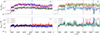 |
Fig. 1. Time evolution of mass accretion rates measured at the event horizon (top) and the normalized magnetic flux at the horizon (bottom). Panels (a) and (c): Case with smaller magnetic loops (λ = 40). Panels (b) and (d): Case with larger magnetic loops (λ = 80). The curves in different colors correspond to the different radiative cooling and time-averaged accretion rates: radiative cooling with Ṁ/ṀEdd = 1 × 10⁻³ (blue and green), radiative cooling with 1 × 10⁻⁵(black and light blue), and no cooling (red and light red). In panel (c), the horizontal red and blue lines denote the average magnetic flux of models A and C, respectively. The blue vertical lines in panels (a) and (c) mark the onset of the quasi-steady state. In panels (b) and (d), the light blue and light red vertical lines indicate the transition from SANE to MAD for models E and F, respectively. The time is given in units of the light crossing time, tg ≡ GM/c3 = [M]. |
From the magnetic flux evolutions in Fig. 1, we observe a decreased magnetic flux from the models with stronger cooling. The vertical blue lines in the panel indicates the moment the accretion flow achieves a quasi-steady state for smaller magnetic loop cases. The horizontal lines represent the average normalized magnetic flux during this period. In the quasi-steady state, the non-cooling case (red line) exhibits greater magnetic flux accumulation compared to the case with radiative cooling (blue line). Due to the relatively small magnetic loops, the accretion flows do not reach the MAD regime (Jiang et al. 2023). Radiative cooling mostly reduces the magnetic flux, which is also evident in models D, E, and F in the larger loop runs in Fig. 1d. We note, however, that the cooling-induced reduction of the normalized magnetic flux at the event horizon may not be universal. Recent work by Singh et al. (2025) demonstrated that the response of the MAD parameter to radiative cooling can depend sensitively on the BH spin, with different spin values exhibiting distinct trends in magnetic flux accumulation. In the present study, we restricted our analysis to a single BH spin configuration and therefore did not explore this additional parameter space. We focused on a rapidly spinning BH with a = 0.9375, motivated by observational constraints suggesting that Sgr A* likely possesses a high spin (Event Horizon Telescope Collaboration 2022b). Consequently, while our results indicate a systematic suppression of magnetic flux with increasing cooling strength for the spin considered here, a broader survey over BH spins will be required to establish the generality of this behavior.
For the larger loop models (wavelength λr = 80 rg), shown in the right panels of Fig. 1, fewer magnetic loops within the torus result in reduced magnetic dissipation between them. The merging of these loops generates abundant small-scale magnetic fields, which initially prevent significant magnetic field accumulation near the BH, producing a SANE-type flow in the early stages of the simulations. As these small-scale fields coalesce into a more ordered, large-scale magnetic structure, the accretion flow transitions from a SANE to a MAD regime, as observed in Fig. 1d after the vertical lines. The light blue and light red vertical lines indicate the transition time from SANE to MAD regime. From model E (light blue lines), which has a relatively weak cooling effect, we see a delayed transition to the MAD regime compared to the non-cooling case (model F, light red lines). While in model D (green lines), the cooling effect is so strong that the SANE to MAD transition does not occur within the simulation duration. Radiative cooling reduces the accumulation of magnetic flux near the BH horizon, resulting in insufficient magnetic flux pile-up to reach the MAD regime.
Similar behavior is also seen in the 3D simulations in Fig. 2. Radiative cooling suppresses the accumulation of magnetic flux, consistent with the conclusions drawn from our 2D simulations.
3.2. The influence of radiative cooling
3.2.1. Electron temperature
The most direct impact of radiative cooling on our simulations is the substantial alteration of electron temperature. To illustrate the effects of radiative cooling on the physical structure of the disk, in Fig. 3, we show the time-averaged profiles of the electron temperature (Θe), plasma beta (β), and density (ρ) for models A, B, and C. These quantities are averaged over the time interval t = 8000–13 000 M, during which the mass accretion rate remains approximately steady. We used the two-temperature approach to calculate the time evolution of electron entropy following (Ressler et al. 2015; Mizuno et al. 2021). The energy injection ratio to electron and ion comes from the prescription based on turbulent plasma in Kawazura et al. (2019); see more details in Mizuno et al. (2021) and Jiang et al. (2023). The electron pressure (pe) was calculated as  , where the value of κe was updated according to Eq. (3) in Mizuno et al. (2021). The ion-to-electron temperature ratio is then determined as Ti/Te = (pg−pe)/pe. The dimensionless electron temperature (Θe) is defined as
 (8)
(8)
where pg is the total gas pressure, ρ is the density, mp and me are the proton and electron masses, respectively, and Ti and Te are the ion and electron temperatures.
In the left column of Fig. 3, the electron temperature of the simulations with different magnitudes of cooling are presented. We confirm that radiative cooling reduces the overall electron temperature, particularly in the disk region. The extent of this reduction depends on the cooling intensity, consistent with the findings of Dihingia et al. (2023). However, radiative cooling not only globally decreases the electron temperature but also further impacts the associated dynamics and structure of the accretion disk. Due to the radiative loss of thermal energy, the gas pressure is reduced, leading to a lower scale height of the disk. In the right column of Fig. 3, we present the average density distributions of models A, B, and C. It is evident that the temperature reduction induced by radiative cooling significantly increases the density in the disk, resulting in vertical compression in disk height. To quantify the geometric structure of the disk, we computed the density-weighted scale height (H), following the definition in Noble et al. (2009):
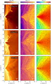 |
Fig. 3. Time-averaged electron temperature (Θe), plasma β, and density (ρ) distributions for models A, B, and C (from top to bottom). The plasma beta parameter is defined as β = pg/pmag, where pg represents the gas pressure, and pmag = b2/2 denotes the magnetic pressure. The black contours in the density profile represent the magnetic field. The average is taken over the time range t = 8000 M to 13 000 M. |
where z = r cos θ, and the angle brackets ⟨ ⋅ ⟩ denote density-weighted shell averages:
Here, σ < 1 denotes the integration domain within the disk region. As shown in Fig. 4, radiative cooling leads to a clear reduction in the disk scale height, particularly in the inner regions. This flattening of the disk reflects the loss of internal energy and thermal pressure support due to radiative losses. For models with stronger radiative cooling, the increase in density compared to the no-cooling model is more pronounced and extends over a wider radial extent. Furthermore, the middle column of Fig. 3 illustrates that radiative cooling leads to the formation of a more ordered and high-beta region, which in turn suppresses the effectiveness of the magnetorotational instability in shaping the disk structure and contributes to a thinner disk.
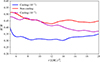 |
Fig. 4. Density-weighted scale height as a function of radius for cooling models A, B, and C. |
Figure 5 presents azimuthal- and time-averaged polar-angle profiles of the ion-to-electron temperature ratio of different cooling models at r = 15 M. We observe that both model A (with cooling) and model C (without cooling) exhibit a higher ion-to-electron temperature ratio near the equatorial plane compared to other polar angles; similar plots have been shown by Mizuno et al. (2021). Model A tends to exhibit a globally higher ion-to-electron temperature ratio compared to both the no-cooling case (model C) and the weaker cooling case (model B). It is worth noting that in both model B and model C, the ion temperature remains lower than the electron temperature (Ti < Te) throughout the domain. In contrast, model A exhibits a region near the equatorial plane where Ti > Te, due to the radiative cooling, which primarily reduces the electron temperature in the disk region. While model A still shows Ti < Te toward the polar regions, consistent with the other models. This behavior arises because most of the electron heating occurs around the funnel region. Consistent with our expectations, the high-resolution simulations reproduce similar trends observed in the low-resolution runs, confirming the influence of radiative cooling on the thermodynamic structure of the accretion flows.
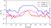 |
Fig. 5. Azimuthal and time-averaged polar-angle profiles of the ion-to-electron temperature ratio of models A, B, and C at r = 15 M. The averaging time range is the same as used in Fig. 3. |
In our 3D simulations, the disk exhibits similar features under the influence of radiative cooling. As shown in Fig. 6, radiative cooling leads to a noticeable vertical compression of the disk, which in turn results in an increase in the density. Interestingly, in model M40a3d shown in Fig. 6, we clearly observe that radiative cooling leads to a lower density in the funnel region. Radiative cooling also causes more matter to accumulate near the equatorial plane, resulting in a cleaner (i.e., lower-density) environment away from the midplane. Moreover, reducing gas pressure in the disk suppresses the radial transport of mass and magnetic flux to the BH. Because the magnetic flux threading the BH is reduced, it is limiting the power available for the Blandford–Znajek mechanism. Thus, jet efficiency becomes decreased with radiative cooling (Singh et al. 2025).
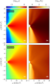 |
Fig. 6. Distribution of the time-averaged density and electron temperature at ϕ = 0 for the models (with cooling and without cooling) in the averaging range t = 10000 M–14000 M. |
Consistent with the findings in the 2D simulations of Jiang et al. (2023), we observe that a smaller magnetic loop configuration can lead to the emergence of a one-sided jet. The same conclusions are obtained across simulations with different dimensionality.
As discussed in Sect. 3.1, radiative cooling also reduces the accumulation of poloidal magnetic flux. This effect is likewise captured in the cross-sectional slices of our 3D simulations as shown in Fig. 7. A more detailed discussion of this phenomenon is provided in Sect. 3.2.4.
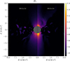 |
Fig. 7. Distribution of the axial component of the magnetic field (Bz) in a cross-sectional slice at t = 7920 M for models M40a3d (left) and M40n3d (right). |
3.2.2. Radiative collapse and plasmoid formation
Besides of the global effects of radiative cooling on the accretion flow properties, it also significantly affects small-scale structures. When radiative cooling is included, the reconnection layer exhibits noticeable instabilities. Plasmoids formed via tearing instability tend to collapse due to enhanced cooling effects. This process, known as radiative collapse, occurs when cooling-driven compression further amplifies the cooling rate, leading to a so-called runaway collapse of the current sheet (Dorman & Kulsrud 1995; Uzdensky & McKinney 2011). As radiative losses deplete the internal energy within the reconnection layer, the temperature of the layer decreases. To maintain pressure equilibrium in the region, the density within the layer correspondingly increases to offset the lower temperature. This compression, in turn, increases the radiation, resulting in a feedback loop of runaway compression and cooling of the layer.
The relationship between plasmoid formation and plasma instabilities has been explored in previous studies (e.g., Loureiro et al. 2012; Ni et al. 2017). The Kelvin-Helmholtz instability is one mechanism that facilitates plasmoid formation at the shear boundary between the jet funnel and sheath regions. The tearing instability, on the other hand, is commonly associated with magnetic reconnection through an extended thin current sheet, resulting in plasmoid chains. Ripperda et al. (2022) examined the development of plasmoid chains in the equatorial plane under the MAD state. Similar plasmoid chain formation is observed in our simulations. In this study, we investigated the properties of these plasmoids in greater detail.
As radiative losses deplete internal energy from the reconnection layer, its temperature decreases. In response, the density increases to maintain pressure equilibrium, as previously discussed, ultimately leading to collapse. In addition to radiative collapse, the reconnection layer may also be subject to local radiative cooling instabilities (Field 1965). These instabilities arise from pressure perturbations that become unstable under radiative cooling. The interaction between these thermal and the tearing instabilities can play a significant role in shaping the transient dynamics of the reconnection process (Forbes & Malherbe 1991). In our simulations, we observe a collapse induced by radiative cooling.
As shown in upper panels of Fig. 8, we focused on the evolution of a single plasmoid chain in high-resolution strong cooling model hr, which effectively illustrates the process of radiative collapse under radiative cooling. As predicted, the plasmoids in the chain become cooler (dimmer) as they evolve outward, ultimately collapsing under strong compression. Additionally, we checked the density distribution around the plasmoid chain shown in the lower panel in Fig. 8. The temporal evolution of integrated electron temperature and density in the vicinity of plasmoids is shown in Fig. 9. It is evident that, as the plasmoid chain evolves, the surrounding electron temperature decreases while density gradually increases, explaining why the plasmoids eventually undergo radiative collapse. Similar phenomena are also observed in the lower-resolution simulations, as shown in Fig. B.2.
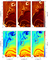 |
Fig. 8. Time evolution of a plasmoid chain in the high-resolution model hr over the time interval t = 8170 M to t = 8180 M. Upper panel: Electron temperature. Lower panel: Density. We mark the location of the plasmoid chain with a red box in each panel. |
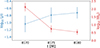 |
Fig. 9. Time evolution of the integrated density (blue) and electron temperature (red) of a tracked plasmoid in the interval shown in Fig. 8. |
3.2.3. Statistical properties of plasmoids
In order to analyze the statistical properties of plasmoids with radiative cooling, we aimed to detect them in the simulations. We applied a plasmoid detection method based on Nathanail et al. (2020), by tracking blob-like structures in our simulations using the scikit-image package (Van der Walt et al. 2014). This approach allows us to capture the positions and sizes of the plasmoids within a selected region, which extends from 0 to 20 rg in x-direction and from −20 to 20 rg in y-direction of the snapshots with a cadence of 10 M. We applied the same detection criteria to all models to ensure generalizability. We also constrained the regions where the Bernoulli constant (−hut) is greater than 1.02 for this plasmoid detection.
As discussed in Sect. 3.2.2, radiative cooling leads to the collapse of the plasmoids. This implies that the number of detected plasmoids decreases after the collapse occurs. In Fig. 10, we plot the time evolution of number of plasmoids in different models. In the presence of radiative cooling, radiative collapse causes the plasmoid to dissipate and gradually vanish. Compared to cases without radiative cooling, this collapse shortens the lifetime of the plasmoid chain. This results in a spikier structure in the plasmoid count evolution.
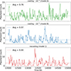 |
Fig. 10. Time evolution of the number of detected plasmoids in different models: cooling with Ṁ/ṀEdd = 10−3(top), cooling with Ṁ/ṀEdd = 10−5 (middle), and non-cooling (bottom). |
In our ideal GRMHD framework (i.e., physical resistivity η = 0), all resistive effects arise from numerical dissipation. From our second-order numerical accuracy of the BHAC code (Porth et al. 2017), the effective numerical resistivity scales as ηnum ∼ Δxp with p ≈ 2. As a result, the Lundquist number, defined as SL = VAL/η, remains independent of local temperature variations.Here, VA and L denote the Alfvén speed and the size of the reconnection layer, respectively. The normalized reconnection rate ∼A1/2SL−1/2, mainly depends on the density compression ratio A ≡ ρlayer/ρin (Uzdensky & McKinney 2011). In our simulations, the radiative cooling leads to compression and density enhancement near the reconnection layer, as illustrated in the red box in Fig. 8. It increases the compression ratio and leads to a higher magnetic reconnection rate. We present the time evolution of detected plasmoids in Fig. 10, which shows more frequent production of plasmoid chains in the cooling case (see the top panel of Fig. 10).
To facilitate a more quantitative discussion, we performed a statistical analysis of the transient behaviors of the plasmoid chains, which is shown in Fig. 11. Here, we defined the duration based on the criterion of the mean value minus standard deviation. The time points where the count crosses below this threshold were identified as the start and end of individual plasmoid events. This result aligns with our expectations: radiative collapse shortens the lifetime of the plasmoid chains. Additionally, the increased density and compressed layer due to radiative cooling further increase the magnetic reconnection rate, yielding more frequent production of plasmoid chains. We note that the average number of plasmoids is not influenced significantly by the cooling effect, which we attribute to the combined effect of these two processes. To complement the temporal diagnostics, we conducted a Fourier analysis over the same time interval to investigate variability associated with plasmoid formation, as presented in Fig. 12 and summarize the mean amplitudes in three different frequencies in Table 2.
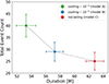 |
Fig. 11. Average duration and the number of plasmoid events for the three cases. Model A exhibits more frequent magnetic reconnection events, leading to more plasmoid events; however, radiative cooling also causes plasmoids to dissipate earlier, resulting in relatively short durations. |
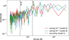 |
Fig. 12. Power spectral density of the plasmoid counts, obtained via temporal Fourier analysis for different cases. Vertical dashed lines mark the divisions between high- (0–50,M), mid- (50–150,M), and low- (> 150M) frequency bands. |
In the high-frequency range (0 − 50 M), the radiatively cooled case (model A) shows a higher average amplitude, indicating the occurrence of rapid reconnection events and radiatively driven plasmoid collapses. In contrast, the non-cooling model (model C) shows the highest average amplitude in the low-frequency range (greater than 150 M), suggesting a dominant contribution from the longer lifetime of plasmoid chains. As the strength of radiative cooling increases (from model B to model A), the average amplitude in the low-frequency band gradually decreases, implying that radiative collapse significantly shortens the duration of large-scale plasmoid events (see Table 2).
Mean amplitudes of plasmoid fluctuations in different frequency bands.
To further explore the impact of radiative cooling on the plasmoids, we analyzed and compared the radii of plasmoids detected in models A, B, and C, shown in Fig. 13. The results reveal that the layer compression caused by radiative cooling also affects plasmoids, resulting in a tendency toward the production of smaller plasmoids. The mean radius of models A, B, and C is r = 1.43, 1.59, and 1.80 GM/c2. It is reflected in the increase in the total number of plasmoids seen in Fig. 10.
 |
Fig. 13. Number counts of the detected plasmoid radii in different models: cooling with Ṁ/ṀEdd = 10−3 (green), cooling with Ṁ/ṀEdd = 10−5 (blue), and non-cooling (red). |
3.2.4. Magnetic field accumulation
Magnetic flux pile-up occurs when the rate of magnetic flux injection,  , exceeds that of flux annihilation in the reconnection layer, τR−1/τA−1 (Biskamp 1986). Here,
  and τR−1 are the flux injection and reconnection rates, respectively, τA is the Alfvén transit time, Vin is the inflow velocity, and VA, 1 and MA, 1 are the Alfvén velocity and Mach number in the inflow, respectively.
Due to the increased reconnection rate, as discussed in Sect. 3.2.3, a greater amount of magnetic flux undergoes annihilation along the current sheet, thereby reducing magnetic flux ΦBH. This explains the trend in magnetic flux variation observed in Fig. 1d, where stronger radiative cooling results in less magnetic flux accumulation. For larger magnetic loops, such as in models D, E, and F, we expect more magnetic field accumulation at the event horizon. As discussed in Sect. 3.1, radiative cooling suppresses the development of the MAD state. For instance, in model D, strong radiative cooling case, the magnetic field fails to reach the critical strength required to choke the accretion flow, and as a result, the MAD state does not emerge. Similarly, the weak radiative cooling in model E delays its entry into the MAD state compared to model F. Furthermore, the duration of each periodic MAD phase of the weak cooling case is noticeably shorter, which is reflected in sharper sawtooth-like structures in Fig. 1d. We attribute this to the reduced accumulation of magnetic fields (stronger magnetic flux annihilation) caused by radiative cooling. When the magnetic flux meets the threshold for the MAD state, the reduction in magnetic field strength quickly returns it to the SANE state soon.
3.2.5. Energy extraction
Plasmoid chain created by magnetic reconnection in BH ergosphere is one of the possible mechanisms of energy extraction from a rotating BH via the PP (e.g., Asenjo & Comisso 2015). In previous studies of reconnection-driven PP, the discussion has primarily focused on current sheets forming near the equatorial plane of the BH (Koide & Arai 2008; Asenjo & Comisso 2015). A recent study of Camilloni & Rezzolla (2025) has shown that PP can also occur outside the equatorial plane, as strong magnetic reconnection regions are present on the transition region between the accretion disk and the jet (Dimitropoulos et al. 2025). To precisely characterize PP, a local model of magnetic reconnection is required, providing a prescription for the plasmoid outflow velocity field  and their associated energetics. However, the quantities of greatest importance, outflow velocity and the reconnection rate, come from magnetohydrodynamic approximation (Shen & YuChih 2025; Camilloni & Rezzolla 2025). In our study, we did not pursue further theoretical analysis. Instead, we focused on how radiative cooling impact the energy extraction process via magnetic reconnection although it happens numerically due to numerical resistivity in ideal GRMHD simulations.
We then followed the definition provided in Shen & YuChih (2025), the energy conservation ∇μTtμ = 0, leading to the following form:
 (9)
(9)
where e = −αTtt denotes the so-called energy-at-infinity density. Here,  denotes the scale factor in the context of the 3 + 1 formalism, where gii represents the metric components in Boyer–Lindquist coordinates.
Figure 14 shows the distribution of energy-at-infinity density near the BH from our simulation of model A at t = 7330 M. As shown in the zoomed-in region, a negative energy density structure is embedded within a plasmoid. This feature arises from the tearing instability of the current sheet and subsequent magnetic reconnection near the plasmoid, leading to the formation of both negative and positive energy regions (Camilloni & Rezzolla 2025). One plasmoid carries negative energy and falls into the BH, while another carries positive energy and escapes outward. This bidirectional energy flow reflects a Penrose-like mechanism driven by reconnection. We note that only the escaping positive energy flux contributes to extracting energy from the BH, whereas negative energy falling inward contributes to the total energy budget without aiding extraction.
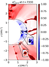 |
Fig. 14. Distribution of the normalized energy-at-infinity density (e∞) for model A within 3 rg at t = 7330 M. The dashed line indicates the position of ergosphere. The zoomed-in region shows two plasmoids: one associated with negative energy falling into the BH, and the other with positive energy escaping outward. |
To present directly that the plasmoid carrying negative energy-at-infinity falls into the BH, we tracked the evolution of a selected plasmoid near the equatorial plane, as shown in Fig. 15. The time evolution clearly shows the inward motion of the plasmoid with negative energy-at-infinity as it plunges into the BH.
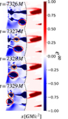 |
Fig. 15. Time evolution of the normalized energy-at-infinity density near the horizon around the equatorial plane for model A. The plasmoid with negative energy-at-infinity falls into the BH near the equatorial plane. The regions outlined in red and orange highlight two plasmoid chains with negative energy-at-infinity flowing inward. The dashed lines indicate the position of the ergosphere. |
As discussed in Sect. 3.2.3, radiative cooling affects the local reconnection rate and the efficiency of plasmoid formation. As shown in Fig. 16, we adopted previously introduced −hut as the diagnostic criterion to identify negative-energy regions within plasmoids, and compute the total negative energy by summing over these regions for each model. In model A (strong radiative cooling), two prominent peaks are observed around t = 14050 M and t = 14700 M. Similarly, in Fig. 10, peaks corresponding to plasmoid formation events are observed near these times, further supporting the temporal correlation. For model C (no cooling), although no prominent peaks are observed, there still exists noticeable variations corresponding to plasmoid formation events between t = 14200 M and t = 14600 M, compared to the surrounding periods. Model A exhibits a higher average negative energy-at-infinity density compared to the non-cooling model C. Thus, to some extent, radiative cooling can lead to more efficient energy extraction. Although a rigorous calculation of energy extraction requires a more detailed discussion, the trend-based analysis of negative energy differences across different models presented here provide supporting evidence for our discussion on the effects of radiative cooling.
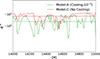 |
Fig. 16. Differences in the total negative energy among the different models. The horizontal dashed lines denote the average value of each model. |
4. Summary and discussion
We performed a series of 2D and 3D two-temperature GRMHD simulations initialized with a multi-loop configuration to systematically examine the effect of radiative cooling on the accretion flows. We focused on the cooling-induced collapse of plasmoids, analyzing their statistical properties under varying cooling strengths. We further investigated how these radiative-cooling-driven collapse events alter the small-scale structure of the current sheet and assessed their potential impact on energy extraction mechanisms. Below, we summarize our conclusions:
-
Radiative cooling significantly modifies the accretion dynamics near the BH, reducing the magnetic flux accumulation at the event horizon and influencing the transition between the SANE and MAD states.
-
Radiative cooling globally reduces the dimensionless electron temperature and increases the disk density through enhanced compression and alterations in the magnetic field structure, leading to observable modifications in the disk morphology.
-
Cooling induces layer compression within the reconnection regions, resulting in smaller plasmoid structures and promoting faster radiative collapse, thereby shortening the lifetime of individual plasmoid events.
-
Radiative cooling results in a higher frequency of plasmoid formation. However, the average “lifetime” of individual plasmoids decreases due to cooling-induced collapse. The radiative cooling case tends to have more small-scale reconnection events and radiative plasmoid collapses. The interplay between enhanced reconnection and rapid collapse maintains a similar average number of plasmoids.
-
A comparison of negative energy-at-infinity density variations under different radiative cooling conditions reveals the presence of peaks associated with plasmoid formation events. Radiative cooling may modulate the efficiency and characteristics of energy extraction to some extent.
Recent observations of rapid variability in X-ray and gamma-ray flares from active galactic nuclei, with timescales ranging from several minutes to a few hours, impose stringent constraints on particle acceleration timescales and the size of the emission region (Aharonian et al. 2007; Albert et al. 2007). Observational evidence suggests that these fast-variable flares originate from a compact region with a size on the order of a few Schwarzschild radii. Our results suggest that the collapse induced by radiative cooling confines plasmoid chains to smaller spatial regions and shortens their temporal duration. Therefore, our radiative cooling simulations may, to some extent, correspond to the observed variability in active galactic nuclei. The trends revealed by our results also offer a potential explanation for low-accretion-rate systems, such as Sgr A*.
Owing to limited computational resources, the presence of plasmoids cannot be resolved in our current 3D simulations, preventing us from modeling and tracking their temporal evolution. In future work, we plan to explore the impact of radiative cooling on the accretion process using higher-resolution, multi-loop 3D GRMHD simulations, with the goal of detecting and characterizing plasmoids in fully 3D settings. Moreover, the cooling model implemented in our simulations corresponds to a substantially higher accretion rate than that inferred for Sgr A*. At such accretion rates, of order Ṁ ∼ 10−3 ṀEdd, additional radiative processes–most notably inverse Compton scattering–as well as radiation back-reaction on the plasma dynamics may become dynamically important. Since these effects are not yet included in a fully self-consistent manner in our current cooling prescription, the quantitative details of the accretion-flow structure, plasmoid evolution, and energy-extraction efficiency may be affected. Consequently, our results should be regarded as indicative of qualitative trends rather than precise quantitative predictions at these accretion rates. In future studies, we plan to construct a more self-consistent cooling framework tailored to the physical conditions of Sgr A*, with the goal of better understanding its observed flaring behavior.
Acknowledgments
This research was supported by the National Key Research and Development Program of China (grant no. 2023YFE0101200), the National Natural Science Foundation of China (grant nos. 12273022, 12511540053), and the Shanghai Municipality Orientation Program of Basic Research for International Scientists (grant no. 22JC1410600). C.M.F. is supported by the DFG research grant “Jet physics on horizon scales and beyond” (Grant No. 443220636) within the DFG research unit “Relativistic Jets in Active Galaxies” (FOR 5195). The simulations were performed on the TDLI-Astro cluster at Shanghai Jiao Tong University.
References
- Aharonian, F., Akhperjanian, A. G., Bazer-Bachi, A. R., et al. 2007, A&A, 470, 475 [NASA ADS] [CrossRef] [EDP Sciences] [Google Scholar]
- Albert, J., Aliu, E., Anderhub, H., et al. 2007, ApJ, 663, 125 [Google Scholar]
- Antonopoulou, E., Loules, A., & Nathanail, A. 2025, A&A, 696, A10 [NASA ADS] [CrossRef] [EDP Sciences] [Google Scholar]
- Asenjo, F. A., & Comisso, L. 2015, Phys. Rev. Lett., 114, 115003 [Google Scholar]
- Biskamp, D. 1986, Phys. Fluids, 29, 1520 [Google Scholar]
- Camilloni, F., & Rezzolla, L. 2025, ApJ, 982, L31 [Google Scholar]
- Chael, A. 2025, MNRAS, 537, 2496 [Google Scholar]
- Chashkina, A., Bromberg, O., & Levinson, A. 2021, MNRAS, 508, 1241 [NASA ADS] [CrossRef] [Google Scholar]
- Chavez, E., Issaoun, S., Johnson, M. D., et al. 2024, ApJ, 974, 116 [Google Scholar]
- Christie, I. M., Petropoulou, M., Sironi, L., & Giannios, D. 2019, MNRAS, 482, 65 [Google Scholar]
- Del Zanna, L., Zanotti, O., Bucciantini, N., & Londrillo, P. 2007, A&A, 473, 11 [NASA ADS] [CrossRef] [EDP Sciences] [Google Scholar]
- Dibi, S., Drappeau, S., Fragile, P. C., Markoff, S., & Dexter, J. 2012, MNRAS, 426, 1928 [NASA ADS] [CrossRef] [Google Scholar]
- Dihingia, I. K., Mizuno, Y., Fromm, C. M., & Rezzolla, L. 2023, MNRAS, 518, 405 [NASA ADS] [Google Scholar]
- Dimitropoulos, I., Nathanail, A., Petropoulou, M., Contopoulos, I., & Fromm, C. M. 2025, A&A, 696, A36 [NASA ADS] [CrossRef] [EDP Sciences] [Google Scholar]
- Dorman, V. L., & Kulsrud, R. M. 1995, ApJ, 449, 777 [Google Scholar]
- Drappeau, S., Dibi, S., Dexter, J., Markoff, S., & Fragile, P. C. 2013, MNRAS, 431, 2872 [Google Scholar]
- El Mellah, I., Cerutti, B., & Crinquand, B. 2023, A&A, 677, A67 [NASA ADS] [CrossRef] [EDP Sciences] [Google Scholar]
- Esin, A. A., Narayan, R., Ostriker, E., & Yi, I. 1996, ApJ, 465, 312 [Google Scholar]
- Event Horizon Telescope Collaboration (Akiyama, K., et al.) 2022a, ApJ, 930, L12 [NASA ADS] [CrossRef] [Google Scholar]
- Event Horizon Telescope Collaboration (Akiyama, K., et al.) 2022b, ApJ, 930, L16 [NASA ADS] [CrossRef] [Google Scholar]
- Event Horizon Telescope Collaboration (Akiyama, K., et al.) 2024, ApJ, 964, L25 [NASA ADS] [CrossRef] [Google Scholar]
- Fan, Z.-Y., Li, Y., Zhou, F., & Guo, M. 2024, Phys. Rev. D, 110, 104044 [Google Scholar]
- Field, G. B. 1965, ApJ, 142, 531 [Google Scholar]
- Fishbone, L. G., & Moncrief, V. 1976, ApJ, 207, 962 [NASA ADS] [CrossRef] [Google Scholar]
- Forbes, T. G., & Malherbe, J. M. 1991, Sol. Phys., 135, 361 [NASA ADS] [CrossRef] [Google Scholar]
- Fragile, P. C., & Meier, D. L. 2009, ApJ, 693, 771 [CrossRef] [Google Scholar]
- Giulini, D. 2015, Gen. Rel. Grav., 47, 3 [Google Scholar]
- Gottlieb, O., Issa, D., Jacquemin-Ide, J., et al. 2023, ApJ, 954, L21 [Google Scholar]
- GRAVITY Collaboration (Abuter, R., et al.) 2018, A&A, 618, L10 [NASA ADS] [CrossRef] [EDP Sciences] [Google Scholar]
- GRAVITY Collaboration (Abuter, R., et al.) 2023, A&A, 677, L10 [NASA ADS] [CrossRef] [EDP Sciences] [Google Scholar]
- Grigorian, A. A., & Dexter, J. 2024, MNRAS, 530, 1563 [Google Scholar]
- Jiang, H.-X., Mizuno, Y., Fromm, C. M., & Nathanail, A. 2023, MNRAS, 522, 2307 [NASA ADS] [CrossRef] [Google Scholar]
- Jiang, H.-X., Mizuno, Y., Dihingia, I. K., et al. 2024, A&A, 688, A82 [NASA ADS] [CrossRef] [EDP Sciences] [Google Scholar]
- Jiang, H.-X., Mizuno, Y., Dihingia, I. K., et al. 2025, ApJ, 990, 81 [Google Scholar]
- Kaufman, E., Christie, I. M., Lalakos, A., Tchekhovskoy, A., & Giannios, D. 2023, ApJ, 954, 40 [Google Scholar]
- Kawazura, Y., Barnes, M., & Schekochihin, A. A. 2019, Proc. Nat. Acad. Sci., 116, 771 [NASA ADS] [CrossRef] [Google Scholar]
- Koide, S., & Arai, K. 2008, ApJ, 682, 1124 [Google Scholar]
- Kumar, D., Bhattacharyya, R., & Smolarkiewicz, P. K. 2015, Phys. Plasmas, 22, 012902 [Google Scholar]
- Lasota, J. P., Gourgoulhon, E., Abramowicz, M., Tchekhovskoy, A., & Narayan, R. 2014, Phys. Rev. D, 89, 024041 [NASA ADS] [CrossRef] [Google Scholar]
- Lin, X., & Yuan, F. 2024, MNRAS, 531, 3136 [NASA ADS] [CrossRef] [Google Scholar]
- Lin, X., Li, Y.-P., & Yuan, F. 2023, MNRAS, 520, 1271 [NASA ADS] [CrossRef] [Google Scholar]
- Liska, M., Tchekhovskoy, A., & Quataert, E. 2020, MNRAS, 494, 3656 [Google Scholar]
- Liska, M. T. P., Musoke, G., Tchekhovskoy, A., Porth, O., & Beloborodov, A. M. 2022, ApJ, 935, L1 [NASA ADS] [CrossRef] [Google Scholar]
- Loureiro, N. F., Samtaney, R., Schekochihin, A. A., & Uzdensky, D. A. 2012, Phys. Plasmas, 19, 042303 [NASA ADS] [CrossRef] [Google Scholar]
- Markoff, S., & Event Horizon Telescope Collaboration 2022, Am. Astron. Soc. Meeting Abstr., 240, 211.01 [Google Scholar]
- Mizuno, Y., Fromm, C. M., Younsi, Z., et al. 2021, MNRAS, 506, 741 [NASA ADS] [CrossRef] [Google Scholar]
- Narayan, R., & Yi, I. 1995, ApJ, 452, 710 [NASA ADS] [CrossRef] [Google Scholar]
- Narayan, R., Chael, A., Chatterjee, K., Ricarte, A., & Curd, B. 2022, MNRAS, 511, 3795 [NASA ADS] [CrossRef] [Google Scholar]
- Nathanail, A., Fromm, C. M., Porth, O., et al. 2020, MNRAS, 495, 1549 [Google Scholar]
- Nathanail, A., Mpisketzis, V., Porth, O., Fromm, C. M., & Rezzolla, L. 2022, MNRAS, 513, 4267 [NASA ADS] [CrossRef] [Google Scholar]
- Ni, L., Zhang, Q.-M., Murphy, N. A., & Lin, J. 2017, ApJ, 841, 27 [Google Scholar]
- Noble, S. C., Krolik, J. H., & Hawley, J. F. 2009, ApJ, 692, 411 [NASA ADS] [CrossRef] [Google Scholar]
- Olivares, H., Porth, O., Davelaar, J., et al. 2019, A&A, 629, A61 [NASA ADS] [CrossRef] [EDP Sciences] [Google Scholar]
- Penrose, R., & Floyd, R. M. 1971, Nat. Phys. Sci., 229, 177 [NASA ADS] [CrossRef] [Google Scholar]
- Petropoulou, M., Giannios, D., & Sironi, L. 2016, MNRAS, 462, 3325 [NASA ADS] [CrossRef] [Google Scholar]
- Porth, O., Olivares, H., Mizuno, Y., et al. 2017, Comput. Astrophys. Cosmol., 4, 1 [Google Scholar]
- Porth, O., Chatterjee, K., Narayan, R., et al. 2019, ApJS, 243, 26 [Google Scholar]
- Porth, O., Mizuno, Y., Younsi, Z., & Fromm, C. M. 2021, MNRAS, 502, 2023 [NASA ADS] [CrossRef] [Google Scholar]
- Ressler, S. M., Tchekhovskoy, A., Quataert, E., Chandra, M., & Gammie, C. F. 2015, MNRAS, 454, 1848 [Google Scholar]
- Ripperda, B., Porth, O., Xia, C., & Keppens, R. 2017, MNRAS, 467, 3279 [NASA ADS] [Google Scholar]
- Ripperda, B., Porth, O., Sironi, L., & Keppens, R. 2019, MNRAS, 485, 299 [CrossRef] [Google Scholar]
- Ripperda, B., Liska, M., Chatterjee, K., et al. 2022, ApJ, 924, L32 [NASA ADS] [CrossRef] [Google Scholar]
- Rodman, P. E., & Reynolds, C. S. 2024, ApJ, 960, 97 [Google Scholar]
- Ryan, B. R., Ressler, S. M., Dolence, J. C., Gammie, C., & Quataert, E. 2018, ApJ, 864, 126 [CrossRef] [Google Scholar]
- Sądowski, A., Wielgus, M., Narayan, R., et al. 2017, MNRAS, 466, 705 [NASA ADS] [CrossRef] [Google Scholar]
- Salas, L. D. S., Liska, M. T. P., Markoff, S. B., et al. 2025, MNRAS, 538, 698 [Google Scholar]
- Scepi, N., Dexter, J., & Begelman, M. C. 2022, MNRAS, 511, 3536 [NASA ADS] [CrossRef] [Google Scholar]
- Shen, Y., & YuChih, H.-Y. 2025, Phys. Rev. D, 111, 023003 [Google Scholar]
- Singh, A., Bégué, D., & Pe’er, A. 2025, ApJ, 981, L11 [Google Scholar]
- Tchekhovskoy, A., McKinney, J. C., & Narayan, R. 2009, ApJ, 699, 1789 [NASA ADS] [CrossRef] [Google Scholar]
- Tchekhovskoy, A., Narayan, R., & McKinney, J. C. 2011, MNRAS, 418, L79 [NASA ADS] [CrossRef] [Google Scholar]
- Trippe, S., Paumard, T., Ott, T., et al. 2007, MNRAS, 375, 764 [NASA ADS] [CrossRef] [Google Scholar]
- Uzdensky, D. A., & McKinney, J. C. 2011, Phys. Plasmas, 18, 042105 [NASA ADS] [CrossRef] [Google Scholar]
- Van der Walt, S., Schönberger, J. L., Nunez-Iglesias, J., et al. 2014, PeerJ, 2, e453 [Google Scholar]
- Yoon, D., Chatterjee, K., Markoff, S. B., et al. 2020, MNRAS, 499, 3178 [NASA ADS] [CrossRef] [Google Scholar]
- Yuan, F., Quataert, E., & Narayan, R. 2004, ApJ, 606, 894 [Google Scholar]
- Zhang, H., Li, X., Guo, F., & Giannios, D. 2018, ApJ, 862, L25 [NASA ADS] [CrossRef] [Google Scholar]
Appendix A: Radiative cooling terms
The total cooling rate for an optically thin gas is determined as
 (A.1)
(A.1)
where ηC denotes the Compton enhancement factor, which is explicitly given as Narayan & Yi (1995)
 (A.2)
(A.2)
The terms in the Compton enhancement factor are defined as follows: P = 1 − exp(−τes), A = 1 + 4Θe + 16Θe2, η1 = 1 + lnP/lnA, τes = 2σTneH. Where σT is the Thomson cross section of the electron, ne is the electron number density, H is the local scale height.
To compute the bremsstrahlung cooling rate, we adopted the formulations presented by Esin et al. (1996). Specifically, the free-free bremsstrahlung cooling rate for an ionized plasma, consisting of electrons and ions, is expressed as
 (A.3)
(A.3)
where the explicit forms of the individual components are given by
![Mathematical equation: $$ \begin{aligned}&q_{\text{br}}^{ei} = 1.48 \times 10^{-22} n_i n_e \times \nonumber \\&\left\{ \begin{array}{ll} \displaystyle \frac{4\sqrt{2\Theta _e}}{\pi ^{3/2}} \left(1 + 1.781 \Theta _e^{1.34}\right),&\Theta _e < 1 \\ \displaystyle \frac{9\Theta _e}{2\pi } \left[\ln (1.123\Theta _e) + 0.48\right] + 1.5,&\text{ otherwise;} \text{ and} \end{array} \right. \end{aligned} $$](/articles/aa/full_html/2026/03/aa57948-25/aa57948-25-eq23.gif) (A.4)
(A.4)
![Mathematical equation: $$ \begin{aligned} q_{\text{br}}^{ee} = \left\{ \begin{array}{ll} \displaystyle 2.56 \times 10^{-22} \, n_e^2 \Theta _e^{3/2} \left(1 + 1.1\Theta _e + \Theta _e^2 - 1.25\Theta _e^{5/2} \right),&\Theta _e < 1 \\ \displaystyle 3.24 \times 10^{-22} \, n_e^2 \Theta _e \left[\ln (1.123\Theta _e) + 1.28\right],&\text{ otherwise.} \end{array} \right. \end{aligned} $$](/articles/aa/full_html/2026/03/aa57948-25/aa57948-25-eq24.gif) (A.5)
(A.5)
Here, Θe := kBTe/mec2 is the dimensionless electron temperature.
In the presence of a strong magnetic field, the hot electrons in the accretion flow radiate via the thermal synchrotron process. The rate of synchrotron emission, as formulated by Esin et al. (1996), is expressed as
![Mathematical equation: $$ \begin{aligned} q^-_{\text{cs}}&= \frac{2\pi k_B T_i \nu _c^3}{3 H c^2} + 6.76 \times 10^{-28} \frac{n_e}{K_2(1/\Theta _e) a_1^{1/6}}\times \nonumber \\&\left[\frac{1}{a_4^{11/2}} \Gamma \left(\frac{11}{2}, a_4 \nu _c^{1/3}\right) + \frac{a_2}{a_4^{19/4}} \Gamma \left(\frac{19}{4}, a_4 \nu _c^{1/3}\right) \right. \\&\left. + \frac{a_3}{a_4^4} \left(a_3^4 \nu _c + 3a_2^2 \nu _c^{2/3} + 6a_4 \nu _c^{1/3} + 6\right) e^{-a_4 \nu _c^{1/3}} \right] \nonumber , \end{aligned} $$](/articles/aa/full_html/2026/03/aa57948-25/aa57948-25-eq25.gif) (A.6)
(A.6)
where H is the local scale height, estimated from the gradient of the electron temperature as H = Te4 / |∇Te4|. The function K2 represents the modified Bessel function of the second kind. The coefficients a1 through a4 in Eq. A.6 are as defined in Esin et al. (1996).
Appendix B: Resolution test
To investigate the effects of numerical resolution, we conducted 2D GRMHD simulations of magnetized accretion flows onto a rotating BH, incorporating radiative cooling, at different grid resolutions. Model hr has the same initial condition as model A, differing only in resolution. We adopted a grid size of (Nr, Nθ) = 1024 × 512 as the standard resolution and We adopted five levels of static mesh refinement with a base resolution of (Nr, Nθ) = 256 × 128. The second refinement level is applied within the radial range 100 < r/rg < 200, the third within 90 < r/rg < 100, the fourth within 60 < r/rg < 90, and the fifth within 3 < r/rg < 60. As a result, the effective resolution in the regions of prime interest reaches (Nr, Nθ) = 4096 × 2048, allowing us to capture the dynamics near the current sheet with significantly enhanced spatial resolution. As shown in Fig. B.1, the evolutionary trends between different resolution cases show excellent agreement.
In the meanwhile, we also observed radiative collapse induced by radiative cooling, shown in Fig. B.2. This confirms that radiative collapse is a general and resolution-insensitive feature of the system, rather than a numerical artifact.
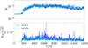 |
Fig. B.1. Time evolution of the mass accretion rate (top panel) and the magnetic flux (bottom panel) for model A and the high-resolution model (hr). |
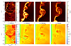 |
Fig. B.2. Distribution of electron temperature and density at standard resolution. |
All Tables
Model parameters: λr, the mass accretion rate normalized by the Eddington ratio, the radiative cooling status, and the grid number.
All Figures
|
Fig. 1. Time evolution of mass accretion rates measured at the event horizon (top) and the normalized magnetic flux at the horizon (bottom). Panels (a) and (c): Case with smaller magnetic loops (λ = 40). Panels (b) and (d): Case with larger magnetic loops (λ = 80). The curves in different colors correspond to the different radiative cooling and time-averaged accretion rates: radiative cooling with Ṁ/ṀEdd = 1 × 10⁻³ (blue and green), radiative cooling with 1 × 10⁻⁵(black and light blue), and no cooling (red and light red). In panel (c), the horizontal red and blue lines denote the average magnetic flux of models A and C, respectively. The blue vertical lines in panels (a) and (c) mark the onset of the quasi-steady state. In panels (b) and (d), the light blue and light red vertical lines indicate the transition from SANE to MAD for models E and F, respectively. The time is given in units of the light crossing time, tg ≡ GM/c3 = [M]. |
| In the text | |
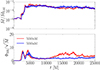 |
Fig. 2. Same as Fig. 1 but shown for 3D cases (M40n3d and M40a3d). |
| In the text | |
|
Fig. 3. Time-averaged electron temperature (Θe), plasma β, and density (ρ) distributions for models A, B, and C (from top to bottom). The plasma beta parameter is defined as β = pg/pmag, where pg represents the gas pressure, and pmag = b2/2 denotes the magnetic pressure. The black contours in the density profile represent the magnetic field. The average is taken over the time range t = 8000 M to 13 000 M. |
| In the text | |
|
Fig. 4. Density-weighted scale height as a function of radius for cooling models A, B, and C. |
| In the text | |
|
Fig. 5. Azimuthal and time-averaged polar-angle profiles of the ion-to-electron temperature ratio of models A, B, and C at r = 15 M. The averaging time range is the same as used in Fig. 3. |
| In the text | |
|
Fig. 6. Distribution of the time-averaged density and electron temperature at ϕ = 0 for the models (with cooling and without cooling) in the averaging range t = 10000 M–14000 M. |
| In the text | |
|
Fig. 7. Distribution of the axial component of the magnetic field (Bz) in a cross-sectional slice at t = 7920 M for models M40a3d (left) and M40n3d (right). |
| In the text | |
|
Fig. 8. Time evolution of a plasmoid chain in the high-resolution model hr over the time interval t = 8170 M to t = 8180 M. Upper panel: Electron temperature. Lower panel: Density. We mark the location of the plasmoid chain with a red box in each panel. |
| In the text | |
|
Fig. 9. Time evolution of the integrated density (blue) and electron temperature (red) of a tracked plasmoid in the interval shown in Fig. 8. |
| In the text | |
|
Fig. 10. Time evolution of the number of detected plasmoids in different models: cooling with Ṁ/ṀEdd = 10−3(top), cooling with Ṁ/ṀEdd = 10−5 (middle), and non-cooling (bottom). |
| In the text | |
|
Fig. 11. Average duration and the number of plasmoid events for the three cases. Model A exhibits more frequent magnetic reconnection events, leading to more plasmoid events; however, radiative cooling also causes plasmoids to dissipate earlier, resulting in relatively short durations. |
| In the text | |
|
Fig. 12. Power spectral density of the plasmoid counts, obtained via temporal Fourier analysis for different cases. Vertical dashed lines mark the divisions between high- (0–50,M), mid- (50–150,M), and low- (> 150M) frequency bands. |
| In the text | |
|
Fig. 13. Number counts of the detected plasmoid radii in different models: cooling with Ṁ/ṀEdd = 10−3 (green), cooling with Ṁ/ṀEdd = 10−5 (blue), and non-cooling (red). |
| In the text | |
|
Fig. 14. Distribution of the normalized energy-at-infinity density (e∞) for model A within 3 rg at t = 7330 M. The dashed line indicates the position of ergosphere. The zoomed-in region shows two plasmoids: one associated with negative energy falling into the BH, and the other with positive energy escaping outward. |
| In the text | |
|
Fig. 15. Time evolution of the normalized energy-at-infinity density near the horizon around the equatorial plane for model A. The plasmoid with negative energy-at-infinity falls into the BH near the equatorial plane. The regions outlined in red and orange highlight two plasmoid chains with negative energy-at-infinity flowing inward. The dashed lines indicate the position of the ergosphere. |
| In the text | |
|
Fig. 16. Differences in the total negative energy among the different models. The horizontal dashed lines denote the average value of each model. |
| In the text | |
|
Fig. B.1. Time evolution of the mass accretion rate (top panel) and the magnetic flux (bottom panel) for model A and the high-resolution model (hr). |
| In the text | |
|
Fig. B.2. Distribution of electron temperature and density at standard resolution. |
| In the text | |
Current usage metrics show cumulative count of Article Views (full-text article views including HTML views, PDF and ePub downloads, according to the available data) and Abstracts Views on Vision4Press platform.
Data correspond to usage on the plateform after 2015. The current usage metrics is available 48-96 hours after online publication and is updated daily on week days.
Initial download of the metrics may take a while.