| Issue |
A&A
Volume 707, March 2026
|
|
|---|---|---|
| Article Number | A142 | |
| Number of page(s) | 15 | |
| Section | Galactic structure, stellar clusters and populations | |
| DOI | https://doi.org/10.1051/0004-6361/202557996 | |
| Published online | 11 March 2026 | |
Cepheid Metallicity in the Leavitt Law (C- MetaLL) survey
VIII. Spectroscopic detection of rare earth dysprosium, erbium, lutetium, and thorium in classical Cepheids
1
INAF-Osservatorio Astronomico di Capodimonte,
Salita Moiariello 16,
80131
Naples,
Italy
2
INAF-Osservatorio Astrofisico di Catania,
Via S.Sofia 78,
95123
Catania,
Italy
3
Università di Salerno, Dipartimento di Fisica “E.R. Caianiello”,
Via Giovanni Paolo II 132,
84084
Fisciano (SA),
Italy
4
INAF-Osservatorio di Astrofisica e Scienza dello Spazio,
Via Gobetti 93/3,
40129
Bologna,
Italy
5
Leibniz-Institut für Astrophysik Potsdam (AIP),
An der Sternwarte 16,
14482
Potsdam,
Germany
6
Inter-University Center for Astronomy and Astrophysics (IUCAA),
Post Bag 4, Ganeshkhind,
Pune
411 007,
India
7
Istituto Nazionale di Fisica Nucleare (INFN)-Sez. di Napoli, Via Cinthia,
80126
Napoli,
Italy
8
European Southern Observatory,
Karl-Schwarzschild-Strasse 2,
85748
Garching bei München,
Germany
9
Scuola Superiore Meridionale,
Largo San Marcellino10
80138
Napoli,
Italy
10
INAF – Osservatorio Astronomico di Roma,
via Frascati 33,
00078
Monte Porzio Catone,
Italy
★ Corresponding author: This email address is being protected from spambots. You need JavaScript enabled to view it.
Received:
6
November
2025
Accepted:
9
January
2026
Abstract
Context. Classical Cepheids (DCEPs) are among the most important distance calibrators thanks to the correlation between their period and luminosity (PL relation), and play a crucial role in the calibration as the first rung of the extragalactic distance ladder. Given their typical age, they also constitute an optimal tracer of the young population in the Galactic disc.
Aims. We aim to increase the number of available DCEPs with high-resolution spectroscopic metallicities, study the galactocentric radial gradients of several chemical elements, and analyse the spatial distribution of the Galactic young population of stars in the Milky Way disc.
Methods. We performed a complete spectroscopical analysis of 136 spectra obtained from three different high-resolution spectrographs, for a total of 60 DCEPs. More than half have pulsational periods longer than 15 days, up to 70 days, doubling the number of stars in our sample with P > 15d. We derived radial velocities, atmospheric parameters, and chemical abundances for up to 33 different species.
Results. We present an updated list of trusted spectroscopic lines for the detection and estimation of chemical abundances. We used this new set to revisit the abundances already published in the context of the C-MetaLL (Cepheids-Metallicity in the Leavitt Law) survey and increase the number of available chemical species. For the first time (to our knowledge), we present the estimation of abundances for Cepheids for dysprosium (Dy, Z = 66), as well as a systematic estimation of erbium (Er, ZZ = 68), lutetium (Lu, Z = 71), and thorium (Th, Z = 90) abundances.
Conclusions. We calculated a galactic radial gradient for [Fe/H] with a slope of −0.064 ± 0.002 dex kpc−1, in good agreement with recent literature estimation. The other elements also exhibit a clear negative radial trend, with this effect diminishing and eventually disappearing for heavier neutron-capture elements. Depending on the proposed spiral arms model present in several literature sources, our most external stars agree on tracing either the Perseus, the Norma-Outer, or both the Outer and the association Outer-Scutum-Centaurus arms.
Key words: stars: abundances / stars: distances / stars: fundamental parameters / stars: variables: Cepheids / Galaxy: disk
© The Authors 2026
 Open Access article, published by EDP Sciences, under the terms of the Creative Commons Attribution License (https://creativecommons.org/licenses/by/4.0), which permits unrestricted use, distribution, and reproduction in any medium, provided the original work is properly cited.
This article is published in open access under the Subscribe to Open model. This email address is being protected from spambots. You need JavaScript enabled to view it. to support open access publication.
1 Introduction
Classical Cepheids (DCEPs) have been proven to play a fundamental role as standard candles, thanks to their relation between pulsational period and luminosity (PL relation, Leavitt & Pickering 1912). The calibration of this relation, or its reddening-free version, the period-Wesenheit (PW, Madore 1982) relation, through independent distance estimation using geometric methods such as trigonometric parallaxes, eclipsing binaries, and water masers, allows for the determination of distances of faraway objects, such as galaxies containing both DCEPs and type Ia supernovae. This further allows for the measurement of distances of more distant galaxies in the steady Hubble flow and eventually of one of the most important astrophysical parameters, the Hubble constant (H0). This parameter conceals within its value information on both the acceleration of the Universe and its age, making its determination with at least a 1% precision of extreme importance in modern astrophysics. Nowadays, several estimations are offered in the literature, exploring different methods. While the Planck mission, with the study of the cosmic microwave background under the assumption of the Λ cold dark matter (ΛCDM) cosmological model obtained H0 = 67.4±0.5 km s−1 Mpc−1 (Planck Collaboration VI 2020), the Supernovae, H0, for the Equation of State of Dark energy (SH0ES) project, using the cosmic distance ladder, estimated H0 = 73.01±0.99 km s−1 Mpc−1 (Riess et al. 2022). No solution has yet been reached for this 5σ discrepancy, but other empirical methods were proposed to analyse possible systematics in the calibration of the cosmic distance ladder, based either on replacing DCEPs with other astronomical objects, such as asymptotic giant branch stars (Lee et al. 2025; Li et al. 2025), the tip of the red giant branch (Hoyt et al. 2025), and Miras (Bhardwaj et al. 2025), or on replacing both the DCEPs and type Ia supernovae with red giant branch stars and surface brightness fluctuations (Anand et al. 2025), respectively. The metallicity dependence of PL/PW relations (also called PLZ/PWZ relations) may play a crucial role as a source of uncertainty (e.g. see recent discussion in Riess et al. 2021; Bhardwaj et al. 2023; Madore & Freedman 2025; Breuval et al. 2025). In this context, we initiated a project named Cepheid - Metallicity in the Leavitt Law (C-MetaLL, see Ripepi et al. 2021), whose main aim is to collect high-resolution galactic DCEP spectra and build a sample of more than 400 targets with spectroscopic metallicities estimated homogeneously (Ripepi et al. 2021; Trentin et al. 2023, 2024). High-resolution spectroscopy is also being complemented with homogeneous time-series photometry at multiple wavelengths in our survey (e.g. Bhardwaj et al. 2024). In particular, it is essential to obtain a dataset of targets well distributed in both metallicities and the period range to cover all the phase space for the calibration of the PLZ relations.
Our project has been very successful in increasing the number of DCEPs with low metallicity (see Trentin et al. 2023, 2024), but there is still a need to increase the number of stars with periods longer than 15 days. Beyond their role in the construction of the cosmic distance ladder, DCEPs are useful tracers of young population stars. In this role, they have also been used in the Milky Way (MW) (see e.g. Bono et al. 2024, for a recent review of the role of DCEPs in the Galaxy), and several recent studies have focused on the use of DCEPs to study the chemical distribution and the spiral structure of the MW (Luck & Lambert 2011; Genovali et al. 2014; Luck 2018; Lemasle et al. 2018; Skowron et al. 2019; Minniti et al. 2020; Ripepi et al. 2021; Lemasle et al. 2022; Kovtyukh et al. 2022; da Silva et al. 2023; Trentin et al. 2023; Matsunaga et al. 2023; Trentin et al. 2024; Drimmel et al. 2025; De Somma et al. 2025, and reference therein). The possibility of estimating chemical abundances for several elements, ranging from light elements such as carbon and oxygen up to heavy elements produced by neutron capture events such as yttrium (Y), barium (Ba), and europium (Eu), offers a unique opportunity to study the origin of these elements and discriminate different nucleosynthesis channels (see e.g. Kobayashi et al. 2020, and reference therein). This is the eighth paper within the C-MetaLL project and the fourth in which we present new observations and spectroscopic data to enlarge the sample of DCEPs with homogeneous high-resolution metallicities (see also Ripepi et al. 2021; Trentin et al. 2023, 2024). The structure of the paper is as follows: in Sect. 2, we describe the sample of new DCEPs; in Sect. 3, we describe the procedure to estimate both the atmospheric parameters and abundances; results are presented and discussed in Sects. 4 and 5, respectively. We give our conclusion in Sect. 6.
2 Observations and data reduction
In the context of the C-MetaLL survey, the observations were collected using three different instruments:
A sample of 23 stars (29 spectra in total) were observed at the European Southern Observatory (ESO) during period P112 (2023-2024) under proposal 112.25 NA. We used the Ultraviolet and Visual Echelle Spectrograph (UVES, Dekker et al. 2000)1, attached to Unit Telescope 2 (UT2) of the Very Large Telescope (VLT), placed at Paranal (Chile). The red arm was used, equipped with the grism CD#3, covering the wavelength interval 4760–6840 Å, and with the central wavelength at 5800 Å. The 1 arcsec slit, which provides a dispersion of R ~ 47 000 (sampling 2 px), was selected for all the targets. The number of epochs obtained with this instrument is typically 1–2.
A sample of 15 stars (for a total of 44 spectra) was observed with the High Accuracy Radial velocity Planet Searcher for the Northern hemisphere (HARPS-N, Mayor et al. 2003; Cosentino et al. 20122), at the 3.5 m Telescopio Nazionale Galileo (TNG), during period 47 (proposal A47TAC_18, July-August 2024). HARPS-N features an echelle spectrograph covering the wavelength range between 3830 and 6930 Å, with a spectral resolution of R=115 000 (sampling 3.3 px). Three or more epochs were obtained with HARPS-N for each object.
A sample of 22 stars (for a total of 63 spectra) was observed with the Potsdam Echelle Polarimetric and Spectroscopic Instrument (PEPSI, Strassmeier et al. 2015), the fibre-feed high-resolution optical echelle spectrograph for the Large Binocular Telescope (LBT). The observations were carried out in two periods (proposals IT-2019B-014 and IT-2021_2022_24) in 2019-2020 and 2021-2022. The wavelength coverage is between 4750 and 7430 Å, with a spectral resolution of R=50 000. Up to four epochs were obtained for each star with this instrument.
Reduction of all the spectra, which included bias subtraction, spectrum extraction, flat-fielding, and wavelength calibration, was done by automatic pipelines provided by the three instrument teams, so that we downloaded the science-ready one-dimensional spectra. For more details on the data reduction of HARPS-N, UVES spectra, see Ripepi et al. (2021) and Trentin et al. (2023), respectively. The PEPSI data were reduced using the PEPSI ‘Software for Stellar Spectroscopy’ (SDS4PEPSI Strassmeier et al. 2018).
Table A.1 lists the main properties of the target stars (RA, Dec., Period, pulsational mode, Gaia photometry and galactocentric polar coordinates), while the heliocentric Julian day (HJD) of observation, the exposure time and the signal-to-noise ratio (S/N) for each spectrum are shown in Table A.2.
The procedure to estimate some of the listed quantities in Table A.1 is described in Gaia Collaboration (2023a) and Ripepi et al. (2022). In summary, we calculated both the apparent Wesenheit magnitude W = G − 1.90 × (GBP − GRP) using the Gaia photometry (Ripepi et al. 2019) and the absolute W magnitude from the PWZ relation W = (−5.988 ± 0.018) − (3.176 ± 0.044)(log P − 1) − (0.520 ± 0.09)[Fe/H] (Ripepi et al. 2022). This way, it was possible to obtain the distance modulus, and so the distance. We converted the coordinates into the Galactocentric system, adopting R0 = 8277 ± 9(stat) ±30(sys) pc as the distance of the Sun from the Galactic centre (Gravity Collaboration 2022).
Some stars were also observed previously within the C-MetaLL project, and their abundances published elsewhere. In more detail:
TX Sct, ASAS-SN-J193606.44+215011.4, and ET Vul were already observed with HARPS-N, and had abundances published in Ripepi et al. (2021) and Trentin et al. (2024).
V459 Sct, V480 Aql, OGLE-GD-CEP-0604, and OGLE-GD-CEP-0841 were observed with UVES during ESO P105 (the first two), P109 and P110, respectively. Abundances were published in Trentin et al. (2023) and Trentin et al. (2024).
These stars are treated similarly to other stars with multiple observations (see Sect. 3.2) and, when observed with multiple instruments, represent a further test for confirming that there is no bias in the abundances.
Two stars, Gaia DR2 4638315266636230400 and Gaia DR2 4644478166748030976 (also known as OGLE SMC-CEP-4986 and OGLE SMC-CEP-4953, respectively), are not MW stars. Their spectral analysis will be included in this work, but the targets will be excluded from the results unless specifically mentioned (see Sect. 4). We note that 38 objects have periods longer than 15 d, for a maximum of 70 days. These objects are particularly useful, as they are rarer than the short-period ones and crucial to defining the PL/PW relations over a large range of periods. The distribution of the whole sample of stars included in the C-MetaLL project is displayed in Fig. 1.
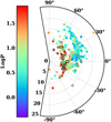 |
Fig. 1 Distribution of the C-MetaLL sample along the Galactic disc. The points are colour-coded according to the pulsator’s period. Targets presented in this work are highlighted with black borders. The position of the sun is shown with a yellow-black circle. |
3 Data analysis
3.1 Stellar parameters
The procedure and steps for both atmospheric parameters and chemical abundances estimation are the same as those reported in Ripepi et al. (2021); Trentin et al. (2023, 2024). The atmospheric parameters that need to be estimated are the effective temperature (Teff), surface gravity (log g), microturbulent velocity (ξ), and the joint effect of macroturbulence and rotational velocity, called the line-broadening parameter (Vbroad). A diffused method used to estimate the effective temperature, regardless of the interstellar reddening, is the line depth ratio (LDR) method (Gray & Johanson 1991; Kovtyukh & Gorlova 2000), with around 32 available LDRs per spectrum. To estimate ξ, we first measured the equivalent widths (EWs) of Fe I with a semi-automatic Python routine. As neutral Fe is insensitive to log g, it is possible to construct atmospheric models, using ATLAS9 (Kurucz 1993), by fixing Teff and log g and choosing a value of ξ. Thanks to the WIDTH9 code (Kurucz & Avrett 1981), it is possible to convert the EWs to abundances. We extrapolated the value of ξ for which the iron abundance is independent of EWs. Lastly, log g was estimated by imposing that the iron abundance from Fe II lines is the same as the one obtained with Fe I lines. The list of 145 Fe I and 24 Fe II lines was extracted from Romaniello et al. (2008). Errors for ξ and log g were obtained by error propagation from the linear fits ([Fe/H] versus EWs and [Fe II/H] versus log g, respectively). In Table A.2 we report all the useful parameters used as inputs for the abundance analysis of the 136 spectra analysed in this paper and presented in the next section.
3.2 Abundances
A spectral synthesis technique was used in order to avoid line-blending problems caused by line broadening. The technique is divided into three steps: (i) generation of plane-parallel local thermodynamic equilibrium (LTE) atmospheric models using the ATLAS9 code; (ii) synthesis of stellar spectra through SYNTHE (Kurucz & Avrett 1981); (iii) convolution of the synthetic spectra to take into account instrumental and line broadening. By matching the synthetic line to a selected set of observed metal lines, it is possible to evaluate this last parameter. We divided the observed spectra into intervals of variable width (from 10 to 50 Å, depending on the region of the spectrum) and performed a χ2 minimisation of the differences between observed and synthetic spectra to derive the chemical abundances. The algorithm, written in Python, is based on multi-dimensional minimisation of a function using the downhill simplex method (Nelder & Mead 1965). Up to 32 different chemical species were estimated for each spectrum. The error on the single measurement was obtained by evaluating the uncertainties caused by varying the atmospheric parameters. For variations of δTeff= ±150 K, δ log g = ±0.2 dex, and δξ = ±0.3 km s−1, we estimated a total contribution to the error of ≈ ±0.1 dex. When a single spectral line was detected for an element, we propagated the errors of the atmospheric parameters; otherwise, we averaged the abundance and propagated the errors. We used the lists of spectral lines and atomic parameters from Castelli & Hubrig (2004), which updated the original parameters from Kurucz (1995). When necessary, we also checked the NIST database (Ralchenko & Reader 2019). Solar values used as a reference are from Asplund et al. (2021). We evaluated the impact of non-LTE correction on our results using the grids published in Amarsi et al. (2020), which explored a wide range of non-LTE corrections for several elements. In particular, according to the low metallicity of our targets, we neglected corrections for carbon, magnesium, silicon, calcium, and barium, while we applied a correction of 0.1 dex on our LTE sodium abundance.
4 Results
4.1 Spectral lines detected and abundances
In this section, we present the list of spectral lines through which it was possible to estimate up to 32 different chemical species in the final phase of the spectral analysis and discuss the estimated abundances. This list, shown in Table A.3, is updated from the one already presented in Ripepi et al. (2021); Trentin et al. (2023). It is worth noting that for some elements (such as silicon, sulphur, scandium, cobalt, cerium, praseodymium, europium) the number of available lines is sensibly increased (if not doubled); for others (such as titanium and neodymium), several lines are available almost along the whole spectrum and we reported the most isolated and/or the strongest ones. In the last column of Table A.3, a brief note on each line was added, specifying whether it is a new line (‘New’) and if it was typically found partially blended with another line (‘Blend’ or ‘New,Blend’ to distinguish between the old and new lines, respectively). In the latter case, the estimated abundances were taken into consideration whenever the blending was not extreme and/or when no other line could be found for that element. Since metal-poor stars are also the farthest ones (see next section), not all the lines are always available, and their spectra are more affected by noise. On this basis, we expect that the increased number of available spectral lines might affect the results in the metal-poor regime. An example is shown in Fig. 2 for the Zinc case. While before only one weak line at λ 6362.338 Å (right panel) was available for the spectra obtained with UVES, a stronger line at λ 4810.532 Å (left panel) is now preferred. For these reasons, and to maintain the homogeneity in our analysis, we also re-estimated the abundances of the whole sample of stars previously published in the context of the C-MetaLL project, namely 290 stars, whose abundances have been published in Trentin et al. (2024). The final list of abundances for the entire dataset, i.e. including both the stars analysed in this work and those from our previous papers, is reported in Table A.4. This is the baseline data that will be used in the following.
When comparing our previously published abundances with those obtained with the updated list we note that, for most of the elements (e.g. oxygen, carbon, vanadium, titanium, barium) the differences are minimal (below 0.1 dex); for others (scandium, copper, zinc, yttrium, zirconium), most of the metal-poorer stars (with [Fe/H]<−0.4 dex) present differences up to 0.2–0.4 dex. This is evident when comparing Fig. 3, where we plot the abundances (in their [X/Fe] form) versus the iron abundance (in the [Fe/H] form), with Fig. 5 of Trentin et al. (2024). For these five elements, the discrepancy at low metallicities (yellow and red points, mostly observed with UVES) between the sample presented in Trentin et al. (2023) and Trentin et al. (2024) is reduced and less evident. For the heaviest elements, i.e. from barium onwards, elements previously not found in the sample presented in Trentin et al. (2023) were estimated (see the yellow points for cerium, samarium, europium, and gadolinium and the red points for samarium only). Lastly, we detected for the first time four new chemical elements: dysprosium (Dy, atomic number 66), erbium (Er, atomic number 68), lutetium (Lu, atomic number 71), and thorium (Th, atomic number 90).
The trends of each element with respect to iron are similar to those previously found in Trentin et al. (2024). In more detail:
C, O: For these elements, we found a descending trend with increasing metallicity, with over-solar values for [Fe/H] <−0.5 dex and sub-solar values for [Fe/H]> 0.2 dex. In between, both elements are almost constant, with carbon at ≈−0.1 [C/Fe] dex and oxygen at solar values. Three new spectral lines were found for C (at λ = 6014.830 Å) and oxygen (at λ = 5577.339 Å and 6363.776 Å);
Odd-Z elements (Na and Al): sodium was found to be constant along the whole metallicity range, at around 0.4 dex, while aluminium decreases at a constant pace, with [X/Fe] ≈0 dex for solar metallicity;
α elements (Mg, Si, S, Ca): all these elements show a decrease in their abundances with increasing iron, and flatten at [Fe/H] ≈ −0.5 dex. Two lines have been added for both magnesium and sulphur, while several new lines have been found for silicium and calcium (see Table A.3);
Scandium shows a peculiar behaviour, with a decreasing trend at low [Fe/H], a flattening at [Sc/Fe] ≈ 0.4 dex, and a hint of increasing again at higher metallicities ([Fe/H] > 0.2 dex). Two new lines at λ = 5641.001 and 5667.136 Å were found, plus a strong blended line at λ = 5657.875 Å;
Iron-peak elements (from Ti to Zn): most of the iron-peak elements (titanium, vanadium, chromium, cobalt, and nickel) show a trend similar to the one described for the α elements, while manganese and zinc remain relatively constant for the whole iron range. Copper shows a different behaviour, with a flattened value (≈0.4 dex at low metallicity and then starts decreasing at [Fe/H] ≈ −0.3 dex, reaching under-solar values. It is important to highlight, as was done for zinc, a new line found at λ = 5700.237 Å, which is added to the other two lines (at λ = 5150.500 and 5218.201 Å) available in the spectral range of UVES, the second one generally heavily blended with an iron line λ = 5217.919 Å;
Heavy elements (from Sr to Gd): an arch-form trend (already found in Trentin et al. (2024)) is seen for zirconium and confirmed for barium (although with very scattered values), lanthanum, neodymium, and europium, and a descending trend for yttrium, cerium, praseodymium, samarium (also here with the presence of several outliers), and gadolinium. As was already mentioned, abundances for Ce, Sm, Eu, and Gd that were missing in the previous works have now been added;
Dysprosium (Dy): Dysprosium is a heavy neutron capture element produced through the rapid neutron capture process (r-process). It is considered, together with europium and gadolinium, as a pure r-process element, since 98,82, and 88% of the solar abundances of Eu, Gd, and Dy are produced by the r process (Sneden et al. 2008), respectively. As for the other r-process elements, their origin is still a matter of debate, with the most favoured hypothesis being the yields of neutron star mergers (Rosswog et al. 2018), neutron star-black hole mergers (Fernández et al. 2020), fast-rotating supernovae with high magnetic fields (Cameron 2003), and hypernovae or collapsars (Brauer et al. 2021). In the past, core-collapse supernovae (CCSNe) had also been considered as a possible source, but recent simulations present limitations and do not provide the right conditions (see e.g. Woosley et al. 1994; Cowan et al. 2021, and reference therein). The detected line, at λ = 5090.386 Å, is highly blended with the FeI (λ = 5090.773 Å) and appears for most stars as an asymmetry or a ‘bump’ in the shape of the latter. Nonetheless, this effect is for some objects strong enough for an estimation of the abundance to be made and, for higher values of [Dy/H], to distinguish the centre of the line. As is shown in the left panel of Fig. 4, different values of the abundance radically change the deformation of the wing of the adjacent FeI line. Therefore, the estimated values of [Dy/H] cannot be trusted with certainty and need to be considered more as an upper limit. Its behaviour with respect to [Fe/H] reflects that of the other neutron capture elements, with abundances of the order of [Dy/Fe]≈1 dex for [Fe/H]≈−0.5 dex and decreasing towards solar values at solar iron;
Erbium (Er), lutetium (Lu), and thorium (Th): Abundance estimation of these elements had been made for the Sun and chemically peculiar stars of class A and B (Ap and Bp, respectively) (Cowley & Greenberg 1987; Leone & Catanzaro 2004; Lawler et al. 2008). Chemically peculiar stars are main-sequence stars with strong magnetic fields and anomalies in their chemical compositions. The observed overabundances of these heavy and rare-earth elements in Ap and Bp stars, however, are not of Galactic origin but arise from radiative diffusion processes operating in their stable, magnetically structured atmospheres, leading to superficial and non-cosmogenic chemical anomalies. The spectral line we found for erbium is a very weak line at λ = 5028.905 Å, which allowed it to be estimated for a few stars with good S/N (an example of the observed line is shown in the middle left panel of Fig. 4). We detected for Lu a clear and isolated line at λ = 6221.891 Å (middle right panel of Fig. 4). The detected line for Th is at λ = 5989.045 Å, highly blended with the close Nd II line at λ = 5989.378 (right panel of Fig. 4). As for Dy, the abundances for this element cannot be fully trusted. Like the other r-process elements, we found a decreasing trend with respect to [Fe/H], with [Er/Fe] ranging from 0.8 down to −0.8 dex, [Lu/Fe] ranging from 1.4 down to 0 dex and [Th/Fe] ranging from 0.5 to 1.5 dex. It is worth noticing how the green synthetic spectra in all the panels of Fig. 4 can be considered an indicative lower limit for the detection of Dy, Er, Lu, and Th, for spectra with S/N ~ 80. At these abundances, the signal is almost indistinguishable from the noise, although we remind the readers that the trends themselves (in addition to individual abundance measurements) cannot be considered reliable with high confidence.
Lastly, we report in Table A.5 the estimated abundances for the two SMC stars Gaia DR2 4638315266636230400 and Gaia DR2 4644478166748030976. We confirm the low-metallicity nature of these stars, with an estimated iron content of −0.75 dex and −0.89 dex, in agreement with typical values reported in the literature (see e.g. Romaniello et al. 2008, 2022; Breuval et al. 2024, and reference therein).
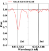 |
Fig. 2 Comparison of two neutral Zinc lines at λ = 4810.532 (left panel) and λ = 6362.338 (right panel)Å, for the same star (OGLE-GD-CEP-0228). The two spectral lines are highlighted with vertical dashed black lines, while the horizontal dashed black line defines the continuum (set at 1). |
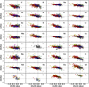 |
Fig. 3 Chemical elements in the form of [X/Fe] plotted against iron ([Fe/H]). Grey points represent stars already published in Ripepi et al. (2021); Trentin et al. (2023, 2024). Stars observed with UVES and published in Trentin et al. (2023, 2024) are coloured in yellow and red, respectively. New stars presented in this paper are coloured in blue, magenta, and green for PEPSI, HARPS, and UVES observations, respectively (see also the legend in 6). Vertical and horizontal dashed grey lines highlight the solar abundance position in the plot. |
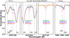 |
Fig. 4 Observed spectrum of RY Cru (solid black line, left and centre panel) and Gaia DR2 4644478166748030976 (solid orange line, right panel) in the region of DyII (5090.386 Å, left panel), ErII (5028.905 Å, centre panel) and LuII (6221.89 Å, right panel) spectral lines. The position of these and other visible lines is reported and highlighted with vertical dashed grey lines. Synthetic spectra computed for the best estimated abundance are reported in blue, while the same spectra with [X/H]=±0.5 dex are plotted in red and green, respectively. |
4.2 Radial gradients and spatial distribution
Following the same procedure as in Ripepi et al. (2021); Trentin et al. (2023, 2024), and described in Sect. 2, we calculated the Galactocentric distance (RGC) and the azimuthal angle of our targets and studied the radial gradients of all the measured chemical species (Fig. 5). The case of iron (usually used as a proxy of the metallicity) is shown (in their [X/H] form, Fig. 6). For all the chemical species, we carried out a linear regression using the Python LtsFit package (Cappellari et al. 2013), which implements a robust outliers removal, uses weights on both axes and estimates the error on the fitted parameters, together with the dispersion. The fitted slope for iron (−0.064 ±0.002 dex kpc−1) is in agreement with our latest results in Trentin et al. (2024), as well as most of the other chemical species. In more detail, light, α and iron-peak elements show a clear negative slope, with no precise trend as the atomic number increases. For neutron capture elements, they either have a shallower negative slope or gradients comparable with 0 (that is, no trend with RGC). The apparent change in the abundance trend previously highlighted for Sc, Cu, Y, Zn, and Zr in Trentin et al. (2024) is still present, but they now fall within the typical dispersion of the fit. In Fig. 7, we focus our attention on the polar and vertical distribution of our star. As was done in Trentin et al. (2024), we superimposed the spiral arm models from Reid et al. (2019). The upper right panel of figure 7 of Trentin et al. (2023) shows three stars (OGLE GD-CEP-0120, OGLE-GD CEP-0123, and OGLE GD-CEP-0214) displaced from the others, at RGC ≈18–19 kpc but |Z| < 500 pc. We verified from the light curves that these stars are DCEPs and investigated their galactocentric distances calculated from the distances reported in Bailer-Jones et al. (2021), and found a difference of around 4 kpc, and no significant difference in Z. With the new estimated RGC (≈14–15 kpc), these stars are now distributed more coherently with the others. These values are the ones reported in Table A.1 and used in this work. Three other stars, ATLAS J014.8936+45.4067, Gaia DR2 2246124001521354368, and V1253 Cen, caught our interest, since they are positioned at Z = −1.9, 3.0 (visible in the bottom right panel of Fig. 7), and 4.3 (top right panel of Fig. 7) kpc and distances from Bailer-Jones et al. (2021) agree with those estimated in our work within the errors. We studied the distribution of these objects in the energy-angular momentum diagram using Gaia proper motions and radial velocities and the Python package galpy (Bovy 2015)3. We found that these stars are located in the disc region of the diagram (i.e. see the bottom right panel of Figure 1 in Luongo et al. 2024), and further analysis is needed. Since the structure and identification of the spiral arms of the MW are still under debate, we used the Python SpiralMap package (Prusty & Khanna 2025) to discuss whether our targets can fit other models (see Levine et al. 2006; Hou & Han 2014; Drimmel et al. 2025, for detailed description of each of the models). Levine et al. (2006) proposed a logarithmic four-armed spiral model (ln(R/R0) = (ϕ(R) − ϕ0) tan ψ, with ψ the pitch angle and R0 and ϕ0 the Galactocentric distance and azimuth of the Sun, respectively) using a perturbed surface density map generated by the 21 cm hyperfine transition of neutral hydrogen. Three of these spirals, identified as the Carina, Local (or Orion), and Perseus arms, are plotted in the top left panel of Fig. 8. A bigger pitch angle (of the order of 20–25°) characterises these arms, compared to those used by Reid et al. (2019) (typically ≈10° and always <20°). It is evident that stars closer to the centre of the MW are tracing the Carina arm, while our outermost targets nicely fit the Perseus one.
Hou & Han (2014) proposed a polynomial-logarithmic model (ln(r) = a + b * θ + c * θ2 + d * θ3), using three different tracers (HII regions, Galactic molecular clouds, and methanol masers). In the top middle and top right panels of Fig. 8, two different models are shown, whether only HII regions or all three tracers are used, respectively. In this case, six different arms have been identified: Norma, Scutum-Centaurus, Sagittarius-Carina, Perseus, Outer and Outer+1 Arms (OSC), and the Local arm (not shown Fig. 8) that starts near the Perseus Arm, extends independently along the azimuth direction, and approaches the Carina Arm. The main difference with respect to the Levine et al. (2006) model is the azimuth-dependence of the pitch angles, which results in a smaller ‘aperture’ of the arms. Indeed, in this case, our furthermost stars either fit the Outer arm or both the Outer and the OSC arms, although in the latter case a slight change of the fitted parameters would be needed to have a better fit (as was done in Trentin et al. (2024) for Reid et al. (2019) models).
New models for the Perseus, Outer, and OSC arms were proposed by Sun et al. (2024), who analysed CO emission lines in more than 32 000 molecular clouds. These models, similar to what was done in Reid et al. (2019), allow the pitch angle to abruptly change at a certain angle, called a ‘kink’. Their model is shown in the bottom left panel of Fig. 8. In this case, only some of our furthest targets would trace the Outer arm (as in Reid et al. 2019), but no spiral arm would fit those at RGC > 15 kpc.
More recently, Drimmel et al. (2025) used new distances for almost 3000 Cepheids based on mid-IR WISE photometry (Skowron et al. 2025), and identified four spiral arms (Scutum, Sagittarius-Carina, Local, and Perseus) described with a logarithmic model and shown in the bottom middle panel of Fig. 8. Their models are in great agreement with those from Levine et al. (2006), and also in this case, our most distant stars better fit the Perseus arm.
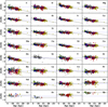 |
Fig. 5 Radial galactic gradients for each element in the form of [X/H]. Grey points represent stars already published in Ripepi et al. (2021); Trentin et al. (2023, 2024). Stars observed with UVES and published in Trentin et al. (2023, 2024) are coloured in yellow and red, respectively. New stars presented in this paper are coloured in blue, magenta, and green for PEPSI, HARPS, and UVES observations, respectively (see also the legend in 6). |
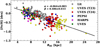 |
Fig. 6 Galactic iron radial gradient (in the form of [Fe/H] = α × RGC + β). The objects are colour-coded as in Fig. 3 and described in the legend. Grey points correspond to the DCEPs published in Ripepi et al. (2021) and Trentin et al. (2023) (except for those observed with UVES). The solid black line corresponds to the best-fitted line. Results of the fits are reported in both the figure and Table A.6. |
5 Discussion
In the first part of this section, we compare our estimation of the radial metallicity gradient with those found in the recent literature. When studying the radial metallicity gradient based on Cepheids, open clusters (OCs) are perfect targets for comparison. In most cases, information about the age is available, and it is possible to select clusters that are as young as Cepheids. In the fifth paper of the OCCAM project, Carbajo-Hijarrubia et al. (2024) collected a total of 36 OCs with metallicities estimated from high-resolution red clump spectra. They found a gradient of −0.059±0.017 dex kpc−1, in perfect agreement with ours. Moreover, they considered a second dataset (called OCCAM+) of 99 OCs composed of their sample complemented with OCs from the literature: Gaia-ESO Survey Data Release 5 (GES DR5, Magrini et al. 2023), Apache Point Observatory Galactic Evolution Experiment (APOGEE) DR17 (Myers et al. 2022), and Galactic Archaeology with HERMES (GALAH) DR3 (Spina et al. 2021). As in several other studies (Carrera et al. 2019; Donor et al. 2020; Zhang et al. 2021; Myers et al. 2022), they also detected a knee at around 11 kpc, over which the gradient flattens. In both cases of global slope (−0.062 ± 0.007 dex kpc−1) and inner slope (−0.069 ± 0.008 dex kpc−1), their results are in very good agreement with ours.
Yang et al. (2025) studied the abundance gradients of Mg, Si, Fe, and Ni using a homogeneous sample of 299 OCs. Their sample combined astrometric and photometric data from Hunt & Reffert (2023) (based on Gaia DR3) with metallicities from the Large Sky Area Multi-Object Fiber Spectroscopic Telescope (LAMOST) DR11 catalogue. These metallicities were determined using either the LAMOST Stellar Parameter pipeline (Luo et al. 2015) or the convolutional neural network (CNN) Stellar Parameter Convolutional Attention Network (SPCANet) (Wang et al. 2020). Although their slopes are systematically smaller (in terms of the absolute value), for the two iron-peak elements there is agreement at the 1.5σ and 1σ levels for Fe and Ni, respectively. It is worth mentioning that in both Carbajo-Hijarrubia et al. (2024) and Yang et al. (2025) it was found that the slope steepens with age, with the inner Galaxy young OCs showing lower [Fe/H] than old OCs, while in the outer Galaxy this trend reverses. For recent results regarding DCEPs, we refer the readers to the discussion in Trentin et al. (2024, 2023) and section 6 of Bono et al. (2024).
The rest of this section is dedicated to the comparison of recent literature estimates of Dy, Er, Lu, and Th with those estimated for DCEPs. In the context of the AMBRE project (de Laverny et al. 2013), whose main goals are to provide stellar parameters and abundances through automated algorithms of ESO archived spectra and to create chemical and kinematical maps of Galactic stellar populations, Dy was estimated for 5479 stars in Guiglion et al. (2018). The observations are based on UVES, HARPS, GIRAFFE (part of the FLAMES facility, Pasquini et al. 2002), and the Fiber-fed Extended Range Optical Spectrograph (FEROS) (Stahl et al. 1999) instruments. Through the study of [Eu/Ba], [Gd/Ba] and [Dy/Ba] as a function of metallicity (see their fig. 6), they found a clear indication of a different nucleosynthesis history in the thick disc between Eu and Gd–Dy. Measurements of Dy were carried out by Mishenina et al. (2022), based on 276 FGK dwarf stars in the galactic disc observed in Mishenina et al. (2013) with the 1.93-m telescope at the Observatoire de Haute-Provence (OHP) and the echelle-type spectrograph Echelle spectrograph for Observations of Diffuse Interstellar bands and Exoplanets (ELODIE, Baranne et al. 1996) and additional archival spectra collected with the Spectrographe pour l’Observation des Phénomènes des Intérieurs stellaires et des Exoplanètes (SOPHIE Perruchot et al. 2008). The trend of [Dy/Fe] against [Fe/H] for disc stars, shown in their Figure 5 (which includes data from Guiglion et al. 2018 and Spina et al. 2018), is in nice agreement with what is shown in Fig. 3, with [Dy/Fe] ranging from ≈0 and 1 dex for metallicities between −1 and 0 dex. Although for low metallicities (<−0.4 dex) our stars are typically more abundant in Dy ([Dy/Fe] between 0.5 and 1 dex) with respect to those presented in Mishenina et al. (2022), quantitative agreement is still found when comparing with data from Guiglion et al. (2018). The same is true for the other two ‘pure’ r-process elements analysed in this work, Eu and Gd.
In the context of the R-Process Alliance (RPA, Hansen et al. 2018), whose main objective is to investigate the r-process through the study of r-process-enriched stars, Hansen et al. (2025) observed the metal-poor star 2MASS J05383296–5904280 with the Space Telescope Imaging Spectrograph instrument mounted on the Hubble Space Telescope (HST/STIS Woodgate et al. 1998). The metallicity of this star is very low, −2.59 dex, while Er, Lu, and Th are enhanced with abundances of [Er/H] = −1.38, [Lu/H] = −1.26 dex, and [Th/H] = −1.18 dex (that is, [Er/Fe] = 1.21 dex, [Lu/Fe] = 1.33 dex, and [Th/Fe] = 1.41 dex). These results agree with the behaviour found in this paper of enhanced r-process abundances for lowmetallicity values. Dy, which was estimated as well ([Dy/H] = −1.24 dex, or equivalently [Dy/Fe] = 1.34 dex), is also enhanced and agrees with what was stated for the other elements. We point out that, as was already stated in Sect. 4, our measurements of Dy, Er, and Th are not definitive and their detection needs further attention.
Lyubimkov et al. (2022a) studied three red giant stars (EK Eri, OU And, and β Gem, with [Fe/H] = 0.1 dex, −0.11 dex and 0.03 dex, respectively) with strong magnetic fields using the NES echelle-spectrograph on the 6-m BTA telescope at the Special Astrophysical Observatory of the Russian Academy of Sciences. While these stars are thought to be descendants of magnetic Ap stars, no anomalies in the abundances of the heavy elements were found. In the case of erbium, for EK Eri and β Gem abundances of [Er/H] of 0.04 and 0.0 dex were estimated, but no Lu or Th was detected. These values, as well as their Dy estimation, are coherent with our measurements at solar metallicities. In a subsequent study (Lyubimkov et al. 2022b), nine K-Giants with planets were analysed and a similar estimation of Dy and Er was obtained. More recently, the sample of three magnetic red giants presented in Lyubimkov et al. (2022a) was complemented with twenty other objects (Lyubimkov et al. 2024), but in this case only Dy was measured.
Other recent literature estimations of either Er, Lu, or Th in very metal-poor stars are available in Saraf et al. (2023); Lin et al. (2025); da Silva & Smiljanic (2025) and references therein. These stars all have metallicities of <−2.0 dex, and are considered among the oldest objects in the Universe, making them a useful tool in studying the chemical enrichment of the MW and its past interaction with other systems. In these cases, all three elements are enhanced, following the other heavy neutron-capture elements. It is worth mentioning also the case of LAMOST J020623.21+494127.9, analysed in Xie et al. (2024) and Ashraf et al. (2025). This star, although not very metal-poor (with a metallicity of [Fe/H] = −0.54 dex), is still an r-process-enhanced object (see table 2 in Xie et al. 2024) with a reported lutetium abundance of 0.20 dex.
The only estimation of these three elements for Cepheids was reported for the first time in Kovtyukh et al. (2023) ([Er/H] = +1.03 dex, [Lu/H] = +0.4 dex, and [Th/H] = +0.98 dex) for a DCEP in our sample (OGLE GD-CEP-1353, reported in this work as ASASSN-V J074354.86-323013.7), but not all the abundances match within the errors, probably due to the different code used by the authors (see their Section 2).
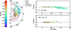 |
Fig. 7 Left panel: galactic polar distribution of the stars for azimuthal angle between −90 and 90 degrees. Circles with black borders highlight the targets presented in this work. All stars are colour-coded according to the measured iron abundance. The position of the sun is shown with a yellow-black symbol. Spiral arms adapted from Reid et al. (2019) are shown in different colours (see legend). Right panel: cartesian representation of the height above or below the galactic plane as a function of RGC in two opposite directions with respect to the Galactic centre-Sun line (top and bottom panels, respectively). The colour coding and the symbols are as in the left panel. The grey area delimits the region at |Z| < 300 pc. |
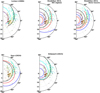 |
Fig. 8 Spiral arm models from Levine et al. (2006) (HI regions), Hou & Han (2014) (using only HII regions or three different tracers), Sun et al. (2024) (CO regions), and Drimmel et al. (2025) (DCEPs) are superimposed on our targets in the top left, top middle, top right, bottom left and bottom middle panels, respectively. All the models (with the exception of Sun et al. 2024) are collected in the Python SpiralMap package (Prusty & Khanna 2025). Spiral arm colours are the same as those in Fig. 7. |
6 Summary
In this eighth work in the context of the C-MetaLL project, we collected and analysed a total of 136 spectra, corresponding to 60 DCEPs, 7 of which are repeated targets already published in previous C-MetaLL works, and 2 are SMC stars. One of the main characteristics of this dataset is that more than half of the objects are long-period Cepheids, with pulsational periods ranging from 15 to 70 days. Spectra were obtained with UVES@VLT, HARPS-N@TNG, and PEPSI@LBT. For each target, radial velocity, effective temperature, surface gravity, micro- and macro-turbulence velocities, and LTE chemical abundances were obtained. Following the instruction from Amarsi et al. (2020), we applied a correction of 0.1 dex on our Na abundances to take into consideration non-LTE effects, while for the other elements, corrections were neglected. We confirm the low-metallicity nature of the SMC stars. We complemented our galactic sample with previously published targets in the context of the C-MetaLL project, for a final sample of 340 different stars (289 from past papers and 51 from present work, respectively). Using an updated list of trusted spectral lines, we revisited the abundances for all the stars for those elements with new available lines. While for most elements, such as O, C, V, Ti, Ba, and Nd, no statistical or systematic difference was detected between the previously estimated abundances and the new ones, the abundances of other chemical species (Sc, Cu, Zn, Y, and Zr) changed by more than 0.1 dex, especially in the low-metallicity regimee in which the available spectral lines are usually weaker and more affected by noise. The revisited abundances for these elements show a less pronounced or absent ‘jump’ in the radial direction. Up to 33 chemical species have been detected, with Dy estimated for the first time in DCEPs and 3 elements (Er, Lu, and Th) estimated for several objects (see Kovtyukh et al. 2023, for the first detection of these elements in Cepheids). For all the elements we studied both their trends with respect to the iron content and their galactocentric radial gradients. In more detail:
For light elements, we found a decreasing trend with increasing metallicity, with [C/Fe] and [O/Fe] reaching sub-solar values and [Al/Fe] reaching solar values at higher [Fe/H]. Sodium instead is constant along the whole metallicity range, at [Na/Fe]≈0.4 dex;
α and iron peak elements show a decreasing behaviour followed by a flattening trend. Exceptions are given by: [Mn/Fe] and [Zn/Fe], which are relatively constant over the whole range; [Cu/Fe], with first a flattening trend and then a decrease at higher metallicities; and [Sc/Fe], which instead shows a slight enhancement for metal-rich stars;
Neutron-capture elements, including the newly detected elements, show either an arch-form or a descending trend. Previously missing Ce, Sm, Eu, and Gd abundances from published DCEPs in the C-MetaLL project have now been estimated for several stars. The detected Dy line at λ = 5090.386 Å mostly appears as a deformation of the wing of a close Fe I at λ = 5090.773 Å, but the effect is in some cases sensible enough to estimate this element. Er was estimated thanks to a weak line at λ = 5028.905 Å, while Lu for most stars presents a clear and isolated line at λ = 6221.891 Å;
We confirm a clear negative galactocentric radial gradient for most of our elements. Heavy neutron capture elements show instead shallower or null gradients, with [X/H] abundances mostly constant over a broad range of distances (5–20 kpc). The iron metallicity gradient −0.064 ± 0.002 dex kpc−1 is in good agreement with our previous work and recent literature gradients found for young OCs;
We studied the polar distribution of our stars in the MW disc, comparing different spiral arms models (Levine et al. 2006; Hou & Han 2014; Reid et al. 2019; Sun et al. 2024; Drimmel et al. 2025). Depending on which tracer and/or analytic function was used, different results were obtained. In this context, while the stars closest to the galactic centre nicely trace the Sgr-Car arm for all the models, those between 10 and 20 kpc can either trace the Perseus arm (Levine et al. 2006; Drimmel et al. 2025), the Norma-Outer arm (Hou & Han 2014; Sun et al. 2024) or both the Outer and the OSC arms (Hou & Han 2014; Reid et al. 2019).
It is important to stress that, beyond their importance in the study of the metallicity dependence of the DCEPs PL relations, the main focus of the C-MetaLL project, this work highlights how Galactic DCEPs can prove themselves as important tiles in tracing the young population of spiral arms and can be essential in the analysis of chemical evolution of the galactic disc. Most measurements of the heaviest elements are usually made for chemically peculiar main-sequence A and B stars, red giants with strong magnetic fields, probable descendants of Ap stars, and very metal-poor old stars ([Fe/H]<−2 dex). The detection of chemical species such as Er and Lu in young and relatively metal-rich stars such as DCEPs can constitute a turning point in the study of galactic enrichment, as well as offering a new scenario for investigating the production channel of neutron-capture elements and the differences between slow and rapid processes. However, it should be emphasised that, unlike in chemically peculiar main-sequence stars, where the large overabundances of heavy and rare-earth elements originate from atmospheric diffusion effects, the abundances measured in Cepheids genuinely reflect the chemical composition of the interstellar medium from which they formed, and thus provide reliable tracers of the Galactic chemical evolution.
Data availability
Full Tables A.1–A.4 are available at the CDS via https://cdsarc.cds.unistra.fr/viz-bin/cat/J/A+A/707/A142.
Acknowledgements
Based on observations European Southern Observatory programs P105.20MX.001; P106.2129.001; 108.227Z; 109.231T; 110.23WM; 112.25NA, on the Telescopio Nazionale Galileo programmes A39TAC_9; A40TAC_11; A41TAC_29; A42TAC_15; A43TAC_16; A44TAC_27; A45TAC_12; A46TAC_15; A47TAC_18. Based on observations obtained at the Canada-France-Hawaii Telescope (CFHT) which is operated by the National Research Council of Canada, the Institut National des Sciences de l´Univers of the Centre National de la Recherche Scientique of France, and the University of Hawaii. Based on observations obtained at the Large Binocular Telescope programs IT-2019B-014 and IT-2021-2022-24). This research has made use of the SIMBAD database operated at CDS, Strasbourg, France. We acknowledge funding from INAF GO-GTO grant 2023 “C-MetaLL - Cepheid metallicity in the Leavitt law” (PI: V. Ripepi). We acknowledge support from Project PRIN MUR 2022 (code 2022ARWP9C) “Early Formation and Evolution of Bulge and HalO (EFEBHO)” (PI: M. Marconi), funded by European Union - Next Generation EU; INAF Large grant 2023 MOVIE (PI: M. Marconi). This work has made use of data from the European Space Agency (ESA) mission Gaia (https://www.cosmos.esa.int/gaia), processed by the Gaia Data Processing and Analysis Consortium (DPAC, https://www.cosmos.esa.int/web/gaia/dpac/consortium). Funding for the DPAC has been provided by national institutions, in particular, the institutions participating in the Gaia Multilateral Agreement. This research was supported by the Munich Institute for Astro-, Particle and BioPhysics (MIAPbP), which is funded by the Deutsche Forschungsgemeinschaft (DFG, German Research Foundation) under Germany´s Excellence Strategy – EXC-2094 – 390783311. This research was supported by the International Space Science Institute (ISSI) in Bern/Beijing through ISSI/ISSI-BJ International Team project ID #24-603 - “EXPANDING Universe” (EXploiting Precision AstroNomical Distance INdicators in the Gaia Universe). A.B. thanks the funding from the Anusandhan National Research Foundation (ANRF) under the Prime Minister Early Career Research Grant scheme (ANRF/ECRG/2024/000675/PMS).
References
- Amarsi, A. M., Lind, K., Osorio, Y., et al. 2020, A&A, 642, A62 [EDP Sciences] [Google Scholar]
- Anand, G. S., Tully, R. B., Cohen, Y., et al. 2025, ApJ, 982, 26 [Google Scholar]
- Ashraf, M. Z., Cui, W., & Li, H. 2025, Res. Astron. Astrophys., 25, 085015 [Google Scholar]
- Asplund, M., Amarsi, A. M., & Grevesse, N. 2021, A&A, 653, A141 [NASA ADS] [CrossRef] [EDP Sciences] [Google Scholar]
- Bailer-Jones, C. A. L., Rybizki, J., Fouesneau, M., Demleitner, M., & Andrae, R. 2021, AJ, 161, 147 [Google Scholar]
- Baranne, A., Queloz, D., Mayor, M., et al. 1996, A&AS, 119, 373 [Google Scholar]
- Bhardwaj, A., Riess, A. G., Catanzaro, G., et al. 2023, ApJ, 955, L13 [NASA ADS] [CrossRef] [Google Scholar]
- Bhardwaj, A., Ripepi, V., Testa, V., et al. 2024, A&A, 683, A234 [NASA ADS] [CrossRef] [EDP Sciences] [Google Scholar]
- Bhardwaj, A., Matsunaga, N., Huang, C. D., Riess, A. G., & Rejkuba, M. 2025, ApJ, 990, 63 [Google Scholar]
- Bono, G., Braga, V. F., & Pietrinferni, A. 2024, A&A Rev., 32, 4 [Google Scholar]
- Bovy, J. 2015, ApJS, 216, 29 [NASA ADS] [CrossRef] [Google Scholar]
- Brauer, K., Ji, A. P., Drout, M. R., & Frebel, A. 2021, ApJ, 915, 81 [NASA ADS] [CrossRef] [Google Scholar]
- Breuval, L., Riess, A. G., Casertano, S., et al. 2024, ApJ, 973, 30 [Google Scholar]
- Breuval, L., Anand, G. S., Anderson, R. I., et al. 2025, ApJ, 994, 111 [Google Scholar]
- Cameron, A. G. W. 2003, ApJ, 587, 327 [NASA ADS] [CrossRef] [Google Scholar]
- Cappellari, M., Scott, N., Alatalo, K., et al. 2013, MNRAS, 432, 1709 [Google Scholar]
- Carbajo-Hijarrubia, J., Casamiquela, L., Carrera, R., et al. 2024, A&A, 687, A239 [NASA ADS] [CrossRef] [EDP Sciences] [Google Scholar]
- Carrera, R., Bragaglia, A., Cantat-Gaudin, T., et al. 2019, A&A, 623, A80 [NASA ADS] [CrossRef] [EDP Sciences] [Google Scholar]
- Castelli, F., & Hubrig, S. 2004, A&A, 425, 263 [NASA ADS] [CrossRef] [EDP Sciences] [Google Scholar]
- Cosentino, R., Lovis, C., Pepe, F., et al. 2012, SPIE Conf. Ser., 8446, 84461V [Google Scholar]
- Cowan, J. J., Sneden, C., Lawler, J. E., et al. 2021, Rev. Mod. Phys., 93, 015002 [Google Scholar]
- Cowley, C. R., & Greenberg, M. 1987, PASP, 99, 1201 [Google Scholar]
- da Silva, A. R., & Smiljanic, R. 2025, A&A, 696, A122 [NASA ADS] [CrossRef] [EDP Sciences] [Google Scholar]
- da Silva, R., D’Orazi, V., Palla, M., et al. 2023, A&A, 678, A195 [NASA ADS] [CrossRef] [EDP Sciences] [Google Scholar]
- de Laverny, P., Recio-Blanco, A., Worley, C. C., et al. 2013, The Messenger, 153, 18 [NASA ADS] [Google Scholar]
- De Somma, G., Marconi, M., Ripepi, V., et al. 2025, ApJ, 984, L60 [Google Scholar]
- Dekker, H., D’Odorico, S., Kaufer, A., Delabre, B., & Kotzlowski, H. 2000, SPIE Conf. Ser., 4008, 534 [Google Scholar]
- Donor, J., Frinchaboy, P. M., Cunha, K., et al. 2020, AJ, 159, 199 [NASA ADS] [CrossRef] [Google Scholar]
- Drimmel, R., Khanna, S., Poggio, E., & Skowron, D. M. 2025, A&A, 698, A230 [NASA ADS] [CrossRef] [EDP Sciences] [Google Scholar]
- Fernández, R., Foucart, F., & Lippuner, J. 2020, MNRAS, 497, 3221 [CrossRef] [Google Scholar]
- Gaia Collaboration (Drimmel, R., et al.) 2023a, A&A, 674, A37 [CrossRef] [EDP Sciences] [Google Scholar]
- Gaia Collaboration (Vallenari, A., et al.) 2023b, A&A, 674, A1 [NASA ADS] [CrossRef] [EDP Sciences] [Google Scholar]
- Genovali, K., Lemasle, B., Bono, G., et al. 2014, A&A, 566, A37 [NASA ADS] [CrossRef] [EDP Sciences] [Google Scholar]
- Gravity Collaboration (Abuter, R., et al.) 2022, A&A, 657, L12 [NASA ADS] [CrossRef] [Google Scholar]
- Gray, D. F., & Johanson, H. L. 1991, PASP, 103, 439 [NASA ADS] [CrossRef] [Google Scholar]
- Guiglion, G., de Laverny, P., Recio-Blanco, A., & Prantzos, N. 2018, A&A, 619, A143 [NASA ADS] [CrossRef] [EDP Sciences] [Google Scholar]
- Hansen, T. T., Holmbeck, E. M., Beers, T. C., et al. 2018, ApJ, 858, 92 [Google Scholar]
- Hansen, T. T., Roederer, I. U., Shah, S. P., et al. 2025, A&A, 697, A127 [NASA ADS] [CrossRef] [EDP Sciences] [Google Scholar]
- Hou, L. G., & Han, J. L. 2014, A&A, 569, A125 [NASA ADS] [CrossRef] [EDP Sciences] [Google Scholar]
- Hoyt, T. J., Jang, I. S., Freedman, W. L., et al. 2025, arXiv e-prints [arXiv:2503.11769] [Google Scholar]
- Hunt, E. L., & Reffert, S. 2023, A&A, 673, A114 [NASA ADS] [CrossRef] [EDP Sciences] [Google Scholar]
- Kobayashi, C., Karakas, A. I., & Lugaro, M. 2020, ApJ, 900, 179 [Google Scholar]
- Kovtyukh, V., & Gorlova, N. 2000, A&A, 358, 587 [NASA ADS] [Google Scholar]
- Kovtyukh, V., Lemasle, B., Bono, G., et al. 2022, MNRAS, 510, 1894 [Google Scholar]
- Kovtyukh, V. V., Andrievsky, S. M., Werner, K., & Korotin, S. A. 2023, A&A, 679, A140 [NASA ADS] [CrossRef] [EDP Sciences] [Google Scholar]
- Kurucz, R. L. 1993, IAU Colloq., 138, 87 [NASA ADS] [Google Scholar]
- Kurucz, R. 1995, Atomic Line List (Cambridge, MA: Smithsonian Astrophysical Observatory) [Google Scholar]
- Kurucz, R. L., & Avrett, E. H. 1981, SAO Special Report, 391 [Google Scholar]
- Lawler, J. E., Sneden, C., Cowan, J. J., et al. 2008, ApJS, 178, 71 [Google Scholar]
- Leavitt, H. S., & Pickering, E. C. 1912, Harvard College Observ. Circ., 173, 1 [NASA ADS] [Google Scholar]
- Lee, A. J., Freedman, W. L., Madore, B. F., et al. 2025, ApJ, 985, 182 [Google Scholar]
- Lemasle, B., Hajdu, G., Kovtyukh, V., et al. 2018, A&A, 618, A160 [NASA ADS] [CrossRef] [EDP Sciences] [Google Scholar]
- Lemasle, B., Lala, H. N., Kovtyukh, V., et al. 2022, A&A, 668, A40 [NASA ADS] [CrossRef] [EDP Sciences] [Google Scholar]
- Leone, F., & Catanzaro, G. 2004, A&A, 425, 271 [NASA ADS] [CrossRef] [EDP Sciences] [Google Scholar]
- Levine, E. S., Blitz, L., & Heiles, C. 2006, Science, 312, 1773 [NASA ADS] [CrossRef] [Google Scholar]
- Li, S., Riess, A. G., Scolnic, D., Casertano, S., & Anand, G. S. 2025, ApJ, 988, 97 [Google Scholar]
- Lin, Y., Li, H., Jiang, R., et al. 2025, ApJ, 984, L43 [Google Scholar]
- Luck, R. E. 2018, AJ, 156, 171 [Google Scholar]
- Luck, R. E., & Lambert, D. L. 2011, AJ, 142, 136 [Google Scholar]
- Luo, A. L., Zhao, Y.-H., Zhao, G., et al. 2015, Res. Astron. Astrophys., 15, 1095 [Google Scholar]
- Luongo, E., Ripepi, V., Marconi, M., et al. 2024, A&A, 690, L17 [NASA ADS] [CrossRef] [EDP Sciences] [Google Scholar]
- Lyubimkov, L. S., Korotin, S. A., Petrov, D. V., et al. 2022a, Astrophysics, 65, 53 [Google Scholar]
- Lyubimkov, L. S., Poklad, D. B., & Korotin, S. A. 2022b, Astrophysics, 65, 494 [Google Scholar]
- Lyubimkov, L. S., Korotin, S. A., Petrov, D. V., & Poklad, D. B. 2024, MNRAS, 528, 304 [Google Scholar]
- Madore, B. F. 1982, ApJ, 253, 575 [NASA ADS] [CrossRef] [Google Scholar]
- Madore, B. F., & Freedman, W. L. 2025, ApJ, 983, 161 [Google Scholar]
- Magrini, L., Viscasillas Vázquez, C., Spina, L., et al. 2023, A&A, 669, A119 [NASA ADS] [CrossRef] [EDP Sciences] [Google Scholar]
- Matsunaga, N., Taniguchi, D., Elgueta, S. S., et al. 2023, ApJ, 954, 198 [NASA ADS] [CrossRef] [Google Scholar]
- Mayor, M., Pepe, F., Queloz, D., et al. 2003, The Messenger, 114, 20 [NASA ADS] [Google Scholar]
- Minniti, J. H., Sbordone, L., Rojas-Arriagada, A., et al. 2020, A&A, 640, A92 [EDP Sciences] [Google Scholar]
- Mishenina, T. V., Pignatari, M., Korotin, S. A., et al. 2013, A&A, 552, A128 [NASA ADS] [CrossRef] [EDP Sciences] [Google Scholar]
- Mishenina, T., Pignatari, M., Gorbaneva, T., et al. 2022, MNRAS, 516, 3786 [NASA ADS] [CrossRef] [Google Scholar]
- Myers, N., Donor, J., Spoo, T., et al. 2022, AJ, 164, 85 [NASA ADS] [CrossRef] [Google Scholar]
- Nelder, J. A., & Mead, R. 1965, Comp. J., 7, 308 [CrossRef] [Google Scholar]
- Pasquini, L., Avila, G., Blecha, A., et al. 2002, The Messenger, 110, 1 [Google Scholar]
- Perruchot, S., Kohler, D., Bouchy, F., et al. 2008, SPIE Conf. Ser., 7014, 70140J [Google Scholar]
- Pietrukowicz, P., Soszyński, I., & Udalski, A. 2021, Acta Astron., 71, 205 [NASA ADS] [Google Scholar]
- Planck Collaboration VI. 2020, A&A, 641, A6 [NASA ADS] [CrossRef] [EDP Sciences] [Google Scholar]
- Prusty, A. K., & Khanna, S. 2025, arXiv e-prints [arXiv:2506.11383] [Google Scholar]
- Ralchenko, A. K., & Reader, J. 2019, National Institute of Standards and Technology, Gaithersburg, MD https://doi.org/10.18434/T4W30F [Google Scholar]
- Reid, M. J., Menten, K. M., Brunthaler, A., et al. 2019, ApJ, 885, 131 [Google Scholar]
- Riess, A. G., Casertano, S., Yuan, W., et al. 2021, ApJ, 908, L6 [NASA ADS] [CrossRef] [Google Scholar]
- Riess, A. G., Yuan, W., Macri, L. M., et al. 2022, ApJ, 934, L7 [NASA ADS] [CrossRef] [Google Scholar]
- Ripepi, V., Molinaro, R., Musella, I., et al. 2019, A&A, 625, A14 [NASA ADS] [CrossRef] [EDP Sciences] [Google Scholar]
- Ripepi, V., Catanzaro, G., Molinaro, R., et al. 2021, MNRAS, 508, 4047 [NASA ADS] [CrossRef] [Google Scholar]
- Ripepi, V., Catanzaro, G., Clementini, G., et al. 2022, A&A, 659, A167 [NASA ADS] [CrossRef] [EDP Sciences] [Google Scholar]
- Ripepi, V., Clementini, G., Molinaro, R., et al. 2023, A&A, 674, A17 [NASA ADS] [CrossRef] [EDP Sciences] [Google Scholar]
- Romaniello, M., Primas, F., Mottini, M., et al. 2008, A&A, 488, 731 [NASA ADS] [CrossRef] [EDP Sciences] [Google Scholar]
- Romaniello, M., Riess, A., Mancino, S., et al. 2022, A&A, 658, A29 [NASA ADS] [CrossRef] [EDP Sciences] [Google Scholar]
- Rosswog, S., Sollerman, J., Feindt, U., et al. 2018, A&A, 615, A132 [NASA ADS] [CrossRef] [EDP Sciences] [Google Scholar]
- Saraf, P., Allende Prieto, C., Sivarani, T., et al. 2023, MNRAS, 524, 5607 [NASA ADS] [CrossRef] [Google Scholar]
- Skowron, D. M., Skowron, J., Mróz, P., et al. 2019, Science, 365, 478 [Google Scholar]
- Skowron, D. M., Drimmel, R., Khanna, S., et al. 2025, ApJS, 278, 57 [Google Scholar]
- Sneden, C., Cowan, J. J., & Gallino, R. 2008, ARA&A, 46, 241 [Google Scholar]
- Spina, L., Meléndez, J., Karakas, A. I., et al. 2018, MNRAS, 474, 2580 [NASA ADS] [Google Scholar]
- Spina, L., Ting, Y.-S., De Silva, G. M., et al. 2021, MNRAS, 503, 3279 [CrossRef] [Google Scholar]
- Stahl, O., Kaufer, A., & Tubbesing, S. 1999, ASP Conf. Ser., 188, 331 [NASA ADS] [Google Scholar]
- Strassmeier, K. G., Ilyin, I., Järvinen, A., et al. 2015, Astron. Nachr., 336, 324 [NASA ADS] [CrossRef] [Google Scholar]
- Strassmeier, K. G., Ilyin, I., & Steffen, M. 2018, A&A, 612, A44 [NASA ADS] [CrossRef] [EDP Sciences] [Google Scholar]
- Sun, Y., Yang, J., Zhang, S., et al. 2024, ApJ, 977, L35 [Google Scholar]
- Trentin, E., Ripepi, V., Catanzaro, G., et al. 2023, MNRAS, 519, 2331 [Google Scholar]
- Trentin, E., Catanzaro, G., Ripepi, V., et al. 2024, A&A, 690, A246 [NASA ADS] [CrossRef] [EDP Sciences] [Google Scholar]
- Wang, R., Luo, A. L., Chen, J.-J., et al. 2020, ApJ, 891, 23 [Google Scholar]
- Woodgate, B. E., Kimble, R. A., Bowers, C. W., et al. 1998, PASP, 110, 1183 [NASA ADS] [CrossRef] [Google Scholar]
- Woosley, S. E., Wilson, J. R., Mathews, G. J., Hoffman, R. D., & Meyer, B. S. 1994, ApJ, 433, 229 [Google Scholar]
- Xie, X.-J., Shi, J., Yan, H.-L., et al. 2024, ApJ, 970, L30 [NASA ADS] [CrossRef] [Google Scholar]
- Yang, G., Zhao, J., Yang, Y., et al. 2025, AJ, 169, 214 [Google Scholar]
- Zhang, H., Chen, Y., & Zhao, G. 2021, ApJ, 919, 52 [NASA ADS] [CrossRef] [Google Scholar]
Appendix A Tables
Main properties of the 59 programme DCEPs
Observation information and atmospheric parameters for the 136 spectra analysed in this work.
List of observed spectral lines in our spectra.
Estimated chemical abundances for the whole C-MetaLL dataset of 340 stars.
Estimated chemical abundances for the SMC DCEPs Gaia DR2 4638315266636230400 and Gaia DR2 4644478166748030976.
Results of the fitting.
All Tables
Observation information and atmospheric parameters for the 136 spectra analysed in this work.
Estimated chemical abundances for the SMC DCEPs Gaia DR2 4638315266636230400 and Gaia DR2 4644478166748030976.
All Figures
|
Fig. 1 Distribution of the C-MetaLL sample along the Galactic disc. The points are colour-coded according to the pulsator’s period. Targets presented in this work are highlighted with black borders. The position of the sun is shown with a yellow-black circle. |
| In the text | |
|
Fig. 2 Comparison of two neutral Zinc lines at λ = 4810.532 (left panel) and λ = 6362.338 (right panel)Å, for the same star (OGLE-GD-CEP-0228). The two spectral lines are highlighted with vertical dashed black lines, while the horizontal dashed black line defines the continuum (set at 1). |
| In the text | |
|
Fig. 3 Chemical elements in the form of [X/Fe] plotted against iron ([Fe/H]). Grey points represent stars already published in Ripepi et al. (2021); Trentin et al. (2023, 2024). Stars observed with UVES and published in Trentin et al. (2023, 2024) are coloured in yellow and red, respectively. New stars presented in this paper are coloured in blue, magenta, and green for PEPSI, HARPS, and UVES observations, respectively (see also the legend in 6). Vertical and horizontal dashed grey lines highlight the solar abundance position in the plot. |
| In the text | |
|
Fig. 4 Observed spectrum of RY Cru (solid black line, left and centre panel) and Gaia DR2 4644478166748030976 (solid orange line, right panel) in the region of DyII (5090.386 Å, left panel), ErII (5028.905 Å, centre panel) and LuII (6221.89 Å, right panel) spectral lines. The position of these and other visible lines is reported and highlighted with vertical dashed grey lines. Synthetic spectra computed for the best estimated abundance are reported in blue, while the same spectra with [X/H]=±0.5 dex are plotted in red and green, respectively. |
| In the text | |
|
Fig. 5 Radial galactic gradients for each element in the form of [X/H]. Grey points represent stars already published in Ripepi et al. (2021); Trentin et al. (2023, 2024). Stars observed with UVES and published in Trentin et al. (2023, 2024) are coloured in yellow and red, respectively. New stars presented in this paper are coloured in blue, magenta, and green for PEPSI, HARPS, and UVES observations, respectively (see also the legend in 6). |
| In the text | |
|
Fig. 6 Galactic iron radial gradient (in the form of [Fe/H] = α × RGC + β). The objects are colour-coded as in Fig. 3 and described in the legend. Grey points correspond to the DCEPs published in Ripepi et al. (2021) and Trentin et al. (2023) (except for those observed with UVES). The solid black line corresponds to the best-fitted line. Results of the fits are reported in both the figure and Table A.6. |
| In the text | |
|
Fig. 7 Left panel: galactic polar distribution of the stars for azimuthal angle between −90 and 90 degrees. Circles with black borders highlight the targets presented in this work. All stars are colour-coded according to the measured iron abundance. The position of the sun is shown with a yellow-black symbol. Spiral arms adapted from Reid et al. (2019) are shown in different colours (see legend). Right panel: cartesian representation of the height above or below the galactic plane as a function of RGC in two opposite directions with respect to the Galactic centre-Sun line (top and bottom panels, respectively). The colour coding and the symbols are as in the left panel. The grey area delimits the region at |Z| < 300 pc. |
| In the text | |
|
Fig. 8 Spiral arm models from Levine et al. (2006) (HI regions), Hou & Han (2014) (using only HII regions or three different tracers), Sun et al. (2024) (CO regions), and Drimmel et al. (2025) (DCEPs) are superimposed on our targets in the top left, top middle, top right, bottom left and bottom middle panels, respectively. All the models (with the exception of Sun et al. 2024) are collected in the Python SpiralMap package (Prusty & Khanna 2025). Spiral arm colours are the same as those in Fig. 7. |
| In the text | |
Current usage metrics show cumulative count of Article Views (full-text article views including HTML views, PDF and ePub downloads, according to the available data) and Abstracts Views on Vision4Press platform.
Data correspond to usage on the plateform after 2015. The current usage metrics is available 48-96 hours after online publication and is updated daily on week days.
Initial download of the metrics may take a while.