© The Authors 2026

1. Introduction

Understanding the internal dynamics of evolved solar-like stars remains one of the major challenges in asteroseismology. Internal dynamical processes can be probed using oscillations that consist of acoustic pressure modes (p modes) and buoyancy-driven gravity modes (g modes). In evolved solar-like stars, p and g modes can couple across their respective cavities, giving rise to mixed modes (e.g. Unno et al. 1989; Takata 2016a), first detected by Beck et al. (2011). Mixed-mode analyses have revealed the core and the envelope rotation rates of sub-giant and red giant stars (e.g. Beck et al. 2011; Deheuvels et al. 2012; Mosser et al. 2012a; Deheuvels et al. 2014; Di Mauro et al. 2016; Gehan et al. 2018; Li et al. 2024). However, measured rotational gradients are substantially weaker than those predicted by hydrodynamical theoretical models of angular momentum evolution (e.g. Eggenberger et al. 2012; Marques et al. 2013; Ceillier et al. 2013; Eggenberger et al. 2017, 2019). This discrepancy indicates the presence of missing angular momentum transport mechanisms in our representation of angular momentum transport in stars. Several processes have been proposed to enhance transport, including meridional circulation (Zahn 1992; Maeder & Zahn 1998; Mathis & Zahn 2004; Decressin et al. 2009), hydrodynamical instabilities (Zahn 1992), mixed modes (Belkacem et al. 2015; Bordadágua et al. 2025), internal gravity waves (Schatzman 1993; Fuller et al. 2014; Pinçon et al. 2017; Rogers & Ratnasingam 2025), and magnetic processes such as transport by Alfvén waves and magnetic tension (e.g. Mestel & Weiss 1987; Zahn et al. 2007; Takahashi & Langer 2021; Gouhier et al. 2022), magneto-rotational instabilities (Meduri et al. 2024), magnetic webs (Skoutnev & Beloborodov 2025a), or transport by the Tayler-Spruit dynamo (e.g. Tayler 1973; Spruit 2002; Fuller et al. 2019; Moyano et al. 2023; Skoutnev & Beloborodov 2025b). To date, no observational constraints have unequivocally identified any overarching dominant physical mechanism responsible for angular momentum transport along stellar evolution.

To better constrain the efficiency of such newly proposed angular momentum transport mechanisms, more refined seismic diagnostics are required. So far, most efforts to constrain stellar internal rotation rates have focused on dipolar mixed modes, i.e. modes with degree ℓ = 1. Extending the analysis beyond dipole (ℓ = 1) modes to include quadrupole mixed modes (ℓ = 2) offers the prospect of significantly strengthening and adding constraints on internal dynamics. This extension not only increases the number of available observational probes but also provides sensitivity to different dynamical kernels, as modes of different degrees sample distinct regions of the stellar interior, particularly within the convective zone (Hekker & Christensen-Dalsgaard 2017). The probing power of ℓ = 2 mixed modes and our ability to use them are limited by two major factors: (i) The p- and g-mode cavities sit further away from each other than those of ℓ = 1 modes, leading to an expected much weaker coupling strength that reduces the height of the ℓ = 2 mixed modes in the power spectral density (hereafter PSD, Dupret et al. 2009; Grosjean et al. 2014; Mosser et al. 2018). (ii) The presence of near-degeneracy effects between adjacent multiplets distort the splitting structure (Lynden-Bell & Ostriker 1967; Dziembowski & Goode 1992; Deheuvels et al. 2012, 2014, 2017; Mosser et al. 2018; Ong et al. 2022; Li et al. 2024; Ahlborn et al. 2025) and prevent straightforward identification and interpretation of the ℓ = 2 mixed-mode frequency pattern.

While the above-mentioned point (i) is a detectability limit, point (ii) reduces our ability to identify modes. Standard first-order perturbation theory predicts symmetric splittings in slowly-rotating stars (e.g. Aerts et al. 2010; Goupil et al. 2013; Deheuvels et al. 2014; Gehan et al. 2018). However, if two unperturbed modes are close in frequency, their eigenfunctions are no longer independent. The resulting near-degeneracy introduces off-diagonal interaction terms in the oscillation equations, producing an observable asymmetry in the mixed-mode frequency pattern (Lynden-Bell & Ostriker 1967; Dziembowski & Goode 1992; Deheuvels et al. 2017; Mosser et al. 2018; Ong et al. 2022; Li et al. 2024; Ahlborn et al. 2025). Despite several studies investigating near-degeneracy effects on oscillation frequencies (e.g. Deheuvels et al. 2017; Mosser et al. 2018; Ong et al. 2022; Li et al. 2024; Ahlborn et al. 2025) and efforts to include ℓ = 2 modes in seismic analysis (Deheuvels et al. 2012, 2014, 2017; Benomar et al. 2013), no asymptotic framework has been developed yet to explicitly compute the near-degeneracy interaction terms in the mixed-mode basis. For instance, Li et al. (2024) performed an implicit treatment of these effects, while Ong et al. (2022) carried out the calculation in the π–γ decoupled mode basis. In this work, we present a new asymptotic formalism for mixed quadrupole modes that explicitly incorporates near-degeneracy effects through non-diagonal near-degeneracy terms in the mixed-mode basis. This approach enables us to compute the near-degeneracy terms directly in the asymptotic limit and solve the associated quadratic eigenvalue problem. It also offers two main advantages: (i) It preserves the mixed-mode basis, which simplifies the implementation for direct use in data analysis, similar to the method extensively used to analyse ℓ = 1 mixed modes. (ii) It provides explicit asymptotic estimates of the off-diagonal near-degeneracy terms, allowing for closed-form near-degeneracy corrections derived from quantum perturbation theory.

This article is structured as follows: In Section 2 we lay the theoretical basis for this work and show the development leading to the asymptotic expression of the off-diagonal near-degeneracy terms. In Section 3, we introduce the global Bayesian framework and the priors we used for simultaneously fitting of our radial and ℓ = 1, 2 mixed modes. Finally, in Section 4 we describe how we applied our new formalism and analysis pipeline to two early red giant stars observed by the NASA Kepler mission (Borucki et al. 2010). We started with KIC 7341231, which has already been characterised with numerical methods by Deheuvels et al. (2017), to demonstrate the robustness of our prescription. We then performed the global fit of mixed modes in the new candidate, KIC 8179973, which shows strong near-degeneracy effects in the quadrupolar modes. We report our results before concluding in Section 5.

2. New developments on near degeneracy effects

2.1. Theoretical context

We begin by outlining the theoretical background and notation underlying our new asymptotic formulation. This framework was developed within the standard theory of adiabatic stellar oscillations.

2.1.1. The general rotating eigenvalue problem

As shown in, for example, Aerts et al. (2010), in the case of a non-rotating spherical star, the stellar adiabatic oscillation problem can be cast as an eigenvalue equation:

$$\begin{array}{c}\hfill \frac{{\partial }^2\mathit{\delta }\mathit{r}}{\partial t^2}=\widehat{\mathcal{L}}\mathit{\delta }\mathit{r},\end{array}$$(1)

where $\widehat{\mathcal{L}}$ denotes the linear operator that encapsulates the perturbations of the equilibrium due to volumetric forces and acts on the displacement field δr associated with stellar oscillations:

$$\begin{array}{c}\hfill \widehat{\mathcal{L}}\mathit{\delta }\mathit{r}=\frac{\mathrm{\nabla }p\prime }{\rho }+\mathrm{\nabla }\mathrm{\Phi }\prime -\frac{\rho \prime }{{\rho }^2}\mathrm{\nabla }p.\end{array}$$(2)

Here, ρ and p are the equilibrium pressure and density of the star, while p′, ρ′, and Φ′ are the Eulerian perturbations in pressure, density, and gravitational potential.

The solutions of this eigenvalue problem are given by a set of eigenvalues, ω_{0, n, ℓ, m}, and eigenfunctions, δr_{0, n, ℓ, m}, that can be decomposed on the spherical harmonics basis as

$$\begin{array}{cc}\hfill {\mathit{\delta }\mathit{r}}_{0,n,\ell ,m}=& [{\xi }_{0,r,\ell ,n,m}(r)Y_{\ell }^m(\theta ,\varphi ){\mathit{e}}_r\hfill \\ \hfill & +{\xi }_{0,h,\ell ,n,m}(r)(\frac{\partial Y_{\ell }^m}{\partial \theta }{\mathit{e}}_{\theta }+\frac{1}{sin(\theta )}\frac{\partial Y_{\ell }^m}{\partial \phi }{\mathit{e}}_{\phi })]exp(-i{\omega }_{0,n,\ell ,m}t).\hfill \end{array}$$(3)

In this basis, n is the number of nodes of the eigenfunction along the radius, ℓ is the angular degree, and m is the azimuthal order of the mode.

In the absence of any perturbation that breaks the spherical symmetry of the initial problem, the modes with the same radial order, n, and angular degree, ℓ, but different azimuthal order, m, are degenerate in frequency such that ω_{0, n, ℓ} = ω_{0, n, ℓ, m} ∀m. In the rest of the article, we refer to these eigenfunctions as unperturbed eigenfunctions. We index them by their n only, as our physical framework does not allow for coupling between modes of different degrees (ℓ). Hence, the set of unperturbed eigenfunctions is the set of all δr_0, i = δr_{0, i, ℓ, m}, with eigenvalues ω_0, i = ω_{0, i, ℓ, m}, where i plays the role of n such that

$$\begin{array}{cc}\hfill {\mathit{\delta }\mathit{r}}_{0,i}=& [{\xi }_{0,r,i}(r)Y_{\ell }^m(\theta ,\varphi ){\mathit{e}}_r\hfill \\ \hfill & +{\xi }_{0,h,i}(r)(\frac{\partial Y_{\ell }^m}{\partial \theta }{\mathit{e}}_{\theta }+\frac{1}{sin(\theta )}\frac{\partial Y_{\ell }^m}{\partial \phi }{\mathit{e}}_{\phi })]exp(-i{\omega }_{0,i}t).\hfill \end{array}$$(4)

In this equation, the r index refers to the part of the eigenfunction that oscillates vertically along the radius, while the h index refers to the horizontally oscillating part of the eigenfunction.

When including stellar rotation into the motion equation, the spherical-symmetry-induced degeneracy is lifted, and the solutions to the eigenvalue problem depend on m. At the leading order in Ω, i.e. the angular rotation rate of the star, the eigenvalue problem becomes (e.g. Aerts et al. 2010; Deheuvels et al. 2017; Ahlborn et al. 2025)

$$\begin{array}{cc}\hfill -{\omega }^2\mathit{\delta }\mathit{r}+2\omega (m\mathrm{\Omega }-i\mathbf{\Omega }\times )\mathit{\delta }\mathit{r}& =(-{\omega }^2+\omega {\widehat{\mathcal{L}}}_{\mathrm{rot},m})\mathit{\delta }\mathit{r}\hfill \\ \hfill & =\widehat{\mathcal{L}}\mathit{\delta }\mathit{r},\hfill \end{array}$$(5)

where we assumed Ω = Ω(r, θ)(cos(θ)e_r−sin(θ)e_θ), and where δr is the perturbed eigenfunction.

We then decomposed δr on the basis of the unperturbed eigenmodes such as

$$\begin{array}{c}\hfill \frac{\mathit{\delta }\mathit{r}}{\sqrt{I}}={\displaystyle \sum _i}\frac{a_i}{\sqrt{I_{0,i}}}{\mathit{\delta }\mathit{r}}_{0,i},\end{array}$$(6)

with

$$\begin{array}{c}\hfill I=⟨\mathit{\delta }\mathit{r},\mathit{\delta }\mathit{r}⟩,\end{array}$$(7)

where ⟨ ⋅ , ⋅ ⟩ is the inner product defined as (for two vectors a and b and ρ the local density of the star)

$$\begin{array}{c}\hfill ⟨\mathit{a},\mathit{b}⟩={\displaystyle {\int }_{\mathrm{star}}}\rho {\mathit{a}}^{\ast }\mathit{b}{\mathrm{d}}^{3}r.\end{array}$$(8)

Thus Eq. (5) can be written in a matrix form:

$$\begin{array}{c}\hfill {\omega }^2\mathbb{I}\mathit{a}-\omega \mathbf{R}\mathit{a}-\mathbf{L}\mathit{a}=0,\end{array}$$(9)

where 𝕀 is the identity matrix, L = diag(ω_0, i²), a is the vector of the a_i (i.e. the coefficients of the decomposition of δr in the unperturbed base following Eq. (6)), and

$$\begin{array}{c}\hfill R_{i,j}=\frac{⟨{\mathit{\delta }\mathit{r}}_{0,i},{\widehat{\mathcal{L}}}_{\mathrm{rot},m}{\mathit{\delta }\mathit{r}}_{0,j}⟩}{\sqrt{I_{0,i}{I}_{0,j}}}·\end{array}$$(10)

Assuming a rotational profile that only depends on the radius of the star Ω = Ω(r), the matrix elements of R can be written as (e.g. Deheuvels et al. 2017)

$$\begin{array}{c}\hfill ⟨{\mathit{\delta }\mathit{r}}_{0,i},{\widehat{\mathcal{L}}}_{\mathrm{rot},m}{\mathit{\delta }\mathit{r}}_{0,j}⟩=2m{\displaystyle {\int }_{\mathrm{star}}}{K}_{i,j}(r)\mathrm{\Omega }(r)\mathrm{d}r,\end{array}$$(11)

with

$$\begin{array}{cc}\hfill K_{i,j}(r)=& \rho r^2\hfill \\ \hfill & \times ({\xi }_{0,r,i}^{\ast }{\xi }_{0,r,j}+(L^2-1){\xi }_{0,h,i}^{\ast }{\xi }_{0,h,j}-{\xi }_{0,h,i}^{\ast }{\xi }_{0,r,j}-{\xi }_{0,r,i}^{\ast }{\xi }_{0,h,j}),\hfill \end{array}$$(12)

where we have introduced the notation $L=\sqrt{\ell (\ell +1)}$ and where δr_0, i and δr_0, j are the eigenfunctions of two mixed modes unperturbed by rotation.

2.1.2. The two-zone rotating model

In the rest of the developments, we use the general expression for the matrix elements R_i, j and discuss the simplifications that arise under the assumption of a two-zone rotation model. As is customary in the literature (e.g. Mosser et al. 2012a; Gehan et al. 2018), we now consider a simplified model of rotation with two zones – the core (i.e. the g-mode cavity) and the envelope (i.e. the p-mode cavity) – rotating at fixed rotational rates Ω_core and Ω_env, respectively.

2.2. First order symmetric rotational effects: Diagonal terms

At the first perturbative order (i.e. neglecting the coupling elements between eigenmodes of different n), an eigenfrequency will symmetrically lift its degeneracy and create what we refer to as a rotational splitting of width (e.g. Aerts et al. 2010; Unno et al. 1989):

$$\begin{array}{c}\hfill {\omega }_i-{\omega }_{0,i}=\delta {\omega }_i=\frac{1}{2I}\langle {\mathit{\delta }\mathit{r}}_{0,i},{\widehat{\mathcal{L}}}_{\mathrm{rot},m}{\mathit{\delta }\mathit{r}}_{0,i}\rangle .\end{array}$$(13)

The modes of the same ℓ and different m are no longer at the same frequency but are at first order distributed symmetrically around the peak of m = 0.

The coupling element,

$$\begin{array}{c}\hfill \frac{1}{I}\langle {\mathit{\delta }\mathit{r}}_{0,i},{\widehat{\mathcal{L}}}_{\mathrm{rot},m}{\mathit{\delta }\mathit{r}}_{0,i}\rangle ,\end{array}$$(14)

may be asymptotically expressed using the seismic ζ function. For a given unperturbed mixed mode, the asymptotic expression of the ζ-function provides the ratio between the mode inertia in the g-mode cavity and the total mode inertia (Goupil et al. 2013, see also Section 3.1.3 for the asymptotic expression of this quantity):

$$\begin{array}{c}\hfill \zeta (\omega )=\frac{I_{\mathrm{g}}}{I}·\end{array}$$(15)

Based on this relation, the asymptotic expressions for the diagonal elements of the coupling matrix within the two-zone model were shown to be given by Goupil et al. (2013), Deheuvels et al. (2014)

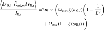$$\begin{array}{cc}\hfill \frac{\langle {\mathit{\delta }\mathit{r}}_{0,i},{\widehat{\mathcal{L}}}_{\mathrm{rot},m}{\mathit{\delta }\mathit{r}}_{0,i}\rangle }{I_{0,i}}=& 2m\times ({\mathrm{\Omega }}_{\mathrm{core}}\zeta ({\omega }_{0,i})(1-\frac{1}{L^2})\hfill \\ \hfill & +{\mathrm{\Omega }}_{\mathrm{env}}(1-\zeta ({\omega }_{0,i}))).\hfill \end{array}$$(16)

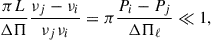
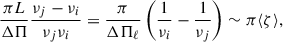
We use this description, excluding near-degeneracy effects (i.e. off-diagonal near-degeneracy terms), to fit the ℓ = 1 modes in Sect. 4 because the targets we chose have a large frequency separation, Δν > 20, where we expect little to no influence of near-degeneracy effects (Ahlborn et al. 2025). In the case of more evolved stars in the regime of low asymmetry splittings (typically for 11 < Δν < 13, depending on the core rotation rate according to Ahlborn et al. 2025), our framework provides an explicit second-order perturbative correction to the rotational splitting (based on Eq. (27), see Appendix A for more details).

This approach eliminates the need to solve the implicit equation used by Li et al. (2024) to reproduce the rotational asymmetries in ℓ = 1 mode splittings.

2.3. Near-degeneracy effects: Non-diagonal terms

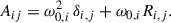
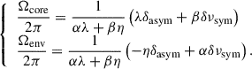
The symmetry in the splitting of the modes can be broken when the non-diagonal elements (i.e. i ≠ j) of the matrix, R, become non-negligible compared to the diagonal. This is expected to happen when two modes have a frequency separation comparable to the rotation rate of the star, i.e. when |ω_i − ω_j|∼Ω (Dziembowski & Goode 1992; Deheuvels et al. 2017; Ahlborn et al. 2025). This is illustrated in Fig. 1, which uses the asymptotic framework of this paper to highlight how near-degenerate interactions modify the usual pattern of rotationally split multiplets and generate asymmetries in the frequency pattern.

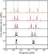Fig. 1. Illustration of the effect of near degeneracy on two coupled ℓ = 2 multiplets as the core rotation rate νc = Ωcore/2π increases for a fixed inclination angle of i = 42°. Each horizontally modelled PSD shows the combined visibility profile of the ten components (two sets of m = −2, −1, 0, +1, +2 modes) at a given νc. The greyscale background indicates how the multiplet structure evolves continuously with rotation.

The off-diagonal terms, which are those responsible for the near-degeneracy asymmetry effects, can be written as (Deheuvels et al. 2017)

$$\begin{array}{c}\hfill \frac{\langle {\mathit{\delta }\mathit{r}}_{0,i},{\widehat{\mathcal{L}}}_{\mathrm{rot},m}{\mathit{\delta }\mathit{r}}_{0,j}\rangle }{\sqrt{I_{0,i}{I}_{0,j}}}=2m({\gamma }_{c,ij}{\mathrm{\Omega }}_{\mathrm{core}}+{\gamma }_{e,ij}{\mathrm{\Omega }}_{\mathrm{env}}),\end{array}$$(17)

with

$$\begin{array}{c}\hfill {\gamma }_{c,ij}=\frac{1}{\sqrt{I_{0,i}{I}_{0,j}}}{\displaystyle {\int }_{\mathrm{g}}}{K}_{i,j}(r)\mathrm{d}r\end{array}$$(18)

and

$$\begin{array}{c}\hfill {\gamma }_{e,ij}=\frac{1}{\sqrt{I_{0,i}{I}_{0,j}}}{\displaystyle {\int }_{\mathrm{p}}}{K}_{i,j}(r)\mathrm{d}r.\end{array}$$(19)

Because the mixed-mode basis is orthogonal and the oscillation verify ξ_r ≪ ξ_h (resp. ξ_r ≫ ξ_h) in the g-mode cavity (resp. p-mode cavity) (e.g. Aerts et al. 2010; Bugnet et al. 2021; Mathis et al. 2021), Deheuvels et al. (2017) showed that

$$\begin{array}{c}\hfill {\gamma }_{c,ij}=\frac{1}{\sqrt{I_{0,i}{I}_{0,j}}}{\displaystyle {\int }_{\mathrm{g}}}\rho r^2(L^2-1){\xi }_{0,h,i}^{\ast }{\xi }_{0,h,j}\mathrm{d}r,\end{array}$$(20)

and

$$\begin{array}{c}\hfill {\gamma }_{e,ij}=\frac{L^2}{1-L^2}{\gamma }_{c,ij}.\end{array}$$(21)

Hence, in order to describe the off-diagonal terms of the eigenvalue problem, it is sufficient to evaluate γ_c, ij.

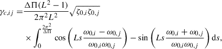
2.3.1. New asymptotic formula for the near degeneracy effects

To find an asymptotic formula for γ_c, ij that could be applied to fit observations, we used the asymptotic Jeffreys-Wentzel–Kramers–Brillouin (e.g. Jeffreys 1925; Wentzel 1926) form of the horizontal eigenfunctions in the g-mode cavity as given in, for example, Mathis et al. (2021):

$$\begin{array}{c}\hfill {\xi }_h=-\frac{A}{\sqrt{L}\omega }{\rho }^{-1/2}{r}^{-3/2}{\left(\frac{N^2}{{\omega }^2}\right)}^{1/4}sin(L{\displaystyle {\int }_0^r}\frac{N}{\omega }\frac{\mathrm{d}r\prime }{r\prime }-\frac{\pi }{4}),\end{array}$$(22)

where A is the amplitude of the mode and N is the Brunt–Väisälä frequency. This yields

$$\begin{array}{cc}\hfill {\gamma }_{c,ij}=& \frac{1}{\sqrt{I_{0,i}{I}_{0,j}}}{\displaystyle {\int }_{\mathrm{g}}}\frac{A_{0,i,g}{A}_{0,j,g}(L^2-1)}{L\sqrt{{\omega }_{0,i}^3{\omega }_{0,j}^3}}\frac{N}{r}\hfill \\ \hfill & \times sin(L{\displaystyle {\int }_0^r}\frac{N}{r\prime }\mathrm{d}r\prime \frac{1}{{\omega }_{0,i}}-\frac{\pi }{4})sin(L{\displaystyle {\int }_0^r}\frac{N}{r\prime }\mathrm{d}r\prime \frac{1}{{\omega }_{0,j}}-\frac{\pi }{4})\mathrm{d}r.\hfill \end{array}$$(23)

Asymptotically, the inertia of the mode in the g-mode cavity can be written as (e.g. Hekker & Christensen-Dalsgaard 2017)

$$\begin{array}{c}\hfill I_g=\frac{A_g^2{\pi }^{2}L}{{\omega }^3\mathrm{\Delta }\mathrm{\Pi }}\iff A_g=\sqrt{\frac{\mathrm{\Delta }\mathrm{\Pi }{\omega }^3{I}_g}{L{\pi }^2}},\end{array}$$

with $\mathrm{\Delta }\mathrm{\Pi }=\sqrt{\ell (\ell +1)}\mathrm{\Delta }{\mathrm{\Pi }}_{\ell }$ as the reduced period spacing of the g modes. This yields the following result:

$$\begin{array}{cc}\hfill {\gamma }_{c,ij}=& \frac{1}{\sqrt{I_{0,i}{I}_{0,j}}}{\displaystyle {\int }_{g\mathrm{cavity}}}\frac{\mathrm{\Delta }\mathrm{\Pi }(L^2-1)}{L^2{\pi }^2}\sqrt{I_{0,g,i}{I}_{0,g,j}}\frac{N}{2r}\hfill \\ \hfill & \times [cos(L{\displaystyle {\int }_0^r}\frac{N}{r\prime }\mathrm{d}r\prime \frac{{\omega }_{0,j}-{\omega }_{0,i}}{{\omega }_{0,i}{\omega }_{0,j}})\hfill \\ \hfill & -sin(L{\displaystyle {\int }_0^r}\frac{N}{r\prime }\mathrm{d}r\prime \frac{{\omega }_{0,j}+{\omega }_{0,i}}{{\omega }_{0,i}{\omega }_{0,j}})]\mathrm{d}r.\hfill \end{array}$$(24)

Here, we have used the trigonometric identity $sin(a)sin(b)=\frac{1}{2}(cos(a-b)-cos(a+b))$. Using the change of variable¹

$$\begin{array}{c}\hfill s={\displaystyle {\int }_0^r}\frac{N}{r\prime }\mathrm{d}r\prime \end{array}$$(25)

and using the seismic ζ function leads to the following expression:

$$\begin{array}{cc}\hfill {\gamma }_{c,ij}=& \frac{\mathrm{\Delta }\mathrm{\Pi }(L^2-1)}{2{\pi }^2{L}^2}\sqrt{{\zeta }_{0,i}{\zeta }_{0,j}}\hfill \\ \hfill & \times {\displaystyle {\int }_0^{\frac{2{\pi }^2}{\mathrm{\Delta }\mathrm{\Pi }}}}cos\left(Ls\frac{{\omega }_{0,i}-{\omega }_{0,j}}{{\omega }_{0,i}{\omega }_{0,j}}\right)-sin\left(Ls\frac{{\omega }_{0,i}+{\omega }_{0,j}}{{\omega }_{0,i}{\omega }_{0,j}}\right)\mathrm{d}s,\hfill \end{array}$$(26)

where we have used the fact that by definition of ΔΠ, s(r_core) = 2π²/ΔΠ. This was integrated to

$$\begin{array}{cc}\hfill {\gamma }_{c,ij}=& \frac{\mathrm{\Delta }\mathrm{\Pi }(L^2-1)}{\pi L^3}\sqrt{{\zeta }_{0,i}{\zeta }_{0,j}}\times [\frac{{\nu }_{0,i}{\nu }_{0,j}}{{\nu }_{0,j}-{\nu }_{0,i}}sin\left(\frac{\pi L}{\mathrm{\Delta }\mathrm{\Pi }}\frac{{\nu }_{0,j}-{\nu }_{0,i}}{{\nu }_{0,j}{\nu }_{0,i}}\right)\hfill \\ \hfill & +\frac{{\nu }_{0,i}{\nu }_{0,j}}{{\nu }_{0,j}+{\nu }_{0,i}}(cos\left(\frac{\pi L}{\mathrm{\Delta }\mathrm{\Pi }}\frac{{\nu }_{0,j}+{\nu }_{0,i}}{{\nu }_{0,j}{\nu }_{0,i}}\right)-1)],\hfill \end{array}$$(27)

where we have expressed the quantities as a function of the frequency ν = ω/2π for ease of implementation.

An important point to highlight is that the quantity γ_c, ij, which we derived in this work as part of a new asymptotic formulation including off-diagonal rotational near-degeneracy terms, is expressed using the exact same asymptotic parameters traditionally used in first-order symmetric splitting approaches (i.e. in the characterisation of mixed ℓ = 2 modes, ΔΠ₂ replaces ΔΠ₁ and ζ₂ replaces ζ from the frameworks of Mosser et al. 2012a; Goupil et al. 2013; Deheuvels et al. 2014). This shows that we can achieve a better degree of precision on core and envelope rotation measurements by including additional constraints from ℓ = 2 modes without the need to change the usual formalism and analysis tools.

Our asymptotic formulation in Eq. (27) can be compared with the derivation of Ong et al. (2022) in the π − γ decoupled mode basis. When the argument of the sin in γ_c, ij is small, i.e.

$$\begin{array}{c}\hfill \frac{\pi L}{\mathrm{\Delta }\mathrm{\Pi }}\frac{{\nu }_j-{\nu }_i}{{\nu }_j{\nu }_i}=\pi \frac{P_i-P_j}{\mathrm{\Delta }{\mathrm{\Pi }}_{\ell }}\ll 1,\end{array}$$(28)

where P_i (resp. P_j) is the period of the mode i (resp j), Eq. (27) becomes equivalent to ${\gamma }_c\approx \frac{L^2-1}{L^2}\sqrt{{\zeta }_i{\zeta }_j}$ when using a first-order Taylor expansion. This gives ${\gamma }_e\approx -\sqrt{{\zeta }_i{\zeta }_j}$. This last approximation yields a result that connects to Eq. (35) of Ong et al. (2022). This situation is most frequent around p-dominated mixed modes. Indeed for two consecutive mixed modes,

$$\begin{array}{c}\hfill \frac{\pi L}{\mathrm{\Delta }\mathrm{\Pi }}\frac{{\nu }_j-{\nu }_i}{{\nu }_j{\nu }_i}=\frac{\pi }{\mathrm{\Delta }{\mathrm{\Pi }}_{\ell }}(\frac{1}{{\nu }_i}-\frac{1}{{\nu }_j})\sim \pi ⟨\zeta ⟩,\end{array}$$(29)

where

$$\begin{array}{c}\hfill ⟨\zeta ⟩=(\frac{1}{{\nu }_i}-\frac{1}{{\nu }_j}){\left({\displaystyle {\int }_{\frac{1}{{\nu }_j}}^{\frac{1}{{\nu }_i}}}\frac{\mathrm{d}P}{\zeta (P)}\right)}^{-1},\end{array}$$(30)

with P = 1/ν following Mosser et al. (2015) (see their Eq. (12)). Hence, for a small ⟨ζ⟩ (or equivalently a very p-dominated couple of modes), the quantity π⟨ζ⟩ will be small. On the contrary, in the far resonance limit, when

$$\begin{array}{c}\hfill \frac{\pi L}{\mathrm{\Delta }\mathrm{\Pi }}\frac{{\nu }_j-{\nu }_i}{{\nu }_j{\nu }_i}\gg 1,\end{array}$$(31)

the non-diagonal terms become negligible compared to the diagonal ones, and we recover symmetrical splittings.

2.3.2. Validation of the new asymptotic formula for near degeneracy effects

To further determine the validity of our new asymptotic formulation of near-degeneracy effects, we sought to reproduce the results of Deheuvels et al. (2017). To do so, we used exactly the same input parameters adopted in their study, only allowing the core and envelope rotation rates to be free (Eq. 17).

To date, KIC 7341231 is the only star in which the near-degeneracy effects of ℓ = 2 modes have been characterised in detail in one radial order. In their analysis, Deheuvels et al. (2017) adopted a different approach from ours: They computed a 1D stellar model using Cesam2k (Morel 1997) while assuming a two-zone rotation profile. They then explicitly computed γ_c from the rotational kernels and solved the full eigenvalue problem. In contrast, our work relies on a fully parametrised asymptotic formulation of γ_c, which allows us to directly compare our results with those obtained from their numerical approach. Specifically, we fitted the core and envelope rotation rates of the two-zone model based on the ℓ = 2, m = ±2 rotational splittings obtained from their peakbagging analysis of two ℓ = 2 multiplets a and b (see their Table 1), together with the m = 0 mode frequencies (ν_0, a and ν_0, b) and the corresponding trapping fractions ζ_a and ζ_b reported in their Table 3. To compute the m = ±2 components of each mixed a and b, we evaluated the eigenvalues of the following matrix, as done by Deheuvels et al. (2017) in their Appendix A:

$$\begin{array}{c}\hfill \left[\begin{array}{cc}{\nu }_{0,a}^2+2{\nu }_{0,a}\frac{⟨{\mathit{\delta }\mathit{r}}_{0,a},{\widehat{\mathrm{L}}}_{\mathrm{rot},m}{\mathit{\delta }\mathit{r}}_{0,a}⟩}{2\pi {\mathrm{I}}_{0,\mathrm{a}}}& 2{\nu }_{0,a}\frac{⟨{\mathit{\delta }\mathit{r}}_{0,a},{\widehat{\mathrm{L}}}_{\mathrm{rot},m}{\mathit{\delta }\mathit{r}}_{0,b}⟩}{2\pi \sqrt{{\mathrm{I}}_{0,\mathrm{a}}{\mathrm{I}}_{0,\mathrm{b}}}}\\ 2{\nu }_{0,b}\frac{⟨{\mathit{\delta }\mathit{r}}_{0,b},{\widehat{\mathrm{L}}}_{\mathrm{rot},m}{\mathit{\delta }\mathit{r}}_{0,a}⟩}{2\pi \sqrt{{\mathrm{I}}_{0,\mathrm{a}}{\mathrm{I}}_{0,\mathrm{b}}}}& {\nu }_{0,b}^2+2{\nu }_{0,b}\frac{⟨{\mathit{\delta }\mathit{r}}_{0,b},{\widehat{\mathrm{L}}}_{\mathrm{rot},m}{\mathit{\delta }\mathit{r}}_{0,b}⟩}{2\pi {\mathrm{I}}_{0,\mathrm{b}}}\end{array}\right].\end{array}$$(32)

This formulation is an approximation of (9) introduced by Deheuvels et al. (2017). Since they use this approximated form in their article, we choose to do the same when vetting our results in order to stay as close to the article as possible. This is the only part of the present work in which we compute the splittings due to near-degeneracy effects with this approximation; in the rest of our work, we solve the full quadratic eigenvalue problem (9).

In our formulation, the off-diagonal elements of this matrix were computed using Eq. (27), while the diagonal terms were derived from Eq. (16) (Goupil et al. 2013; Deheuvels et al. 2014).

The values and uncertainties on the inferred core and envelope rotation rates were estimated using a Monte Carlo approach. The resulting values are shown in Fig. B.1. Using identical mixed-mode parameters but replacing their numerical model with our asymptotic formulation, we achieved an excellent agreement with the published results. We obtained Ω_core/2π = 772 ± 9 nHz and Ω_env/2π = 45 ± 6 nHz, while Deheuvels et al. (2017) reported Ω_core/2π = 771 ± 13 nHz and Ω_env/2π = 45 ± 12 nHz. The close agreement between the two methods confirms that the asymptotic formulation provides a robust and accurate description of the observed rotational splittings and can be used to analyse asteroseismic observations of ℓ = 2 modes without the need of numerical models. Our fitted measurement also hints at our approach being able to obtain better precision, which we confirm in Section 4.

3. Data analysis framework

Our next aim was to apply the asymptotic formalism described by Eqs. (16), (17) and (27) in order to perform global fits of the PSD, thereby constraining the mixed-mode parameters and the core as well as envelope rotation rates while using all available data. In particular, we deliberately avoided performing peakbagging prior to the model fitting, as whether a given peak represents a genuine oscillation mode or merely stochastic noise can often be ambiguous. The main advantage of fitting the PSD directly with a physically informed model based on asymptotic relations is that the distinction between signal and noise naturally emerges from the fit itself without requiring any subjective preselection of peaks.

To accomplish this, we employed a Markov chain Monte Carlo approach within a Bayesian framework to fit the oscillation modes in the PSD. The p- and mixed-mode patterns were created using the sloscillations code developed in Kuszlewicz et al. (2019, 2023), which was extended to incorporate the near-degeneracy effects based on Section 2. How the synthetic PSD was generated is described in Sect. 3.1 below.

3.1. Synthetic power spectral density

3.1.1. Description of the set-up of the asymptotic model

The asymptotic model used in the fitting procedure predicts the full oscillation spectrum from a set of physically motivated parameters. For each angular degree ℓ ∈ {0, 1, 2}, the model generates the underlying p- and g-mode frequencies from the asymptotic relations described below, which are then coupled through the mixed-mode formalism and corrected for rotational splitting at first order (for ℓ = 1) or through the full quadratic eigenvalue problem (for ℓ = 2).

The free parameters of the model therefore include the global p-mode pattern parameters (Δν, ε, δν_0, ℓ, α, β_0, ℓ); the g-mode period-spacing and phase parameters (ΔΠ_ℓ, ε_g, ℓ); the p–g coupling strengths (q_ℓ); and the core and envelope rotation rates (Ω_core, Ω_env) as well as the stellar inclination angle (θ_inc).

Each predicted mode is assigned a Lorentzian profile with an analytically prescribed linewidth and height, and these components are summed together with a synthetic granulation and white-noise background to produce a fully specified model of the PSD.

3.1.2. Pure pressure and gravity modes

The pure p modes were computed using the following equation (e.g. Tassoul 1980; Elsworth et al. 1990; Mosser et al. 2011; Lund et al. 2017; Breton et al. 2022):

$$\begin{array}{cc}& {\nu }_{\mathrm{p};\mathrm{n},\ell }=\hfill \\ \hfill & (n+\frac{\ell }{2}+\epsilon +{\beta }_{0,\ell }(n-n_{\max })+\frac{\alpha }{2}{(n-n_{\max })}^2)\mathrm{\Delta }\nu -\delta {\nu }_{0,\ell },\hfill \end{array}$$(33)

where n_max is the order of the mode of maximum power, ε is the global p-mode phase shift, and δν_0, ℓ is the frequency shift of the modes from their first order asymptotic position (Tassoul 1980). To capture the frequency dependence of Δν and δν_0, ℓ, α and β_0, ℓ are introduced ad hoc (Elsworth et al. 1990; Lund et al. 2017; Breton et al. 2022). The pure g modes were computed using (e.g. Tassoul 1980)

$$\begin{array}{c}\hfill {\nu }_{\mathrm{g};\mathrm{n},\ell }=\frac{1}{\mathrm{\Delta }{\mathrm{\Pi }}_{\ell }(n+\frac{1}{2}+{\epsilon }_{\mathrm{g}})},\end{array}$$(34)

where ε_g is the phase shift of the g modes.

3.1.3. Mixed modes with rotation

Unperturbed mixed-mode frequencies were computed using the following equation (Shibahashi 1979):

$$\begin{array}{c}\hfill \mathrm{cotan}({\mathrm{\Theta }}_{\mathrm{g}})tan({\mathrm{\Theta }}_{\mathrm{p}})=q_{\ell }\end{array}$$(35)

with (Ong & Gehan 2023)

$$\begin{array}{cc}& {\mathrm{\Theta }}_{\mathrm{p}}=\frac{\pi }{\mathrm{\Delta }\nu }(\nu -{\nu }_{\mathrm{p}}),\hfill \\ \hfill & {\mathrm{\Theta }}_{\mathrm{g}}=\frac{\pi }{2}-\frac{\pi }{\mathrm{\Delta }{\mathrm{\Pi }}_{\ell }}(\frac{1}{{\nu }_{\mathrm{g}}}-\frac{1}{\nu }),\hfill \end{array}$$(36)

and where q_ℓ is the coupling factor between the p- and g- modes for the corresponding order ℓ (we expect q₂ < q₁ due to the shallower p-mode cavity for ℓ = 2 modes).

We introduced the effects of rotation on the unperturbed frequencies at the first perturbative order for the ℓ = 1 components and solved the full rotating quadratic eigenvalue problem Eq. (9) with asymptotic matrix elements for ℓ = 2 (based on our asymptotic formulation Eq. (27)) modes using the slepc4py (Hernandez et al. 2005; Dalcin et al. 2011) Python library.

When computing the off diagonal elements of the rotation matrix, we used the asymptotic formula for ζ defined in Eq. (15) such that (Goupil et al. 2013; Deheuvels et al. 2015; Hekker & Christensen-Dalsgaard 2017)

$$\begin{array}{c}\hfill \zeta (\nu )={[1+\frac{{\nu }^2\mathrm{\Delta }{\mathrm{\Pi }}_{\ell }}{\mathrm{\Delta }\nu }\frac{1}{q{cos}^2({\mathrm{\Theta }}_p)+\frac{1}{q}{sin}^2({\mathrm{\Theta }}_p)}]}^{-1}\end{array}$$(37)

while using the above definition of Θ_p.

3.1.4. Modelling the linewidths, amplitudes, and heights of the modes

This paragraph describes the equations and methodologies used to compute the linewidths, amplitudes, and heights of the modes in the sloscillations code by Kuszlewicz et al. (2019) for the sake of completeness and clarity. These parameters were fully derived from scaling relations and analytical expressions and are thus not fitted parameters in the model. We adopted effective-temperature-dependent scaling relations for the p-mode linewidths, parametrised as a function of temperature, following the empirical prescriptions of Corsaro et al. (2012), Lund et al. (2017). The radial-mode amplitudes follow a Gaussian envelope centred on ν_max, with width tied to the envelope full width at half maximum and a peak amplitude that scales with global parameters (ν_max, Δν). The per-degree amplitudes were set by standard photometric visibilities as in Kuszlewicz et al. (2019) and, for non-radial multiplets, by geometric inclination (θ_inc) factors (Gizon & Solanki 2003). For mixed ℓ = 1 and ℓ = 2 modes, we modulated the nominal p-mode amplitudes by ${(1-\zeta )}^{\frac{1}{2}}$ (Mosser et al. 2018; Basu & Chaplin 2017). The mode heights in the power spectrum were computed from the time-domain amplitudes and the linewidths using the finite-observation-length correction of Fletcher et al. (2006). For mixed modes, we used the mixed-mode generalisation that explicitly includes the inertia ratio ζ (Basu & Chaplin 2017), ensuring that g-dominated mixed modes appear with an appropriately reduced height at a fixed amplitude. Each mode contributes a Lorentzian profile to the PSD, centred at the asymptotic frequency and with the height and width described above.

The background of the synthetic PSD was modelled with the usual super-Lorentzian granulation components and white noise (e.g Kallinger et al. 2014). It was generated in the time domain via a Gaussian-process representation of convection and granulation following Kuszlewicz et al. (2019), where a kernel encapsulates the covariance of stochastic surface motions (e.g. Foreman-Mackey et al. 2017; Pereira et al. 2019; O’Sullivan & Aigrain 2024). This data was Fourier transformed, and the resulting PSD provided the granulation floor plus white noise that forms the background in the PSD. On top of this background, the oscillation spectrum was added, producing a self-consistent synthetic PSD where both the convective noise and p-mode power originate from the same underlying time-domain process. During the fitting procedure, the synthetic background was then normalised using the same procedure applied to the observed data (see Sect. 4.1). Since the same background normalisation was applied consistently to both the observed and synthetic spectra, the fit remained statistically self-consistent and did not introduce any bias in the inferred mode frequencies.

3.2. Description of the Bayesian fitting procedure

3.2.1. Priors on p modes and ℓ = 1 mixed modes

Appendix C describes the method used to define prior ranges for the rotational, p-mode, and ℓ = 1 mixed-mode parameters. These ranges are guided by both theoretical expectations and previous observational studies.

3.2.2. Priors on the ℓ = 2 period spacing ΔΠ₂ and phase ε_g, 2

Using the fact that the period spacing ΔΠ = LΔΠ_ℓ is constant (Tassoul 1980), we obtained

$$\begin{array}{c}\hfill \mathrm{\Delta }{\mathrm{\Pi }}_2=\frac{\mathrm{\Delta }{\mathrm{\Pi }}_1}{\sqrt{3}}·\end{array}$$(38)

Hence, once we had measured ΔΠ₁, we chose to assign a flat prior within ±5% of the value of ΔΠ₂ from Eq. (38).

As for ε_g, 2, we have, to our knowledge, no theoretical grounds to constrain it. Hence, we chose to use an uninformative flat prior between zero and one, as done for ε_g, 1 (see Appendix C).

3.2.3. Priors on the ℓ = 2 modes coupling parameter q₂

We examined what constraints could be put on q₂, the coupling factor of ℓ = 2 modes, depending on the inclination angle of the star compared to the line of sight (θ_inc), which we estimated by the preliminary fit of the ℓ = 1 modes (Appendix C). When the ℓ = 2, m = 0 modes are visible, we used the technique described in Sect. 3.2.4. When the angle of inclination makes the ℓ = 2 and m = 0 modes not visible, we used the result of Sect. 3.2.5.

3.2.4. Priors on the ℓ = 2 modes coupling parameter q₂ using the m = 0 modes

Using Eq. (15) of Ong & Gehan (2023), we obtained that for two consecutive mixed modes (with the same ℓ order) of frequency ν_a and ν_b,

$$\begin{array}{cc}& arctan\left(\frac{tan\left({\mathrm{\Theta }}_{\mathrm{p},a}\right)}{q_{\ell }}\right)-arctan\left(\frac{tan\left({\mathrm{\Theta }}_{\mathrm{p},b}\right)}{q_{\ell }}\right)\hfill \\ \hfill & =\frac{\pi }{\mathrm{\Delta }{\mathrm{\Pi }}_{\ell }}(\frac{1}{{\nu }_a}-\frac{1}{{\nu }_b}+\mathrm{\Delta }{\mathrm{\Pi }}_{\ell }).\hfill \end{array}$$(39)

Using trigonometric relations, we show that this formula is equivalent to

$$\begin{array}{cc}& \frac{tan\left({\mathrm{\Theta }}_{\mathrm{p},a}\right)-tan\left({\mathrm{\Theta }}_{\mathrm{p},b}\right)}{q_{\ell }}\frac{1}{1+\frac{1}{q_{\ell }^2}tan\left({\mathrm{\Theta }}_{\mathrm{p},a}\right)tan\left({\mathrm{\Theta }}_{\mathrm{p},b}\right)}\hfill \\ \hfill & =-tan\left(\frac{\pi }{\mathrm{\Delta }{\mathrm{\Pi }}_{\ell }}(\frac{1}{{\nu }_b}-\frac{1}{{\nu }_a})\right),\hfill \end{array}$$(40)

which is conveniently a second-order polynomial in $\frac{1}{q_{\ell }}$.

Hence, by defining

$$\begin{array}{cc}& K=tan\left(\frac{\pi }{\mathrm{\Delta }{\mathrm{\Pi }}_{\ell }}(\frac{1}{{\nu }_b}-\frac{1}{{\nu }_a})\right)\hfill \\ \hfill & A=Ktan\left({\mathrm{\Theta }}_{\mathrm{p},a}\right)tan\left({\mathrm{\Theta }}_{\mathrm{p},b}\right)\hfill \\ \hfill & B=tan\left({\mathrm{\Theta }}_{\mathrm{p},b}\right)-tan\left({\mathrm{\Theta }}_{\mathrm{p},a}\right)\hfill \\ \hfill & \mathrm{\Delta }=B^2-4AK,\hfill \end{array}$$(41)

we obtained that q_ℓ is given by

$$\begin{array}{c}\hfill q_{\ell }=\frac{2A}{B+\sqrt{\mathrm{\Delta }}}·\end{array}$$(42)

In order to obtain q₂, we thus needed ΔΠ₂, Δν, ν_a, ν_b, and the position of the ℓ = 2 p mode that is obtained from the radial mode frequency and δν_0, 2.

3.2.5. Priors on the ℓ = 2 modes coupling parameter q₂ using the ℓ = 1 mode coupling parameter q₁

When the inclination angle of the rotation axis is such that the m = 0 components of the multiplet splittings are not visible, we cannot use the above method to yield an estimate of q₂. Indeed the previous method relies on the frequencies of the pure mixed modes not affected by dynamical processes, which is not the case for the components of a multiplet with |m|> 0. Hence, we derived an upper bound of q₂ as a function of q₁. In order to do so, we used the approximation that in the evanescent zone, N ≪ ω ≪ S_ℓ, where N is the Brunt-Väisälä frequency and S_ℓ the Lamb frequency. In the approximation of a thick evanescent zone, the transmission coefficient can be approximated as (Unno et al. 1989; Takata 2016a)

$$\begin{array}{c}\hfill t_{\ell ,\mathrm{thick}}\approx {\left(\frac{r_0}{r_{\ell }}\right)}^L,\end{array}$$(43)

where r₀ is the turning point between the g-mode cavity and the evanescent zone, which is independent of ℓ, and r_ℓ is the turning point at the limit between the evanescent zone and the p-mode cavity.

While this thick evanescent zone approximation may not be applicable to ℓ = 1 modes, we know from Takata (2016b) that t_ℓ, thick > t_ℓ, thin, where t_ℓ, thin is the transmission coefficient computed with the asymptotic equation that is appropriate when the evanescent zone is thin (Takata 2016b; van Lier et al. 2025). Hence, this approximation is appropriate in the search of an upper boundary on q₂. At fixed frequency, the monotonic increase of S_ℓ with ℓ implies r₂ > r₁ and therefore

$$\begin{array}{c}\hfill t_2\approx {\left(\frac{r_0}{r_2}\right)}^{\sqrt{6}}<{\left(\frac{r_0}{r_1}\right)}^{\sqrt{6}}\approx t_1^{\sqrt{3}}.\end{array}$$(44)

Using the fact that (Takata 2016a)

$$\begin{array}{c}\hfill q_{\ell }=\frac{1-\sqrt{1-t_{\ell }^2}}{1+\sqrt{1-t_{\ell }^2}},\end{array}$$(45)

We finally obtain

$$\begin{array}{c}\hfill q_2<\frac{1-\sqrt{1-{\left(\frac{4q_1}{{(q_1+1)}^2}\right)}^{\sqrt{3}}}}{1+\sqrt{1-{\left(\frac{4q_1}{{(q_1+1)}^2}\right)}^{\sqrt{3}}}}·\end{array}$$(46)

3.2.6. Likelihood adopted in the Markov chain Monte Carlo approach

In our Markov chain Monte Carlo approach, we adopted the likelihood appropriate for a power spectrum whose noise follows a χ² distribution with two degrees of freedom (Woodard 1984; Toutain & Appourchaux 1994; Breton et al. 2022). The corresponding log-likelihood is

$$\begin{array}{c}\hfill ln\mathcal{L}=-{\displaystyle \sum _i}[\frac{P_i}{M_i}+ln{M}_i],\end{array}$$

where P_i denotes the observed power and M_i is the model power at a frequency bin i. The Bayesian inference procedure then adjusts the asymptotic parameters so as to maximise this likelihood, thereby ensuring that the resulting synthetic PSD matches the observed one as closely as possible. The different components of the model are presented in the paragraphs above.

3.2.7. Adopted fitting strategy

In order to fit the asymptotic pattern to asteroseismic data, we used a three-step approach. (i) In order to find priors on pressure mode parameters, we ran the global asteroseismic code PyA2Z (Liagre et al., in prep., based on the A2Z code Mathur et al. 2010), which gives guesses of the large frequency separation, Δν; the frequency of maximum power, ν_max; and the p-mode phase shift, ε (as well as the period spacing, ΔΠ₁, of ℓ = 1 g modes). (ii) We fitted the radial mode pattern and the first order split ℓ = 1 mixed-mode pattern following Sect. C.1 (i.e. we fitted Δν, ε, δν_0, 1, α, ΔΠ₁, q₁, ε_g, 1, Ω_core, Ω_env, β_0, 1, and θ_inc, which is the inclination angle of the rotation axis compared to the line of sight for KIC 8179973) to get the parameters needed to obtain priors on ℓ = 2 modes from Eqs. (38), (42), and (46). (iii) Once we had the priors on all parameters (listed in Table C.1), we performed the global asymptotic fit of the PSD (ℓ = 0, 1, 2 modes with rotation) following Appendices C.2 and C.3. We chose not to include ℓ ≥ 3 modes in our model, as their amplitudes are very small.

While the mixed ℓ = 1 mode parameters and pressure mode parameters were already fitted in the first two steps of the procedure, we chose not to freeze them during the global fit to avoid biases in the inferred rotational and l = 2 parameters. This resulted in a global fit, the corner plot of which can be found in Appendix C.4.

4. The first asymptotic fits of near-degeneracy effects in quadrupolar mixed modes

4.1. Selection of candidates and data pre-processing

The first target we used to validate this new asymptotic formulation of asymmetric rotational splitting is the one studied with a numerical modelling approach by Deheuvels et al. (2017): KIC 7341231. In order to find additional targets with mixed ℓ = 2 modes on which to apply our formulation of asymmetric rotational splittings, we chose to focus on stars in the early red giant or late sub-giant evolutionary stage, as they are expected to exhibit higher coupling factors for both ℓ = 1 and ℓ = 2 modes than more evolved stars. A convenient sample for exploring this evolutionary phase is in Liagre et al. (2025), who re-analysed aliased asteroseismic data from ≈2000 long cadence Kepler light curves and found a new sample of ≈350 young red giants with ν_max above or close to the Nyquist frequency of the Kepler long cadence data. While the sample presented in Liagre et al. (2025) contains more than 300 stars with pulsations above the Nyquist frequency and hence in the early red giant evolutionary stage, we wanted to analyse stars with a short-cadence timeseries to avoid misinterpreting aliased peaks as modes and with sufficient resolution and a signal-to-noise ratio to work well with our fitting procedure. This significantly reduced the available number of targets, and among those, we found that KIC 8179973 was the most promising, as a visual inspection of the echelle diagram of the star showed clear ℓ = 2 avoided crossings. We therefore selected KIC 8179973 as another good candidate for a global fit of ℓ = 1, 2 mixed modes including near-degeneracy effects, as it exhibits mixed ℓ = 2 modes with an exceptional signal-to-noise ratio.

The seismic analyses were done using short-cadence Kepler light curves filtered at 20 days and were obtained from the Mikulski Archive for Space Telescopes (MAST) archive. They were corrected with the Kepler Asteroseismic Data Analysis and Calibration Software (KADACS; García et al. 2011) to remove outliers, correct any jumps and drifts, and stitch together the quarters. All the observational gaps were interpolated using in-painting techniques based on a multi-scale discrete cosine transform (García et al. 2014; Pires et al. 2015). We isolated the oscillatory signal in the PSD from the granulation background, which dominates the PSD at frequencies around ν_max. We implemented the background normalisation procedure using the empirical scaling relation established in Mosser et al. (2012b):

$$\begin{array}{c}\hfill \mathrm{PSD}(\mathrm{SNR})=\frac{P}{\left({\nu }_{\max }^{-2.41}\right){\left(\frac{\nu }{{\nu }_{\max }}\right)}^{-2.1}6.37\times {10}^6},\end{array}$$(47)

where P represents either the observed or the synthetic power spectrum density. This normalisation effectively flattens the granulation background while preserving the relative amplitudes of the oscillation modes. Subsequently, we isolated the region of interest around ν_max (the extracted frequency window spans ν_max − 3Δν ≤ ν_max ≤ ν_max + 4Δν).

4.2. Results of the Bayesian asymptotic fitting

Figures 2 and 3 show the results of the fitting procedure described in Section 3 obtained for the two stars. The results are also reported in Table 1 along with the 1σ uncertainties extracted from the Bayesian analysis (the corner plots of the final fits can be found in Appendix C.4). When the posterior was asymmetrical, we chose to report the highest value of uncertainty as the error bar.

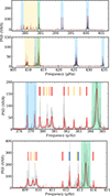Fig. 2. Asymptotic fit of KIC 7341231. In both panels, the Kepler data are in grey, and our asymptotic fit is in red. The radial, ℓ = 1, and ℓ = 2 modes are highlighted by the shading in green, blue, and yellow, respectively. Panel a: Two orders showing mixed ℓ = 2 modes with asymmetric splittings. Panel b: Zoom near 411 μHz on split ℓ = 2 modes. The m = 0, ±1, and ±2 components are marked in yellow, orange, and red. Panel c: Zoom near 381 μHz on split ℓ = 2 modes. The model is shown with thick red lins, data are in grey. The m = 0, ±1, and ±2 components of the ℓ = 2 mode are marked in yellow, orange, and red, and the m = ±1 components of the ℓ = 1 mode are marked in dark blue.

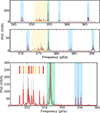Fig. 3. Asymptotic fit of KIC 8179973. In both panels, the Kepler data are in grey, and our asymptotic fit is in red. The radial, ℓ = 1, and ℓ = 2 modes are highlighted by the shading in green, blue, and yellow, respectively. Panel a: Two orders showing mixed ℓ = 2 modes with asymmetric splittings. Panel b: Zoom near 352 μHz on split near-degenerate ℓ = 2 modes. The quadrupolar mixed m = 0, ±1, and ±2 components are marked in yellow, orange, and red, respectively. The full fit can be found in Fig. C.7.

4.2.1. KIC 7341231

In Figure 2, we show our global fit of the mixed modes of KIC 7341231 and highlight in panels b and c the identification of ℓ = 2 modes on two consecutive radial orders. We vetted the asymptotic formula and fitting framework by comparing the results with the work of Deheuvels et al. (2017), which made use of complete evolutionary models of the star to analyse the radial order represented in panel b. We show that our fit is consistent with all visible ℓ = 2 modes in the PSD, as first identified in Fig. 1 of Deheuvels et al. (2017) in the neighbourhood of 380 μHz.

Apart from the specific radial order analysed by Deheuvels et al. (2017) in the vicinity of 380 μHz, the asymptotic fit allows for systematic identification of ℓ = 2 modes across the four surrounding radial orders (see Fig. C.4), which is a first for this star. In addition, we were able to properly identify multiplet components even when modes overlap between different angular degrees (ℓ). For instance, in Fig. 2 panels a and c, around 413 μHz, three modes of degree ℓ = 0, 1, 2 are superimposed, and each peak has been successfully identified individually through reconstruction of the asymptotic mode pattern.

In Table 2, we show that our estimate of core and envelope rotation rates are in agreement with model-based measurements from Deheuvels et al. (2017) and consistent across radial orders. We obtained about three times smaller uncertainties for the core rotation rate and two times smaller for the envelope rotation rate. This is due to the fact that our fit is global (as also performed for magnetic effects in Hatt et al. 2024). Indeed, uncertainties in mixed-mode parameters are usually estimated through non-parametric methods that do not exploit the full spectral information and instead consider errors on individual frequencies rather than the coherence of the global mixed-mode pattern (e.g. Gehan et al. 2018; Kuszlewicz et al. 2023). The global Bayesian fit also delivers better precision on asymptotic parameters in Table 1. For this reason, we advocate for broad use of these global fitting methods.

In order to assess the gain from adding constraints from ℓ = 2 modes to the fitting procedure, we estimated the Bayesian information criterion (BIC; Schwarz 1978) by comparing the fit performed with ℓ = 2 mixed modes and ℓ = 2 p modes only. To that end, we fitted the data again with split mixed dipole modes and pressure ℓ = 2 modes as usually done in the community and compared that restricted model against the full fit of the present work. The inclusion of mixed ℓ = 2 modes in the model leads to a BIC that is 3726 points lower than when using only mixed ℓ = 1 modes and pressure ℓ = 2 modes on the target KIC 7341231. Because the differences in the BIC approximate

$$\begin{array}{c}\hfill \mathrm{\Delta }\mathrm{BIC}\approx -2ln(\mathrm{BF}),\end{array}$$(48)

where BF is the bayes factor, such a large ΔBIC corresponds to overwhelmingly strong statistical evidence in favour of the extended model. We do not report the absolute BIC values themselves, as they are not tied to any absolute scale and carry no stand-alone interpretation. Only their differences have statistical meaning for model comparison. This substantial improvement in BIC therefore indicates very strong support for including the mixed ℓ = 2 modes, suggesting that the extended model provides a significantly better representation of the observed oscillation data. As a result, the physical inferences drawn from this model (such as internal rotation rates) can be considered significantly more robust and better constrained than those inferred from mixed ℓ = 1 modes only.

4.2.2. KIC 8179973

We performed the first fit of the radial and ℓ = 1, 2 mixed-mode pattern for KIC 8179973. This star presents a particularly asymmetric pattern in the ℓ = 2 regions, as the multiplets are very close to each other (see panels a and b of Fig. 3). The asymptotic prescription (Eq. 27) yields a very good interpretation of the PSD, with all visible modes being accurately represented (see also Fig. C.7). The values of ΔΠ₁, ε_g, 1, and q₁ are also in the range of the expected values from scaling relations and measurements of Mosser et al. (2017a), Kuszlewicz et al. (2023). The small number of visible mixed ℓ = 2 modes is expected based on the small mixed-mode density parameter (Gehan et al. 2018) 𝒩₂ = Δν/(ΔΠ₂ν_max²)≈3.4 and the fact that the coupling factor (q₂) is very small. Furthermore, for this star, we used a much less informative prior for q₂, as in the fit of KIC 7341231, which shows the robustness of our fitting method. In addition, ΔΠ₂ and ΔΠ₁ are compatible within 2σ following Eq. (38). From the global fit, we obtained Ω_core = 671 ± 8 μHz and Ω_env = 49 ± 8 μHz, which are within the expected range for a young red giant star (Gehan et al. 2018).

As for KIC 7341231, the uncertainties we obtained on KIC 8179973 are significantly smaller than those typically reported in similar studies (see e.g. Gehan et al. 2018; Deheuvels et al. 2014). This improvement highlights the strength of our global fitting procedure, which (i) minimises the uncertainties by simultaneously exploiting information from multiple modes and (ii) naturally mitigates the ambiguity between noise and genuine power excesses thanks to the intrinsic pattern constraints of the analysis. Compared to a fit that includes only the pure ℓ = 2 p modes, the BIC derived from the full asymptotic framework is lower by 3185 points. This provides strong statistical evidence that the prescription including mixed quadrupole modes and incorporating near-degeneracy effects offers a superior inference of the underlying physical parameters. This measurement of near-degeneracy effects in a second early red giant paves the way for a fully automated fitting pipeline based on asymptotic mixed-mode parameters across ℓ.

5. Conclusions

This work is the first to infer the complete set of asymptotic parameters of ℓ = 2 modes and the first to provide a fit of ℓ = 2 mode near-degeneracy splittings while not relying on a numerical model of the structure of a star. In particular, it has led to the first inferences of q₂, ΔΠ₂, and ε_g, 2, and with custom ways to constrain the coupling factor q₂, our work paves the way for an automation of the fit and identification of ℓ = 2 mixed modes.

Our results for ΔΠ₁ and ΔΠ₂ in KIC 8179973 are consistent within 2σ. However, in KIC 7341231, the values agree within a few tenths of a second with non-overlapping errors, suggesting either a small deviation from the asymptotic theory or the influence of surface effects that were not fully accounted for in this work. Indeed, because the fit of asymptotic mixed modes is very reliant on the position of the pure p-mode, a difference in the surface effects affecting the ℓ = 1 and ℓ = 2 notional p modes would suffice to explain a small difference in ΔΠ. In addition, our asymptotic formulation, including the ℓ = 2 modes, enabled us to put stronger constraints on the rotation rates of our targets. Indeed, in KIC 7341231 we measured an envelope (resp. core) rotation rate of 57 ± 11 nHz (resp. 777 ± 10 nHz) with only ℓ = 1 modes, while with the addition of ℓ = 2 modes combined with a global fitting framework, we obtained an envelope (resp. core) rotation of 53 ± 6 nHz (resp. 781 ± 4 nHz). Those values are compatible with each other, and we also observed that the inclusion of the mixed ℓ = 2 modes makes the uncertainty drop by a factor approximately equal to two (2.5 for the core rotation and 1.8 for envelope rotation). This is mostly due to the inclusion of more modes in the fitting procedure. There might also be a different contribution from the sensitivity kernels of the ℓ = 2 modes. Specifically, their shallower turning points offer distinct constraints from those of ℓ = 1 modes in the p-mode cavity, suggesting a potential for improved radial resolution in future inversions. This strengthening of the constraints on rotation rates is further supported by the fact that including the mixed ℓ = 2 modes made the BIC of the fit of KIC 7341231 and KIC 8179973 drop by more than 3000 points, which is strong statistical evidence that the use of the new formulation allowing a fit of ℓ = 2 mixed modes leads to a better physical inference. In addition, as we have shown in Fig. 2, our fitting framework can distinguish between entwined split modes of different ℓ, which shows the robustness of the fitting methodology.

The asymptotic framework is also expected to simplify future studies of magnetic signatures and yield new results using not only the ℓ = 1 but also the ℓ = 2 modes to characterise magnetic fields in the RGB. We expect that the measurement of q₂ will help constrain the mode suppression phenomenon (e.g. Fuller et al. 2015; Stello et al. 2016a; Mosser et al. 2017b) for ℓ = 2 modes (Stello et al. 2016b), as the loss in power of weakened non-radial modes is expected to be linked to the transmission coefficient from the p-mode cavity to the g-mode cavity (Fuller et al. 2015; Loi 2020a; Müller et al. 2025). Low and radial-order-dependent values of ΔΠ₂ should serve as a hint of the presence of an internal magnetic field, as is the case for ΔΠ₁ (Loi 2020b; Bugnet 2022; Deheuvels et al. 2023). In a follow-up study (Liagre et al., in prep.), we will employ this new formulation and framework together with first-order magnetic effects (e.g. Gomes & Lopes 2020; Bugnet et al. 2021; Mathis et al. 2021; Bugnet 2022; Li et al. 2022; Mathis & Bugnet 2023; Bhattacharya et al. 2024; Das et al. 2024; Li et al. 2023; Hatt et al. 2024; Bhattacharya et al. 2024) in order to disentangle rotation-induced near-degeneracy asymmetries from magnetic ones in ℓ = 2 modes. This is particularly important, as it should provide stronger constraints on the magnetic field topology, as shown by Das et al. (2024).

We anticipate that ongoing and upcoming space missions will continue to expand the sample of stars with good signal-to-noise ratios observed in this intermediate evolutionary phase. During its extended operations, the Transit Exoplanet Survey Satellite (TESS; Ricker et al. 2014) mission improved its temporal resolution, reducing the full-frame image cadence first to 10 minutes and later to 3 minutes. The TESS data are currently being calibrated for seismology (García et al. 2024, and in prep.), which will enable large-scale and homogeneous seismic analyses. Moreover, the upcoming PLAnetary Transits and Oscillations of stars (Rauer et al. 2014) mission is expected to enable the detection of a large number of solar-like oscillators in the sub-giant and early giant phases from the calibration sample, and recent yield predictions are consistent with this expectation (Goupil et al. 2024). Using this global asymptotic description along with the Bayesian fitting framework, we expect to not only characterise the rotation profile of stars exhibiting mixed ℓ = 2 modes with increased precision but also the rotation profiles of more evolved stars exhibiting near-degenerate ℓ = 1 modes (using the full formalism or for instance relying on Eq. (A.8), see also Ahlborn et al. 2025).

Acknowledgments

We thank the referee for their careful and constructive report, which has substantially enhanced both the quality and clarity of the manuscript. L. Bugnet and L. Einramhof gratefully acknowledge support from the European Research Council (ERC) under the Horizon Europe programme (Calcifer; Starting Grant agreement N°101165631). While partially funded by the European Union, views and opinions expressed are, however, those of the authors only and do not necessarily reflect those of the European Union or the European Research Council. Neither the European Union nor the granting authority can be held responsible for them. The authors acknowledge the great support and feedback provided during the redaction of this article by Pr. Rafael García and Pr. Savita Mathur. We would also like to thank Dr. Emily Hatt for her insights on uncertainty estimates. The authors also thank the members of the Asteroseismology and Stellar Dynamics group of the Institute of Science and Technology Austria (ISTA) for very useful discussions: L. Barrault, S.B. Das, K. Smith. This paper includes data collected by the Kepler mission and obtained from the MAST data archive at the Space Telescope Science Institute (STScI). Funding for the Kepler mission is provided by the NASA Science Mission Directorate. STScI is operated by the Association of Universities for Research in Astronomy, Inc., under NASA contract NAS 5–26555. Software: AstroPy (Astropy Collaboration 2013, 2018), Matplotlib (Hunter 2007), NumPy (Harris et al. 2020), SciPy (Virtanen et al. 2020), emcee (Foreman-Mackey et al. 2013), celerite (Foreman-Mackey et al. 2017), slepc4py (Dalcin et al. 2011; Hernandez et al. 2005), KADACS (García et al. 2011), sloscillations (Kuszlewicz et al. 2019, 2023).

References

Appendix A: Perturbative treatment of the near degeneracy effects

Although not used for our study, we provide in this appendix an explicit approximation to the solution of the eigenvalue problem, as it could be used as a simpler and faster implementation of the near degeneracy effects when they are not strong. In particular, we show how we can use perturbative methods to approximate the eigenvalues of the quadratic eigenvalue problem (Eq. 9). This approach provides closed-form solutions that are valid in the regime of weak near-degeneracy, i.e. when the off-diagonal entries of R are small compared to the diagonal one but not negligible (typically one order of magnitude less). In addition, we demonstrate that it offers a new way to determine both the core and envelope rotation rates from a single near-degeneracy–asymmetric splitting.

The quadratic eigenvalue problem is equivalent to solving the following set of coupled equations:

$$\begin{array}{c}\hfill -{\omega }^2{a}_i+\omega {\displaystyle \sum _j}{R}_{i,j}{a}_j+{\omega }_{0,i}^2{a}_i=0,\forall i.\end{array}$$(A.1)

Since at first order the splittings are symmetrical and the off diagonal terms decrease rapidly, we expect ∑R_i, ja_j ∼ R_i, ia_i and because |R_ii|≪ω_0, i, at the zeroth order ω = ω_0, i (where we chose the positive branch of solutions). Hence, injecting the zeroth-order solution into each equation of the system yields that it can be approximated by

$$\begin{array}{c}\hfill -{\omega }^2{a}_i+{\omega }_{0,i}{\displaystyle \sum _j}{R}_{i,j}{a}_j+{\omega }_{0,i}^2{a}_i=0,\forall i.\end{array}$$(A.2)

This can be expressed as a matrix equation, for example,

$$\begin{array}{c}\hfill A\mathit{a}={\omega }^2\mathit{a},\end{array}$$(A.3)

with

$$\begin{array}{c}\hfill A_{\mathit{ij}}={\omega }_{0,i}^2{\delta }_{i,j}+{\omega }_{0,i}{R}_{i,j}.\end{array}$$(A.4)

Then, using quantum perturbation theory, we find an explicit approximate solution to this eigenvalue problem, yielding the following expression for the frequencies:

$$\begin{array}{cc}\hfill {\nu }_{i,m}^2\approx & {\nu }_{i,0}^2\hfill \\ \hfill & +2m{\nu }_{i,0}({\zeta }_i(1-\frac{1}{L^2})\frac{{\mathrm{\Omega }}_{\mathrm{core}}}{2\pi }+(1-{\zeta }_i)\frac{{\mathrm{\Omega }}_{\mathrm{env}}}{2\pi })\hfill \\ \hfill & +{(\frac{{\mathrm{\Omega }}_{\mathrm{core}}}{2\pi }-\frac{L^2}{L^2-1}\frac{{\mathrm{\Omega }}_{\mathrm{env}}}{2\pi })}^2{\displaystyle \sum _{i\ne j}}\frac{4m^2{\nu }_{i,0}^2{\gamma }_{c,ij}^2}{{\nu }_{i,0}^2-{\nu }_{j,0}^2}.\hfill \end{array}$$(A.5)

This shows that the asymmetry in the splitting due to the near degeneracy is a second-order effect. This formulation allowed us to define an asymmetry parameter for one splitting:

$$\begin{array}{cc}\hfill {\delta }_{\mathrm{asym}}& =\sqrt{\left|\frac{{\nu }_{i,-m}^2+{\nu }_{i,m}^2-2{\nu }_{i,0}^2}{8m^2{\nu }_{i,0}^2}\right|}\hfill \\ \hfill & =\sqrt{{\displaystyle \sum _{i\ne j}}\frac{{\gamma }_{c,ij}^2}{|{\nu }_{i,0}^2-{\nu }_{j,0}^2|}}(\frac{{\mathrm{\Omega }}_{\mathrm{core}}}{2\pi }-\frac{L^2}{L^2-1}\frac{{\mathrm{\Omega }}_{\mathrm{env}}}{2\pi })\hfill \\ \hfill & =\alpha (\frac{{\mathrm{\Omega }}_{\mathrm{core}}}{2\pi }-\frac{L^2}{L^2-1}\frac{{\mathrm{\Omega }}_{\mathrm{env}}}{2\pi }).\hfill \end{array}$$(A.6)

We can also recover the symmetric splitting that would occur without near-degeneracy effects:

$$\begin{array}{cc}\hfill \delta {\nu }_{\mathrm{sym}}& =\frac{{\nu }_{i,m}^2-{\nu }_{i,-m}^2}{4|m|{\nu }_{i,0}}\hfill \\ \hfill & =(1-\frac{1}{L^2}){\zeta }_i\frac{{\mathrm{\Omega }}_{\mathrm{core}}}{2\pi }+(1-{\zeta }_i)\frac{{\mathrm{\Omega }}_{\mathrm{env}}}{2\pi }·\hfill \end{array}$$(A.7)

If we further define $\beta =\frac{L^2}{L^2-1}\alpha$, $\eta =\frac{L^2-1}{L^2}{\zeta }_i$, λ = (1 − ζ_i), the two parameters δ_asym and δν_sym can be linearly combined to obtain the core and envelope rotational rates from only one splitting. The appropriate linear combinations are the following:

$$\begin{array}{c}\hfill \{\begin{array}{c}\frac{{\mathrm{\Omega }}_{\mathrm{core}}}{2\pi }=\frac{1}{\alpha \lambda +\beta \eta }(\lambda {\delta }_{\mathrm{asym}}+\beta \delta {\nu }_{\mathrm{sym}})\hfill \\ \frac{{\mathrm{\Omega }}_{\mathrm{env}}}{2\pi }=\frac{1}{\alpha \lambda +\beta \eta }(-\eta {\delta }_{\mathrm{asym}}+\alpha \delta {\nu }_{\mathrm{sym}}).\hfill \end{array}\end{array}$$(A.8)

This shows that in the case of a splitting with near-degeneracy effects, both the envelope and core rotation rates are encoded simultaneously in the morphology of the splitting. Without near-degeneracy effects as usually studied in ℓ = 1 modes, we can only access a linear combination of both rotation rates, and two multiplets (ideally one p and one g dominated) are needed to constraint both the core and the envelope rotations.

Appendix B: Vetting the asymptotic formulation

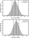Fig. B.1. Histograms showing the result of the Monte-Carlo analysis with the asymptotic formulation.

To propagate the observational uncertainties of the mixed-mode parameters into the inferred rotational components, we performed a Monte-Carlo analysis with N = 10, 000 realisations. For each realisation, we randomly drew the parameters (ν_a, ν_b, ΔΠ₂, ζ_a, ζ_b) from independent Gaussian distributions centred on the value reported in Deheuvels et al. (2017) and with their respective uncertainties. For every random draw, we then minimised the χ² difference between the observed multiplet frequencies and the model frequencies computed following Sect. 2.3.2, treating Ω_core and Ω_env as free parameters. The optimisation was carried out using the L-BFGS-B algorithm, with the bounds ν_c ∈ [0, 1] μHz and ν_env ∈ [0, 0.1] μHz. Only successful minimisations were retained in the final sample. The resulting posterior distributions of ν_c and ν_env were summarised by their median values and their 16th–84th percentile ranges, which we report as our final uncertainties.

Appendix C: Bayesian priors

C.1. Priors on pressure mode and mixed ℓ = 1 modes parameters

The frequency of maximum power ν_max is fixed to the value given by PyA2Z, while we assign flat priors within ±5% of the initial guess for Δν and ΔΠ₁ to account for the uncertainties of the PyA2Z pipeline, and we chose not to constrain ε, as its value is highly sensitive to any change in Δν. We assigned the priors on δν_0, ℓ around the values predicted by scaling relations provided by Mosser et al. (2018), Corsaro et al. (2012). We assigned to q₁ a flat prior between 0.15 and 0.4 based on the results of previous studies such as Mosser et al. (2017a), Kuszlewicz et al. (2023).

For ε_g, 1, we chose a very uninformative flat prior between 0 and 1. In the same fashion we chose very uninformative flat priors for β_0, ℓ and α between −0.1 and 0.1. This range seemed appropriate as the α and β_0, ℓ parameters found by Appourchaux (2020) and Lund et al. (2017) in the same evolutionary stage were under 10⁻². We assigned flat priors for rotation rates, with values ranging from 0 to 1,000 nHz for the core and 0 to 100 nHz for the envelope. These core rotation prior was derived from the work of Deheuvels et al. (2017) for KIC 7341231 and informed by a visual inspection of the splittings observed in KIC 8179973. For the envelope rotation, we again utilised the Deheuvels et al. (2017) article for KIC 7341231, and assumed a core envelope contrast of at least 10 in KIC 8179973. All of those priors are summarised in table C.1.

C.2. Priors on KIC 7341231

A global analysis using PyA2Z gives Δν, ν_max, and a guess value of ΔΠ₁ using the stretched period method. The priors on those parameters were then chosen according to Sect. C.1. Refined values of ΔΠ₁ and Δν are obtained by fitting the mixed ℓ = 1 modes according to the method described in Sect. 3.2.7. Because the angle of inclination is high, we had access to the m = 0 components of each quintuplet. Hence, we decided to use the method described in 3.2.4 to constrain q₂. To use this method, we needed to access the following parameters and their associated uncertainties: ΔΠ₂, Δν, ν_a, ν_b and the position of the ℓ = 2 p mode that is given by ν₀ − δν_0, 2. Where ν_a and ν_b are the positions of the m = 0 components of each multiplet and ν₀ is the frequency of the closest radial mode. ΔΠ₂ and its associated uncertainty was then obtained following Sect. 3.2.2. In order to obtain δν_0, 2, we fitted a bimodal Gaussian model to the averaged collapse of the echelle diagram. We obtained δν_0, 2/Δν = 0.120 ± 0.002. We finally peakbagged ν_a, ν_b and ν₀ and obtained ν_a = 380.382 ± 0.023 μHz, ν_b = 382.627 ± 0.01 μHz, and ν₀ = 384.514 ± 0.011 μHz. Using those values and their uncertainties, we can use a Monte-Carlo method to sample the distribution of q₂ according to equation (42). We obtained q₂ = 0.041 ± 0.003. We decided to use a uniform prior on q₂ within 3 sigma of the obtained value.

Furthermore, since we are only interested in reproducing the frequencies of the star’s modes and an angle of inclination was already fitted by Deheuvels et al. (2012), we adopt a fixed angle of inclination of 85°, in order to limit the number of free parameters.

C.3. Priors on KIC 8179973

A global analysis using PyA2Z gives Δν, ν_max, and a guess value of ΔΠ₁ using the stretched period method. The priors on those parameters were then chosen according to Sect. C.1. Refined values of ΔΠ₁, Δν and a value of q₁ are obtained by fitting the mixed ℓ = 1 modes according to the method described in Sect. 3.2.7. In KIC 8179973, the angle of inclination is such that the m = 0 modes of the ℓ = 2 quintuplet are either absent or buried in the noise of the star. Hence, we cannot use the same method as the on used for KIC 7341231 to constrain q₂. However, we can still use simple analytical arguments to put a rough upper bound on q₂ as a function of q₁.

q₁ in itself is obtained by fitting the mixed ℓ = 1 modes according to the method described in Sect. 3.2.7. We obtain q₁ = 0.197 ± 0.001 which yields that q₂ < 0.107 using the arguments presented in Sect. 3.2.5. We use a uniform prior for the orientation of axis of rotation of the star with respect to the line of sight. This translates to a prior ∝sin(θ_inc) for θ_inc between 0° and 90°.

C.4. Corner plots and comparison data-model

We compared the frequencies obtained within our asymptotic Bayesian framework to the frequencies obtained by Deheuvels et al. 2012, 2017 using a peakbagging code. Both the asymptotic model and the peakbagged frequencies agree, particularly around the central frequency (ν_max) as can be seen on figure C.1. This congruence is expected, as the asymptotic approximation becomes less precise further from ν_max due to increasing sensitivity to surface effects. Crucially, the physically informed nature of our method allows it to account for small excesses of power that are often indistinguishable from noise in standard peakbagging procedures.

Fig. C.1. Echelle diagram comparing the oscillation frequencies derived from the Bayesian asymptotic model (circles, this work) with the peakbagged frequencies of KIC 7341231 (squares, Deheuvels et al. 2012, 2017, referred to as Dh12 in the legend of the figure). The markers for the model frequencies are rendered semi-transparent when the separation from a peakbagged frequency exceeds 1 μHz.

Fig. C.2. Corner plot of the Bayesian fit of all the parameters for KIC 7341231 (first part).

Fig. C.3. Corner plot of the Bayesian fit of all the parameters for KIC 7341231 (second part).

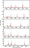Fig. C.4. Echelle diagram showing the superimposed data and asymptotic model for the most prominent modes of KIC 7341231.

Fig. C.5. Corner plot of the Bayesian fit of all the parameters for KIC 8179973 (first part).

Fig. C.6. Corner plot of the Bayesian fit of all the parameters for KIC 8179973 (second part).

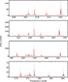Fig. C.7. Echelle diagram showing the superimposed data and asymptotic model for the most prominent modes of KIC 8179973.

All Tables

All Figures

Fig. 1. Illustration of the effect of near degeneracy on two coupled ℓ = 2 multiplets as the core rotation rate νc = Ωcore/2π increases for a fixed inclination angle of i = 42°. Each horizontally modelled PSD shows the combined visibility profile of the ten components (two sets of m = −2, −1, 0, +1, +2 modes) at a given νc. The greyscale background indicates how the multiplet structure evolves continuously with rotation.

In the text

Fig. 2. Asymptotic fit of KIC 7341231. In both panels, the Kepler data are in grey, and our asymptotic fit is in red. The radial, ℓ = 1, and ℓ = 2 modes are highlighted by the shading in green, blue, and yellow, respectively. Panel a: Two orders showing mixed ℓ = 2 modes with asymmetric splittings. Panel b: Zoom near 411 μHz on split ℓ = 2 modes. The m = 0, ±1, and ±2 components are marked in yellow, orange, and red. Panel c: Zoom near 381 μHz on split ℓ = 2 modes. The model is shown with thick red lins, data are in grey. The m = 0, ±1, and ±2 components of the ℓ = 2 mode are marked in yellow, orange, and red, and the m = ±1 components of the ℓ = 1 mode are marked in dark blue.

In the text

Fig. 3. Asymptotic fit of KIC 8179973. In both panels, the Kepler data are in grey, and our asymptotic fit is in red. The radial, ℓ = 1, and ℓ = 2 modes are highlighted by the shading in green, blue, and yellow, respectively. Panel a: Two orders showing mixed ℓ = 2 modes with asymmetric splittings. Panel b: Zoom near 352 μHz on split near-degenerate ℓ = 2 modes. The quadrupolar mixed m = 0, ±1, and ±2 components are marked in yellow, orange, and red, respectively. The full fit can be found in Fig. C.7.

In the text

	Fig. B.1. Histograms showing the result of the Monte-Carlo analysis with the asymptotic formulation.
In the text

	Fig. C.1. Echelle diagram comparing the oscillation frequencies derived from the Bayesian asymptotic model (circles, this work) with the peakbagged frequencies of KIC 7341231 (squares, Deheuvels et al. 2012, 2017, referred to as Dh12 in the legend of the figure). The markers for the model frequencies are rendered semi-transparent when the separation from a peakbagged frequency exceeds 1 μHz.
In the text

	Fig. C.2. Corner plot of the Bayesian fit of all the parameters for KIC 7341231 (first part).
In the text

	Fig. C.3. Corner plot of the Bayesian fit of all the parameters for KIC 7341231 (second part).
In the text

	Fig. C.4. Echelle diagram showing the superimposed data and asymptotic model for the most prominent modes of KIC 7341231.
In the text

	Fig. C.5. Corner plot of the Bayesian fit of all the parameters for KIC 8179973 (first part).
In the text

	Fig. C.6. Corner plot of the Bayesian fit of all the parameters for KIC 8179973 (second part).
In the text

	Fig. C.7. Echelle diagram showing the superimposed data and asymptotic model for the most prominent modes of KIC 8179973.
In the text

References

- Aerts, C., Christensen-Dalsgaard, J., & Kurtz, D. W. 2010, Asteroseismology (Springer Science+Business Media B.V.) [Google Scholar]
- Ahlborn, F., Joel Ong, J. M., Van Beeck, J., et al. 2025, A&A, 704, A230 [NASA ADS] [CrossRef] [EDP Sciences] [Google Scholar]
- Appourchaux, T. 2020, A&A, 642, A226 [NASA ADS] [CrossRef] [EDP Sciences] [Google Scholar]
- Astropy Collaboration (Robitaille, T. P., et al.) 2013, A&A, 558, A33 [NASA ADS] [CrossRef] [EDP Sciences] [Google Scholar]
- Astropy Collaboration (Price-Whelan, A. M., et al.) 2018, AJ, 156, 123 [Google Scholar]
- Basu, S., & Chaplin, W. J. 2017, Asteroseismic Data Analysis: Foundations and Techniques, Princeton Series in Modern Observational Astronomy (Princeton: Princeton University Press) [Google Scholar]
- Beck, P. G., Bedding, T. R., Mosser, B., et al. 2011, Science, 332, 205 [Google Scholar]
- Belkacem, K., Marques, J. P., Goupil, M. J., et al. 2015, A&A, 579, A30 [NASA ADS] [CrossRef] [EDP Sciences] [Google Scholar]
- Benomar, O., Bedding, T. R., Mosser, B., et al. 2013, ApJ, 767, 158 [Google Scholar]
- Bhattacharya, S., Das, S. B., Bugnet, L., Panda, S., & Hanasoge, S. M. 2024, ApJ, 970, 42 [NASA ADS] [CrossRef] [Google Scholar]
- Bordadágua, B., Ahlborn, F., Coppée, Q., et al. 2025, A&A, 699, A310 [NASA ADS] [CrossRef] [EDP Sciences] [Google Scholar]
- Borucki, W. J., Koch, D., Basri, G., et al. 2010, Science, 327, 977 [Google Scholar]
- Breton, S. N., García, R. A., Ballot, J., Delsanti, V., & Salabert, D. 2022, A&A, 663, A118 [NASA ADS] [CrossRef] [EDP Sciences] [Google Scholar]
- Bugnet, L. 2022, A&A, 667, A68 [NASA ADS] [CrossRef] [EDP Sciences] [Google Scholar]
- Bugnet, L., Prat, V., Mathis, S., et al. 2021, A&A, 650, A53 [NASA ADS] [CrossRef] [EDP Sciences] [Google Scholar]
- Ceillier, T., Eggenberger, P., García, R. A., & Mathis, S. 2013, A&A, 555, A54 [NASA ADS] [CrossRef] [EDP Sciences] [Google Scholar]
- Corsaro, E., Stello, D., Huber, D., et al. 2012, ApJ, 757, 190 [Google Scholar]
- Dalcin, L. D., Paz, R. R., Kler, P. A., & Cosimo, A. 2011, Adv. Water Resour., 34, 1124 [NASA ADS] [CrossRef] [Google Scholar]
- Das, S. B., Einramhof, L., & Bugnet, L. 2024, A&A, 690, A217 [NASA ADS] [CrossRef] [EDP Sciences] [Google Scholar]
- Decressin, T., Mathis, S., Palacios, A., et al. 2009, A&A, 495, 271 [NASA ADS] [CrossRef] [EDP Sciences] [Google Scholar]
- Deheuvels, S., García, R. A., Chaplin, W. J., et al. 2012, ApJ, 756, 19 [Google Scholar]
- Deheuvels, S., Doğan, G., Goupil, M. J., et al. 2014, A&A, 564, A27 [NASA ADS] [CrossRef] [EDP Sciences] [Google Scholar]
- Deheuvels, S., Ballot, J., Beck, P. G., et al. 2015, A&A, 580, A96 [NASA ADS] [CrossRef] [EDP Sciences] [Google Scholar]
- Deheuvels, S., Ouazzani, R. M., & Basu, S. 2017, A&A, 605, A75 [NASA ADS] [CrossRef] [EDP Sciences] [Google Scholar]
- Deheuvels, S., Li, G., Ballot, J., & Lignières, F. 2023, A&A, 670, L16 [NASA ADS] [CrossRef] [EDP Sciences] [Google Scholar]
- Di Mauro, M. P., Ventura, R., Cardini, D., et al. 2016, ApJ, 817, 65 [NASA ADS] [CrossRef] [Google Scholar]
- Dupret, M., Belkacem, K., Samadi, R., et al. 2009, A&A, 506, 57 [NASA ADS] [CrossRef] [EDP Sciences] [Google Scholar]
- Dziembowski, W. A., & Goode, P. R. 1992, ApJ, 394, 670 [Google Scholar]
- Eggenberger, P., Montalbán, J., & Miglio, A. 2012, A&A, 544, L4 [NASA ADS] [CrossRef] [EDP Sciences] [Google Scholar]
- Eggenberger, P., Lagarde, N., Miglio, A., et al. 2017, A&A, 599, A18 [CrossRef] [EDP Sciences] [Google Scholar]
- Eggenberger, P., den Hartogh, J. W., Buldgen, G., et al. 2019, A&A, 631, L6 [NASA ADS] [CrossRef] [EDP Sciences] [Google Scholar]
- Elsworth, Y., Howe, R., Isaak, G. R., McLeod, C. P., & New, R. 1990, Nature, 345, 322 [NASA ADS] [CrossRef] [Google Scholar]
- Fletcher, S. T., Chaplin, W. J., Elsworth, Y., Schou, J., & Buzasi, D. 2006, MNRAS, 371, 935 [NASA ADS] [CrossRef] [Google Scholar]
- Foreman-Mackey, D., Hogg, D. W., Lang, D., & Goodman, J. 2013, PASP, 125, 306 [Google Scholar]
- Foreman-Mackey, D., Agol, E., Ambikasaran, S., & Angus, R. 2017, AJ, 154, 220 [Google Scholar]
- Fuller, J., Lecoanet, D., Cantiello, M., & Brown, B. 2014, ApJ, 796, 17 [Google Scholar]
- Fuller, J., Cantiello, M., Stello, D., Garcia, R. A., & Bildsten, L. 2015, Science, 350, 423 [Google Scholar]
- Fuller, J., Piro, A. L., & Jermyn, A. S. 2019, MNRAS, 485, 3661 [NASA ADS] [Google Scholar]
- García, R. A., Hekker, S., Stello, D., et al. 2011, MNRAS, 414, L6 [NASA ADS] [CrossRef] [Google Scholar]
- García, R. A., Mathur, S., Pires, S., et al. 2014, A&A, 568, A10 [Google Scholar]
- García, R. A., Palakkatharappil, D. B., Bugnet, L., et al. 2024, 8th TESS/15th Kepler Asteroseismic Science Consortium Workshop, 123 [Google Scholar]
- Gehan, C., Mosser, B., Michel, E., Samadi, R., & Kallinger, T. 2018, A&A, 616, A24 [NASA ADS] [CrossRef] [EDP Sciences] [Google Scholar]
- Gizon, L., & Solanki, S. K. 2003, ApJ, 589, 1009 [Google Scholar]
- Gomes, P., & Lopes, I. 2020, MNRAS, 496, 620 [NASA ADS] [CrossRef] [Google Scholar]
- Gouhier, B., Jouve, L., & Lignières, F. 2022, A&A, 661, A119 [NASA ADS] [CrossRef] [EDP Sciences] [Google Scholar]
- Goupil, M. J., Mosser, B., Marques, J. P., et al. 2013, A&A, 549, A75 [NASA ADS] [CrossRef] [EDP Sciences] [Google Scholar]
- Goupil, M. J., Catala, C., Samadi, R., et al. 2024, A&A, 683, A78 [NASA ADS] [CrossRef] [EDP Sciences] [Google Scholar]
- Grosjean, M., Dupret, M.-A., Belkacem, K., et al. 2014, A&A, 572, A11 [CrossRef] [EDP Sciences] [Google Scholar]
- Harris, C. R., Millman, K. J., van der Walt, S. J., et al. 2020, Nature, 585, 357 [NASA ADS] [CrossRef] [Google Scholar]
- Hatt, E. J., Ong, J. M. J., Nielsen, M. B., et al. 2024, MNRAS, 534, 1060 [NASA ADS] [CrossRef] [Google Scholar]
- Hekker, S., & Christensen-Dalsgaard, J. 2017, A&ARv, 25, 1 [Google Scholar]
- Hernandez, V., Roman, J. E., & Vidal, V. 2005, ACM Trans. Math. Softw., 31, 351 [CrossRef] [Google Scholar]
- Hunter, J. D. 2007, Comput. Sci. Eng., 9, 90 [NASA ADS] [CrossRef] [Google Scholar]
- Jeffreys, H. 1925, Proc. London Math. Soc., S2–23, 428 [Google Scholar]
- Kallinger, T., De Ridder, J., Hekker, S., et al. 2014, A&A, 570, A41 [NASA ADS] [CrossRef] [EDP Sciences] [Google Scholar]
- Kuszlewicz, J. S., Chaplin, W. J., North, T. S. H., et al. 2019, MNRAS, 488, 572 [Google Scholar]
- Kuszlewicz, J. S., Hon, M., & Huber, D. 2023, ApJ, 954, 152 [NASA ADS] [CrossRef] [Google Scholar]
- Li, G., Deheuvels, S., Ballot, J., & Lignières, F. 2022, Nature, 610, 43 [NASA ADS] [CrossRef] [Google Scholar]
- Li, G., Deheuvels, S., Li, T., Ballot, J., & Lignières, F. 2023, A&A, 680, A26 [NASA ADS] [CrossRef] [EDP Sciences] [Google Scholar]
- Li, G., Deheuvels, S., & Ballot, J. 2024, A&A, 688, A184 [NASA ADS] [CrossRef] [EDP Sciences] [Google Scholar]
- Liagre, B., García, R. A., Mathur, S., et al. 2025, A&A, 702, A144 [NASA ADS] [CrossRef] [EDP Sciences] [Google Scholar]
- Loi, S. T. 2020a, MNRAS, 493, 5726 [CrossRef] [Google Scholar]
- Loi, S. T. 2020b, MNRAS, 496, 3829 [Google Scholar]
- Lund, M. N., Silva Aguirre, V., Davies, G. R., et al. 2017, ApJ, 835, 172 [Google Scholar]
- Lynden-Bell, D., & Ostriker, J. P. 1967, MNRAS, 136, 293 [Google Scholar]
- Maeder, A., & Zahn, J.-P. 1998, A&A, 334, 1000 [NASA ADS] [Google Scholar]
- Marques, J. P., Goupil, M. J., Lebreton, Y., et al. 2013, A&A, 549, A74 [NASA ADS] [CrossRef] [EDP Sciences] [Google Scholar]
- Mathis, S., & Bugnet, L. 2023, A&A, 676, L9 [NASA ADS] [CrossRef] [EDP Sciences] [Google Scholar]
- Mathis, S., & Zahn, J.-P. 2004, A&A, 425, 229 [NASA ADS] [CrossRef] [EDP Sciences] [Google Scholar]
- Mathis, S., Bugnet, L., Prat, V., et al. 2021, A&A, 647, A122 [EDP Sciences] [Google Scholar]
- Mathur, S., García, R. A., Régulo, C., et al. 2010, A&A, 511, A46 [NASA ADS] [CrossRef] [EDP Sciences] [Google Scholar]
- Meduri, D. G., Jouve, L., & Lignières, F. 2024, A&A, 683, A12 [NASA ADS] [CrossRef] [EDP Sciences] [Google Scholar]
- Mestel, L., & Weiss, N. O. 1987, MNRAS, 226, 123 [Google Scholar]
- Morel, P. 1997, A&AS, 124, 597 [NASA ADS] [CrossRef] [EDP Sciences] [Google Scholar]
- Mosser, B., Belkacem, K., Goupil, M. J., et al. 2011, A&A, 525, L9 [CrossRef] [EDP Sciences] [Google Scholar]
- Mosser, B., Goupil, M. J., Belkacem, K., et al. 2012a, A&A, 548, A10 [NASA ADS] [CrossRef] [EDP Sciences] [Google Scholar]
- Mosser, B., Elsworth, Y., Hekker, S., et al. 2012b, A&A, 537, A30 [NASA ADS] [CrossRef] [EDP Sciences] [Google Scholar]
- Mosser, B., Vrard, M., Belkacem, K., Deheuvels, S., & Goupil, M. J. 2015, A&A, 584, A50 [NASA ADS] [CrossRef] [EDP Sciences] [Google Scholar]
- Mosser, B., Pinçon, C., Belkacem, K., Takata, M., & Vrard, M. 2017a, A&A, 600, A1 [NASA ADS] [CrossRef] [EDP Sciences] [Google Scholar]
- Mosser, B., Belkacem, K., Pinçon, C., et al. 2017b, A&A, 598, A62 [NASA ADS] [CrossRef] [EDP Sciences] [Google Scholar]
- Mosser, B., Gehan, C., Belkacem, K., et al. 2018, A&A, 618, A109 [NASA ADS] [CrossRef] [EDP Sciences] [Google Scholar]
- Moyano, F. D., Eggenberger, P., Salmon, S. J. A. J., Mombarg, J. S. G., & Ekström, S. 2023, A&A, 677, A6 [NASA ADS] [CrossRef] [EDP Sciences] [Google Scholar]
- Müller, J., Coppée, Q., & Hekker, S. 2025, A&A, 696, A134 [NASA ADS] [CrossRef] [EDP Sciences] [Google Scholar]
- Ong, J. M. J., & Gehan, C. 2023, ApJ, 946, 92 [CrossRef] [Google Scholar]
- Ong, J. M. J., Bugnet, L., & Basu, S. 2022, ApJ, 940, 18 [NASA ADS] [CrossRef] [Google Scholar]
- O’Sullivan, N. K., & Aigrain, S. 2024, MNRAS, 531, 4181 [Google Scholar]
- Pereira, F., Campante, T. L., Cunha, M. S., et al. 2019, MNRAS, 489, 5764 [NASA ADS] [CrossRef] [Google Scholar]
- Pinçon, C., Belkacem, K., Goupil, M. J., & Marques, J. P. 2017, A&A, 605, A31 [NASA ADS] [CrossRef] [EDP Sciences] [Google Scholar]
- Pires, S., Mathur, S., García, R. A., et al. 2015, A&A, 574, A18 [NASA ADS] [CrossRef] [EDP Sciences] [Google Scholar]
- Rauer, H., Catala, C., Aerts, C., et al. 2014, Exp. Astron., 38, 249 [Google Scholar]
- Ricker, G. R., Winn, J. N., Vanderspek, R., et al. 2014, SPIE Conf. Ser., 9143, 20 [Google Scholar]
- Rogers, T. M., & Ratnasingam, R. P. 2025, ApJ, 983, L38 [Google Scholar]
- Schatzman, E. 1993, A&A, 279, 431 [NASA ADS] [Google Scholar]
- Schwarz, G. 1978, Ann. Stat., 6, 461 [Google Scholar]
- Shibahashi, H. 1979, PASJ, 31, 87 [NASA ADS] [Google Scholar]
- Skoutnev, V. A., & Beloborodov, A. M. 2025a, ApJ, 989, L4 [Google Scholar]
- Skoutnev, V. A., & Beloborodov, A. M. 2025b, ApJ, 988, 195 [Google Scholar]
- Spruit, H. C. 2002, A&A, 381, 923 [CrossRef] [EDP Sciences] [Google Scholar]
- Stello, D., Cantiello, M., Fuller, J., et al. 2016a, Nature, 529, 364 [Google Scholar]
- Stello, D., Cantiello, M., Fuller, J., Garcia, R. A., & Huber, D. 2016b, PASA, 33, e011 [Google Scholar]
- Takahashi, K., & Langer, N. 2021, A&A, 646, A19 [NASA ADS] [CrossRef] [EDP Sciences] [Google Scholar]
- Takata, M. 2016a, PASJ, 68, 91 [NASA ADS] [CrossRef] [Google Scholar]
- Takata, M. 2016b, PASJ, 68, 109 [NASA ADS] [CrossRef] [Google Scholar]
- Tassoul, M. 1980, ApJS, 43, 469 [Google Scholar]
- Tayler, R. J. 1973, MNRAS, 161, 365 [CrossRef] [Google Scholar]
- Toutain, T., & Appourchaux, T. 1994, A&A, 289, 649 [NASA ADS] [Google Scholar]
- Unno, W., Osaki, Y., Ando, H., Saio, H., & Shibahashi, H. 1989, Nonradial Oscillations of Stars (Berlin: Springer-Verlag) [Google Scholar]
- van Lier, T., Müller, J., & Hekker, S. 2025, A&A, 700, A1 [NASA ADS] [CrossRef] [EDP Sciences] [Google Scholar]
- Virtanen, P., Gommers, R., Oliphant, T. E., et al. 2020, Nat. Meth., 17, 261 [Google Scholar]
- Wentzel, G. 1926, Zeitschrift fur Physik, 38, 518 [Google Scholar]
- Woodard, M. F. 1984, Ph.D. Thesis, University of California, San Diego [Google Scholar]
- Zahn, J.-P. 1992, A&A, 265, 115 [NASA ADS] [Google Scholar]
- Zahn, J.-P., Brun, A. S., & Mathis, S. 2007, A&A, 474, 145 [NASA ADS] [CrossRef] [EDP Sciences] [Google Scholar]
This is possible because in the g-mode cavity,  , and hence the integral is a strictly increasing function of r. This change of variables leads to