| Issue |
A&A
Volume 707, March 2026
|
|
|---|---|---|
| Article Number | L6 | |
| Number of page(s) | 9 | |
| Section | Letters to the Editor | |
| DOI | https://doi.org/10.1051/0004-6361/202558051 | |
| Published online | 26 February 2026 | |
Letter to the Editor
Spectral variability of Phobos and Deimos from TGO/CaSSIS multiband observations
1
Centro di Studi Attività Spaziali – “Giuseppe Colombo” (CISAS/UniPD) Via Venezia 15 35131 Padova (PD), Italy
2
Istituto Nazionale di Astrofisica, Osservatorio Astronomico di Padova (INAF/OAPD), Vicolo dell’Osservatorio 5 35122 Padova (PD), Italy
3
Physikalisches Institut, University of Bern Sidlerstr. 5 CH-3012 Bern, Switzerland
4
INAF Osservatorio Astronomico di Arcetri largo E. Fermi n.5 I-50125 Firenze, Italy
5
Brown University, Department of Earth, Environmental and Planetary Sciences 180 Thayer St Providence RI 02912, USA
6
Institute for Earth and Space Exploration, University of Western Ontario, Dept. of Earth Sciences 1151 Richmond Street London Onatrio N6A 5B7, Canada
7
The SETI Institute, 339 Bernardo Ave Suite 200 Mountain View CA 94043, USA
8
School of Physical Sciences, The Open University Walton Hall Milton Keynes, UK
★ Corresponding authors: This email address is being protected from spambots. You need JavaScript enabled to view it.
; This email address is being protected from spambots. You need JavaScript enabled to view it.
Received:
10
November
2025
Accepted:
4
February
2026
Abstract
Aims. We present a comparative visible and near-infrared multiband analysis of Phobos and Deimos aimed at characterising the compositional variability of the Martian moons.
Methods. From multiband observations acquired by the Colour and Surface Stereo Imaging System (CaSSIS) on board on the ESA/ExoMars Trace Gas Orbiter (TGO), we analysed spectral ratios tracing ferric and ferrous minerals and mapped them over the surfaces of the Martian moons. We identified regions of interest (ROIs) on both moons and compare their mean spectra and spectral slopes.
Results. We identified an overall similarity between the two Martian moons, whose variability can be explained by a different degree of ferric and ferrous mineralogy. In particular, the blue unit of Phobos can be explained by the presence of ferrous minerals, while the ferric minerals dominate in the red unit. We show that overall the Deimos surface matches the Phobos red units. On the contrary, the Deimos bright blue spots are spectrally similar to the Phobos transitional unit. We show the presence of a 1000 nm band only in the blue unit of Phobos.
Conclusions. Our comparative multiband analysis of Phobos and Deimos is consistent with a similar composition of the two Moons, suggested by the spectral similarity of their redder units. The detection of an absorption towards 1000 nm in the blue unit suggests an exogenous nature of the latter.
Key words: planets and satellites: composition / planets and satellites: general / planets and satellites: individual: Phobos / planets and satellites: individual: Deimos
© The Authors 2026
 Open Access article, published by EDP Sciences, under the terms of the Creative Commons Attribution License (https://creativecommons.org/licenses/by/4.0), which permits unrestricted use, distribution, and reproduction in any medium, provided the original work is properly cited.
This article is published in open access under the Subscribe to Open model. This email address is being protected from spambots. You need JavaScript enabled to view it. to support open access publication.
1. Introduction
Mars has two natural satellites, Phobos and Deimos, whose origin is still very debated (Pajola et al. 2012, 2013; Takir et al. 2022; Kuramoto et al. 2022). The two leading hypotheses are asteroid gravitational capture (Hansen 2018) and the impact scenario (Craddock 2011; Rosenblatt & Charnoz 2012; Canup & Salmon 2018; Hyodo et al. 2018). Murchie et al. (1991) first divided the surface of Phobos into two main units, characterised by a distinctive Visible (Vis-channel with central wavelength λc = 480 nm) and Near Infrared (NIR, λc = 940 nm), as shown in Fig. A.1 (Thomas et al. 2011; Pajola et al. 2018). The red unit extends over the majority of its surface, characterised by a relatively steep Vis-NIR slope spectrum and it is thought to consist of old and deeply space-weathered material (Murchie & Erard 1996; Basilevsky et al. 2014; Munaretto et al. 2025). On the contrary, the blue unit has a much flatter spectrum and it is geographically associated with the 9 km crater Stickney, extending as far as 5 km from its eastern rim (Thomas et al. 2011; Basilevsky et al. 2014). This unit likely consists of a ≤100 m thick layer (Thomas et al. 2011) and its origin is an open question. The leading hypotheses are that it formed from material either ejected during the Stickney crater emplacement (Murchie et al. 1991; Murchie & Erard 1996), or was deposited by an exogenous source, i.e. non-indigenous to Phobos (Basilevsky et al. 2014; Munaretto et al. 2025). Eventually, a third “transitional” Phobos unit, characterised by a mixture between the blue and the red units and showing an intermediate spectral slope was identified (Murchie et al. 1991; Pajola et al. 2025). Vis-NIR spectral data of both Phobos and Deimos lack evident diagnostic absorption features, except for a possible 650 nm band detected in Mars Pathfinder data by Murchie et al. (1999) and in data from the Compact Reconnaissance Imaging Spectrometer for Mars (CRISM, Murchie et al. 2007) on their red units by Fraeman et al. (2014) and attributed to either desiccated nontronite, space-weathered, anhydrous silicates or ferric minerals such as hematite and goethite (Clark 2004). In addition, data from the Video Spectrometric System (VSK) (Avanesov et al. 1989) and Imaging Spectrometer for Mars (ISM) (Bibring et al. 1989) on the Phobos 2 mission (Murchie & Erard 1996; Gendrin et al. 2005) and from the Hubble Space Telescope (HST, Cantor et al. 1999) revealed a weak feature around 1000–1040 nm in the red unit of Phobos. More recently, Pajola et al. (2025) tentatively detected a similar reflectance decrease in Observatoire pour la Minéralogie, l’Eau, les Glaces et l’Activité (Mars Express/OMEGA) dataset covering Phobos’ blue unit. The study of the spectra of the Martian moons and their variability is crucial for assessing the current physical state of their surfaces, as well as their composition. High-resolution spectroscopic and/or multifilter analyses that are sensitive to these features are therefore of great value for improving our understanding of the overall spectral variability of the Mars system. In this context, valuable observations have been recently acquired by the Colour and Stereo Surface Imaging System (CaSSIS, Thomas et al. 2017) on board the ESA ExoMars Trace Gas Orbiter (TGO) mission. In addition to its stereo capabilities, CaSSIS acquires images at four different central wavelengths (see Table F.1 for further details): 499.9 nm (BLU), 675.0 nm (PAN), 836.2 nm (RED), and 936.7 nm (NIR) with good photometric accuracy for Vis-NIR compositional studies (Thomas et al. 2022). CaSSIS is highly sensitive to capture the absorption at 1000 nm and 500–700 nm, due to the presence of ferrous (i.e. Fe2+) and ferric (i.e. Fe3+) bearing minerals, as shown by Tornabene et al. (2018). The occurrence of these two different mineralogies can be identified through specific CaSSIS band ratios; in particular, the PAN/BLU and RED/PAN ratios are a proxy for ferric minerals, such as hematite and goethite. Other possibilities that could mimic the spectral signature of ferric mineralogy are (i) the space weathering (SW) products (e.g. Fe-nanophase minerals produced by H+ ions and/or micrometeorite impacts; Pieters et al. 2000; Sasaki et al. 2001) and (ii) desiccated phyllosilicates, such as nontronite showing similar features (Fraeman et al. 2014). Finally, the PAN/NIR ratio traces the absorption at 1000 nm, due to the electronic transition of the Fe2+ that occurs in ferrous mafic minerals, such as olivine and pyroxene (Tornabene et al. 2018). This band depth commonly decreases because of SW (Wargnier et al. 2023).
In this work we present a comparative multifilter analysis of CaSSIS observations of Phobos and Deimos aiming at investigating and providing their spectral variability and insights on the surface physical condition.
2. Methods
We selected four CaSSIS observations of Phobos covering the blue, the red, and the transitional unit, and one observation of Deimos (see Table E.1 for images deatils). As previously done for Phobos (i.e. Pajola et al. 2018; Fornasier et al. 2024), we photometrically corrected with the Lommel-Seeliger disk function (LS). Each pixel local incidence (i) and emission (e) angle required as inputs for the LS correction, were computed alongside longitude and latitude using the SpiceyPy library (Annex et al. 2020) and the NAIF SPICE kernels (Acton 1996; Stooke & Pajola 2019) with the Gaskell (2020) and Ernst et al. (2023) shape models for Phobos and Deimos, respectively. Examples of local incidence, emission, and phase maps are presented in Fig. B.1. The observation images were taken through multiple exposures (framelets), with the target moving across the focal plane and passing through each filter’s field of view. From these, a multispectral datacube was generated by coregistering the BLU, RED, and NIR framelets to the PAN using the Elastix library (Klein et al. 2009). In addition, the geometry backplanes (incidence, emission, phase, latitude, and longitude) showed a slight misalignment with respect to the corresponding acquired image. To correct for this, we aligned them to the PAN using a rigid transformation. For each datacube, an RGB colour composite image was prepared (see Fig. 1A,B), along with the PAN/NIR, PAN/BLU, and RED/PAN band ratios following Tornabene et al. (2018), which have been merged into a single map-projected mosaic (Fig. 2). To accurately identify the pixels whose spectra exhibit a dip around 1000 nm, we computed NIR/PAN and NIR/RED ratios, shown in Figs. 3, D.2 as a percentage of band depth using the following formula: BD = (1 − BandRatio)⋅100.
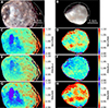 |
Fig. 1. CaSSIS RGB (RED = RED, G = PAN, B = BLU) colour composite with latitude–longitude grids of Phobos (A) and Deimos (B), RED/PAN (C,D), PAN/BLU (E,F), PAN/NIR (G,H) for Phobos (cube 296, left) and Deimos (cube 229, right). The band ratios have been normalised with the same factor, i.e. the mean of Phobos’ band ratio. The normalisation factors are 1.1327 for RED/PAN, 1.0899 for PAN/BLU, and 0.8683 for PAN/NIR. |
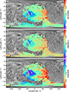 |
Fig. 2. Equirectangular maps projection showing the distribution of RED/PAN (A), PAN/BLU (B), and PAN/NIR (C) on the surface of Phobos, overlain on the Viking mosaic (Simonelli et al. 1993). Emission angles above 60° are filtered. |
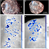 |
Fig. 3. Derived 1000 nm band depth (in %) for cube 296 (left) and cube 320-1 (right). The pixels showing the feature are clustered in the Phobos blue unit. |
3. Results
As outlined in Fig. 1C,F and Fig. 2A,B, RED/PAN and PAN/BLU are higher in regions located in the red unit of Phobos. One possible explanation is that the red unit may be characterised by more space-weathered, and hence older, material with respect to the blue unit. On the contrary, the PAN/NIR ratio increases within the Phobos’ blue unit and, in line with its lower spectral slope, as reported in Pajola et al. (2025) and Munaretto et al. (2025), peaking closer to the eastern rim of Stickney (see Figs. 1G, 2C). In Fig. 1H the Deimos PAN/NIR show higher values in the bright spots visible in the RGB colour composite (see Fig. 1B). This confirms the result from multiband photometry obtained on HRSC data (Wargnier et al. 2025). Focusing on the PAN/NIR ratio, we selected specific regions of interest (ROIs) (see Fig. C.1) and computed their mean spectra (Fig. 4) in order to study the ratio variability across the surface. The obtained set of spectra are clustered in three main groups: (i) spectra that present a flat trend and a downward dip towards 1000 nm, suggesting an absorption band, i.e. Pb1-6; (ii) spectra with a higher slope, i.e. Dr1-Pr1-2, no dip towards 1000 nm, and a possible absorption between 600 nm and 800 nm; (iii) spectra that are intermediate between (i) and (ii), i.e. Dt1-2 and Pt1-2. The spatial distribution of pixels that show a downward deflection towards the NIR is shown in Fig. 3, Fig. D.1, and Fig. D.2 using the NIR/PAN and the NIR/RED ratios, with the latter being more sensitive than the former, given the generally red spectral slope of all spectra. Such a distribution is clearly clustered inside the blue unit, meaning that the lower reflectance in the NIR with respect to the PAN and RED is unlikely to be a calibration artefact. In addition, a very conservative estimate of the CaSSIS absolute calibration accuracy is 2.8% (Thomas et al. 2022), meaning that the ratios have a radiometric uncertainty of 3.9%, derived from error propagation. The robustness of the CaSSIS calibration was further confirmed by the comparison with a CRISM spectrum of the blue unit similar to the one analysed by Fraeman et al. (2014) (see Appendix G). The presence of several pixels above this threshold in the NIR/PAN (Figs. 3, D.1), especially in the NIR/RED (Fig. D.2), further supports the robust detection of a spectral feature near 1000 nm within the blue unit of Phobos. This interpretation is reinforced by the linear regression and limb analysis presented in Appendix H.
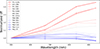 |
Fig. 4. Mean spectra normalised to BLU associated with ROIs in Fig. C.1. The error bars represent 1σ standard errors. The number of pixels of each ROI is reported in the legend. The spectra are labelled as Pbn, Prn, Ptn, and Dbn, where P and D denote Phobos and Deimos; b, r, and t refer to the blue, red, and transitional units; and n indicates the spectrum number. |
4. Discussion
By analysing diagnostic CaSSIS band ratios sensitive to ferrous (PAN/NIR), ferric, and SW (RED/BLU, PAN/BLU) mineralogy, we found that the blue unit of Phobos is consistent with a lower PAN/NIR, linked by Tornabene et al. (2018) to a ferrous mineralogy (Fig. 2A,B). On the contrary, the red unit is characterised by a higher RED/PAN and PAN/BLU, which is linked to a more ferric mineralogy (Tornabene et al. 2018). A similar trend is identified on the bright spots of Deimos, which correlate with a higher PAN/NIR, in contrast to the redder regions that display a higher RED/PAN and PAN/BLU. We further analysed this trend by comparing the spectra of the ROIs selected on the two moons’ spectral units (Fig. C.1). In particular, spectra from the Phobos blue unit (see Fig. C.1 C,H), consistently show a deflection towards 1000 nm. Since this downward dip is clustered around the blue unit (Figs. 3, D.1, D.2) and occurs at thresholds higher than the (conservative) radiometric accuracy of the data, both with respect to the RED and PAN filters, we argue that it can be attributed to the presence of a 1000 nm band of mafic minerals, such as olivine, to which CaSSIS is particularly sensitive (Tornabene et al. 2018). This confirms a previous tentative detection suggested by Pajola et al. (2025), while, as we detail in Appendix G, past non-detections by CRISM (Fraeman et al. 2014) can be attributed to the lower spatial resolution of the observations. On the contrary, the Phobos red and transitional units (including Stickney) do not show this band, but instead are possibly characterised by an absorption between 600–800 nm consistent with the presence of SW products (Fig. 4) (Fraeman et al. 2014). This indicates (i) a spectral variability and a different regolith maturity between Phobos blue and red/transitional units, in agreement with photometric studies (Munaretto et al. 2025), and (ii) supports an exogenous origin for the blue unit of Phobos. Deimos shows a similar variability to that of the Phobos red unit, the only difference being the lack of regions bearing a 1000 nm dip. This supports the fact that the regolith of the two moons have very similar physical and compositional properties, as found from spectrophotometric analyses (Fornasier et al. 2024; Wargnier et al. 2024; Munaretto et al. 2025). Nevertheless, it is worth highlighting that the bluest units of Deimos closely represent spectra of the Phobos transitional unit. This may suggest that the Phobos blue unit was also put in place on Deimos, but we do not observe a ferrous signature because it is masked by the lower spatial resolution of the observations and more significant mixing with the spectrally red surroudings.
5. Conclusions
We have analysed a set of CaSSIS images of Phobos and Deimos with the aim of investigating the variability of the Martian moon spectra. Our findings suggests the following:
-
Phobos’ spectral variability reflects higher PAN/NIR ratios in the blue unit and higher RED/PAN and PAN/BLU ratios in the red unit, likely due to variable ferrous-ferric mineralogy and possible SW.
-
This spectral variability also describes Deimos, in agreement with the similar spectrophotometric properties of the two moons (Munaretto et al. 2025; Wargnier et al. 2025).
-
The Phobos blue unit is characterised by a 1000 nm absorption, detected in this region for the first time, suggesting an exogenous origin.
-
The bright regions of Deimos are spectrally similar to the Phobos transitional unit, possibly suggesting the presence of Phobos blue unit material within Deimos bright spots.
Future data and samples will be returned by the Japanese space agency (JAXA) Martian Moons eXploration (MMX) (Kuramoto et al. 2022) mission, set to launch in late 2026. This new mission will shed further light on the origin of the Martian moons and their spectral units, thanks to the high-resolution data that will be acquired by the MMX Infrared Spectrometer (MIRS; Barucci et al. 2021) and the sample return programme, which is expected to bring samples back to Earth in 2031.
Acknowledgments
In memory of Riccardo Pozzobon: colleague, friend, and inspiration for young researchers, who left us far too soon. The authors are thankful to the anonymous Reviewer for the constructive suggestions, comments and corrections, that led to an important improvement of the paper. CaSSIS is a project of the University of Bern and funded through the Swiss Space Office via ESA’s PRODEX programme. The instrument hardware development was also supported by the Italian Space Agency (ASI) (ASI-INAF agreement no. 2020-17-HH.0), INAF/Astronomical Observatory of Padova, and the Space Research Center (CBK) in Warsaw. Support from SGF (Budapest), the University of Arizona (Lunar and Planetary Lab.) and NASA are also gratefully acknowledged. Operations support from the UK Space Agency under grant ST/R003025/1 is also acknowledged. We gratefully acknowledge support from the Italian Space Agency (ASI) with ASI-INAF agreements n. 2022-8-HH.0 and n. 2024-40-HH.0. LLT wishes to personally acknowledge funding and support from the Canadian NSERC Discovery Grant programme (RGPIN 2020-06418) and the Canadian Space Agency (CSA) Planetary and Astronomy Missions Co-Investigator (24EXPROSS1) programme.
References
- Acton, C. H., Jr. 1996, Planet. Space Sci., 44, 65 [CrossRef] [Google Scholar]
- Annex, A. M., Pearson, B., Seignovert, B., et al. 2020, J. Open Source Softw., 5, 2050 [CrossRef] [Google Scholar]
- Avanesov, G., Bonev, B., Kempe, F., et al. 1989, Nature, 341, 585 [Google Scholar]
- Barucci, M. A., Reess, J.-M., Bernardi, P., et al. 2021, Earth Planets Space, 73, 1 [CrossRef] [Google Scholar]
- Basilevsky, A., Lorenz, C., Shingareva, T., et al. 2014, Planet. Space Sci., 102, 95 [CrossRef] [Google Scholar]
- Bibring, J.-P., Combes, M., Langevin, Y., et al. 1989, Nature, 341, 591 [Google Scholar]
- Cantor, B. A., Wolff, M. J., Thomas, P. C., James, P. B., & Jensen, G. 1999, Icarus, 142, 414 [NASA ADS] [CrossRef] [Google Scholar]
- Canup, R., & Salmon, J. 2018, Sci. Adv., 4, eaar6887 [NASA ADS] [CrossRef] [Google Scholar]
- Clark, R. N. 2004, Chapeter 2. Spectroscopy of Rocks and Minerals, and Principles of Spectroscopy (Mineralogical Association of Canada), 17 [Google Scholar]
- Craddock, R. A. 2011, Icarus, 211, 1150 [NASA ADS] [CrossRef] [Google Scholar]
- Ernst, C. M., Daly, R. T., Gaskell, R. W., et al. 2023, Earth Planets Space, 75, 103 [NASA ADS] [CrossRef] [Google Scholar]
- Fornasier, S., Wargnier, A., Hasselmann, P. H., et al. 2024, A&A, 686, A203 [NASA ADS] [CrossRef] [EDP Sciences] [Google Scholar]
- Fraeman, A., Murchie, S., Arvidson, R., et al. 2014, Icarus, 229, 196 [NASA ADS] [CrossRef] [Google Scholar]
- Gaskell, R. W. 2020, Gaskell Phobos Shape Model V1.0, urn:nasa:pds:gaskell.phobos.shape-model::1.0 [Google Scholar]
- Gendrin, A., Langevin, Y., & Erard, S. 2005, JGR: Planets, 110, E4 [Google Scholar]
- Hansen, B. M. S. 2018, MNRAS, 475, 2452 [CrossRef] [Google Scholar]
- Hyodo, R., Genda, H., Charnoz, S., Pignatale, F. C., & Rosenblatt, P. 2018, ApJ, 860, 150 [Google Scholar]
- Klein, S., Staring, M., Murphy, K., Viergever, M. A., & Pluim, J. P. 2009, IEEE Trans. Med. Imaging, 29, 196 [Google Scholar]
- Kuramoto, K., Kawakatsu, Y., Fujimoto, M., et al. 2022, Earth Planets Space, 74, 12 [NASA ADS] [CrossRef] [Google Scholar]
- Munaretto, G., Pajola, M., Beccarelli, J., et al. 2025, A&A, 700, L1 [NASA ADS] [CrossRef] [EDP Sciences] [Google Scholar]
- Murchie, S., & Erard, S. 1996, Icarus, 123, 63 [CrossRef] [Google Scholar]
- Murchie, S. L., Britt, D. T., Head, J. W., et al. 1991, JGR: Solid Earth, 96, 5925 [Google Scholar]
- Murchie, S., Thomas, N., Britt, D., Herkenhoff, K., & Bell, J. F., III. 1999, JGR: Planets, 104, 9069 [Google Scholar]
- Murchie, S., Arvidson, R., Bedini, P., et al. 2007, JGR: Planets, 112, E5 [Google Scholar]
- Pajola, M., Lazzarin, M., Bertini, I., et al. 2012, MNRAS, 427, 3230 [NASA ADS] [CrossRef] [Google Scholar]
- Pajola, M., Lazzarin, M., Dalle Ore, C., et al. 2013, ApJ, 777, 127 [NASA ADS] [CrossRef] [Google Scholar]
- Pajola, M., Roush, T., Dalle Ore, C., Marzo, G. A., & Simioni, E. 2018, Planet. Space Sci., 154, 63 [NASA ADS] [CrossRef] [Google Scholar]
- Pajola, M., Beccarelli, J., Munaretto, G., et al. 2025, A&A, 697, A56 [NASA ADS] [CrossRef] [EDP Sciences] [Google Scholar]
- Pieters, C. M., Taylor, L. A., Noble, S. K., et al. 2000, Meteorit. Planet. Sci., 35, 1101 [CrossRef] [Google Scholar]
- Rosenblatt, P., & Charnoz, S. 2012, Icarus, 221, 806 [NASA ADS] [CrossRef] [Google Scholar]
- Sasaki, S., Nakamura, K., Hamabe, Y., Kurahashi, E., & Hiroi, T. 2001, Nature, 410, 555 [NASA ADS] [CrossRef] [Google Scholar]
- Simonelli, D. P., Thomas, P. C., Carcich, B. T., & Veverka, J. 1993, Icarus, 103, 49 [NASA ADS] [CrossRef] [Google Scholar]
- Stooke, P., & Pajola, M. 2019, Planetary Cartography and GIS (Springer), 191 [Google Scholar]
- Takir, D., Matsuoka, M., Waiters, A., Kaluna, H., & Usui, T. 2022, Icarus, 371, 114691 [NASA ADS] [CrossRef] [Google Scholar]
- Thomas, N., Stelter, R., Ivanov, A., et al. 2011, Planet. Space Sci., 59, 1281 [NASA ADS] [CrossRef] [Google Scholar]
- Thomas, N., Cremonese, G., Ziethe, R., et al. 2017, Space Sci. Rev., 212, 1897 [NASA ADS] [CrossRef] [Google Scholar]
- Thomas, N., Pommerol, A., Almeida, M., et al. 2022, Planet. Space Sci., 211, 105394 [NASA ADS] [CrossRef] [Google Scholar]
- Tornabene, L. L., Seelos, F. P., Pommerol, A., et al. 2018, Space Sci. Rev., 214, 1 [NASA ADS] [CrossRef] [Google Scholar]
- Wargnier, A., Poggiali, G., Doressoundiram, A., et al. 2023, MNRAS, 524, 3809 [NASA ADS] [CrossRef] [Google Scholar]
- Wargnier, A., Gautier, T., Doressoundiram, A., et al. 2024, Icarus, 421, 116216 [Google Scholar]
- Wargnier, A., Poggiali, G., Yumoto, K., et al. 2025, A&A, 694, A304 [NASA ADS] [CrossRef] [EDP Sciences] [Google Scholar]
Appendix A: Phobos’ Context
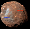 |
Fig. A.1. HiRISE image (PSP-007769-9010-IRB) of Phobos showing the largest crater on the surface (Stickney, white arrow), the blue unit covering the eastern rim of such crater, and the red unit dominating the surface of Phobos. |
Appendix B: Spectral ratio
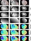 |
Fig. B.1. CaSSIS RGB colour composite, incidence, emission, phase, RED/PAN, PAN/BLU, and PAN/NIR for Phobos cubes 283 (left panels), 228 (central panels), and 320-1 (right panles). The normalisation factors are (1.1486, 1.1356, 1.1429) for RED/PAN, (1.1204, 1.0786, 1.0313) for PAN/BLU, and (0.8549, 0.8600, 0.8229) for PAN/NIR. |
Appendix C: ROIs selection
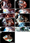 |
Fig. C.1. Location of Phobos ROIs on CaSSIS RGB (RED=RED, G=PAN, B=BLU) image composite for cube 296 (A, C, E), 320-1 (B, D), 228 (F, H, L), and 283 (G, I). Location of Deimos ROIs on CaSSIS cube 229 (M). |
Appendix D: The 1000 nm band
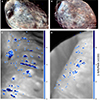 |
Fig. D.1. Derived 1000 nm band depth (in %) for cube 228 (left) and cube 283 (right). The pixel showing this feature are clustered in the Phobos blue unit. |
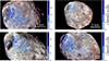 |
Fig. D.2. 1000 nm band depth (in %) has been calculated as in Figs. 3 and D.1, but using the NIR/RED ratio instead of NIR/PAN. In this case as well, the pixels cluster within the region identified by the blue unit. |
Appendix E: Observational parameters
Observing parameters of Phobos and Deimos with CaSSIS.
Appendix F: CaSSIS parameters
CaSSIS main parameters (Thomas et al. 2017).
Appendix G: Comparison with other datasets
In this section we provide a further assessment of the calibration of CaSSIS by comparing with spectra extracted from CRISM. To also investigate the effect of the different spatial resolution between CaSSIS and CRISM, we consider CRISM spectra from cube FRT2992 and a ROI of a similar size as the one used in Fraeman et al. (2014). We comapred a) the CRISM spectra extracted from this ROI and resampled to the CaSSIS wavelengths (green line in Fig. G.1D) with spectra extracted from the same ROI on b) the original CaSSIS dataset (orange line in Fig. G.1D) and c) after the convolution of the CaSSIS dataset for the CRISM PSF and resampling to the CRISM spatial resolution (light-blue line in Fig. G.1D). All spectra have been continuum-removed to factor out the absolute reflectance differences due to the different illumination and observation conditions. The resulting continuum-removed spectra (Fig. G.1D) are comparable both within their error-bars and within the 2.8% radiometric accuracy of CaSSIS, further validating the calibration of the instrument (Thomas et al. 2022). All these spectra do not show statistically significant dips towards the NIR filter. Instead, CaSSIS spectra extracted from much smaller Pb4 and Pb5 ROIs (that cannot be properly sampled in the much lower resolution CRISM dataset due to their small size) show a 1000 nm dip in the NIR which is well above the radiometric uncertainties. This analysis suggests that past studies of the blue unit with CRISM did not identify any 1000 nm spectral feature due to the low spatial resolution of the observation.
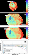 |
Fig. G.1. A) ROI identified on the CRISM FRT2992 PAN/NIR computed using as PAN the band at λ= 696 nm and for the NIR the band at λ = 938nm and similar in size to the one used in Fraeman et al. (2014), but optimised to enhance the 1000 nm absorption; B) ROI identified on the original Cassis PAN/NIR; C) ROI identified on the degraded Cassis PAN/NIR; D) Comparison between continuum removed mean spectra extracted from the ROI shown in panels A, B, and C, and panel D. In green, the CRISM spectrum resampled at the CaSSIS filter wavelengths. In black the original CRISM spectrum. In orange, the CaSSIS spectrum extracted from the original dataset. In light blue, the CaSSIS spectrum extracted from the dataset degraded to the CRISM spatial resolution (panel C). In pink and dark blue: CaSSIS spectra from ROIs Pb4 and Pb5. |
Appendix H: NIR PSF effect
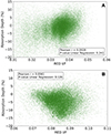 |
Fig. H.1. Absorption band depth (in %) plotted against the RED I/F value for each pixel in the stp296 dataset (A) and the stp320-1 dataset (B). No correlation is observed, as confirmed by both linear regression analysis and the Pearson correlation coefficient. |
If the 1000 nm feature observed and described in this work were caused by the broader point spread function (PSF) of the NIR filter, two main effects would be expected. First, a broader PSF would reduce the NIR I/F, artificially mimicking the presence of a 1000 nm absorption feature. This effect would be stronger for higher RED I/F values, thus implying a linear correlation between the RED I/F and the absorption depth of the 1000 nm band. To test this hypothesis, we computed the absorption depth in percentage for each pixel of the stp296 dataset and plotted it against the RED I/F (see Fig. H.1 A). As shown in Fig. H.1 A, the data points appear clustered and do not exhibit a clear correlation between the two quantities. Testing the null hypothesis (H0), namely that the slope is equal to zero, yields a p-value of 0.241. This result indicates that the slope is not statistically different from zero and, therefore, that there is no statistical evidence for a correlation between the pixel values and the presence of the absorption band. For completeness, we also computed the Pearson correlation coefficient r, a widely used statistical measure of linear correlation between two datasets. We obtained a Pearson r value of 0.0028, which confirms the result derived from the linear regression analysis. Since this effect, if present, would be expected to become more pronounced at higher pixel intensity values, we also extended the analysis to the stp320-1 cube, acquired at a phase angle close to 0 degrees, which exhibits the highest pixel values in the entire dataset. We first note that the I/F range of stp320-1 is significantly higher than that of the stp296 cube, and in particular that the red unit in stp320-1 is brighter than the blue unit in stp296. Therefore, if a correlation between increasing pixel brightness and the presence of the absorption band existed, this effect should be enhanced for this dataset. We applied the same procedure and obtained the results shown in Fig. H.1B. The linear regression yields a p-value of 0.126, while the Pearson correlation coefficient is r = 0.0061, confirming the absence of any statistically significant correlation between the presence of the absorption band and the pixel I/F. This analysis further confirms that no clear correlation exists between the RED I/F and the presence of the absorption band, supporting the interpretation that the band represents a real spectral feature of Phobos.
Another indication of a broader NIR PSF compared to the other filters would be a higher signal level beyond the Phobos limb. To test this hypothesis, we computed the I/F profiles across the limb and compared the NIR and RED brightness levels beyond the limb. In Fig. H.2a, we show two selected profiles (AA’ and BB’), noting that the same result is obtained for other profile orientations. The comparison is presented in Fig. H.2b. As can be seen, the NIR limb is not brighter than the RED limb; instead, the two profiles are highly consistent. This result indicates that the effect of the PSF is negligible.
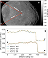 |
Fig. H.2. I/F profile analysis to study the NIR PSF effect. The selected I/F profiles (a), together with the corresponding plotted I/F profile (b) are plotted. The two profiles are consistent, and no brighter Phobos limb is observed in the NIR filter. |
All Tables
All Figures
|
Fig. 1. CaSSIS RGB (RED = RED, G = PAN, B = BLU) colour composite with latitude–longitude grids of Phobos (A) and Deimos (B), RED/PAN (C,D), PAN/BLU (E,F), PAN/NIR (G,H) for Phobos (cube 296, left) and Deimos (cube 229, right). The band ratios have been normalised with the same factor, i.e. the mean of Phobos’ band ratio. The normalisation factors are 1.1327 for RED/PAN, 1.0899 for PAN/BLU, and 0.8683 for PAN/NIR. |
| In the text | |
|
Fig. 2. Equirectangular maps projection showing the distribution of RED/PAN (A), PAN/BLU (B), and PAN/NIR (C) on the surface of Phobos, overlain on the Viking mosaic (Simonelli et al. 1993). Emission angles above 60° are filtered. |
| In the text | |
|
Fig. 3. Derived 1000 nm band depth (in %) for cube 296 (left) and cube 320-1 (right). The pixels showing the feature are clustered in the Phobos blue unit. |
| In the text | |
|
Fig. 4. Mean spectra normalised to BLU associated with ROIs in Fig. C.1. The error bars represent 1σ standard errors. The number of pixels of each ROI is reported in the legend. The spectra are labelled as Pbn, Prn, Ptn, and Dbn, where P and D denote Phobos and Deimos; b, r, and t refer to the blue, red, and transitional units; and n indicates the spectrum number. |
| In the text | |
|
Fig. A.1. HiRISE image (PSP-007769-9010-IRB) of Phobos showing the largest crater on the surface (Stickney, white arrow), the blue unit covering the eastern rim of such crater, and the red unit dominating the surface of Phobos. |
| In the text | |
|
Fig. B.1. CaSSIS RGB colour composite, incidence, emission, phase, RED/PAN, PAN/BLU, and PAN/NIR for Phobos cubes 283 (left panels), 228 (central panels), and 320-1 (right panles). The normalisation factors are (1.1486, 1.1356, 1.1429) for RED/PAN, (1.1204, 1.0786, 1.0313) for PAN/BLU, and (0.8549, 0.8600, 0.8229) for PAN/NIR. |
| In the text | |
|
Fig. C.1. Location of Phobos ROIs on CaSSIS RGB (RED=RED, G=PAN, B=BLU) image composite for cube 296 (A, C, E), 320-1 (B, D), 228 (F, H, L), and 283 (G, I). Location of Deimos ROIs on CaSSIS cube 229 (M). |
| In the text | |
|
Fig. D.1. Derived 1000 nm band depth (in %) for cube 228 (left) and cube 283 (right). The pixel showing this feature are clustered in the Phobos blue unit. |
| In the text | |
|
Fig. D.2. 1000 nm band depth (in %) has been calculated as in Figs. 3 and D.1, but using the NIR/RED ratio instead of NIR/PAN. In this case as well, the pixels cluster within the region identified by the blue unit. |
| In the text | |
|
Fig. G.1. A) ROI identified on the CRISM FRT2992 PAN/NIR computed using as PAN the band at λ= 696 nm and for the NIR the band at λ = 938nm and similar in size to the one used in Fraeman et al. (2014), but optimised to enhance the 1000 nm absorption; B) ROI identified on the original Cassis PAN/NIR; C) ROI identified on the degraded Cassis PAN/NIR; D) Comparison between continuum removed mean spectra extracted from the ROI shown in panels A, B, and C, and panel D. In green, the CRISM spectrum resampled at the CaSSIS filter wavelengths. In black the original CRISM spectrum. In orange, the CaSSIS spectrum extracted from the original dataset. In light blue, the CaSSIS spectrum extracted from the dataset degraded to the CRISM spatial resolution (panel C). In pink and dark blue: CaSSIS spectra from ROIs Pb4 and Pb5. |
| In the text | |
|
Fig. H.1. Absorption band depth (in %) plotted against the RED I/F value for each pixel in the stp296 dataset (A) and the stp320-1 dataset (B). No correlation is observed, as confirmed by both linear regression analysis and the Pearson correlation coefficient. |
| In the text | |
|
Fig. H.2. I/F profile analysis to study the NIR PSF effect. The selected I/F profiles (a), together with the corresponding plotted I/F profile (b) are plotted. The two profiles are consistent, and no brighter Phobos limb is observed in the NIR filter. |
| In the text | |
Current usage metrics show cumulative count of Article Views (full-text article views including HTML views, PDF and ePub downloads, according to the available data) and Abstracts Views on Vision4Press platform.
Data correspond to usage on the plateform after 2015. The current usage metrics is available 48-96 hours after online publication and is updated daily on week days.
Initial download of the metrics may take a while.