| Issue |
A&A
Volume 707, March 2026
|
|
|---|---|---|
| Article Number | A178 | |
| Number of page(s) | 9 | |
| Section | Extragalactic astronomy | |
| DOI | https://doi.org/10.1051/0004-6361/202558133 | |
| Published online | 03 March 2026 | |
The multiple coherence scales of C IV at cosmic noon
1
Departamento de Astronomía, Universidad de Chile Casilla 36-D Santiago, Chile
2
Instituto de Física, Pontificia Universidad Católica de Valparaíso Casilla 4059 Valparaíso, Chile
3
French-Chilean Laboratory for Astronomy, IRL 3386, CNRS and U. de Chile Casilla 36-D Santiago, Chile
4
Centre de Recherche Astrophysique de Lyon, Université de Lyon 1, ENS-Lyon, UMR5574 9 Av Charles André 69230 Saint-Genis-Laval, France
5
Kapteyn Astronomical Institute, University of Groningen Landleven 12 9747 AD Groningen, The Netherlands
6
Dipartimento di Fisica e Astronomia, Università di Firenze Via G. Sansone 1 50019 Sesto Fiorentino Firenze, Italy
7
INAF – Osservatorio Astrofisico di Arcetri Largo E. Fermi 5 Firenze I-50125, Italy
★ Corresponding author: This email address is being protected from spambots. You need JavaScript enabled to view it.
Received:
15
November
2025
Accepted:
21
January
2026
Abstract
The spatial and kinematic structure of the circumgalactic medium remains poorly constrained observationally. We computed the clustering of C IV absorption systems at cosmic noon using quasar pairs. We analyzed VLT/UVES and Keck/HIRES high-resolution spectra (R ≈ 45 000) of a sample of eight projected and four lensed quasar pairs that probe transverse separations, Δr, from subkiloparsec to a few megaparsec over the redshift range 1.6 ≲ z ≲ 3.3. We detected and fit Voigt profiles to a total of 141 C IV systems, corresponding to 620 velocity components at all quasar lines of sight. We computed the two-point correlation function of C IV, ξ(Δv, Δr), where Δv is the velocity difference between components at all available scales. We found a strong dependence of ξ(Δr) on Δr at all velocities. ξ(Δr) reaches a sharp peak at the smallest scales we analyzed, Δr ≈ 0.1 kpc, decreases steadily up to Δr ≈ 5 kpc, and remains flat up to Δr ≈ 500 kpc, where it again begins to decrease. By fitting power laws to the projected transverse correlation function Ξ(Δr), we inferred two coherence lengths. The first is r1 = 654+100−87 kpc, which we interpret as a representative size for the C IV enriched regions at z ≈ 2, and the second is r2 = 4.70+1.60−1.19 kpc for the individual C IV-bearing clouds. When we instead projected this in Δr, we found amplitudes of ξ(Δv) that were consistent with those in previous works that used quasars and extended background sources. Our results suggest that C IV might be a good tracer of not only the small internal structure of the circumgalactic medium, but also of the way in which galaxies cluster at cosmic noon.
Key words: intergalactic medium / quasars: absorption lines / cosmology: observations
© The Authors 2026
 Open Access article, published by EDP Sciences, under the terms of the Creative Commons Attribution License (https://creativecommons.org/licenses/by/4.0), which permits unrestricted use, distribution, and reproduction in any medium, provided the original work is properly cited.
This article is published in open access under the Subscribe to Open model. This email address is being protected from spambots. You need JavaScript enabled to view it. to support open access publication.
1. Introduction
The formation and evolution of galaxies is thought to leave an indelible mark on the spatial and kinematic structure of the circumgalactic medium (CGM; Tumlinson et al. 2017; Péroux & Howk 2020; Faucher-Giguère & Oh 2023). This is due to the baryon cycle, in which the gas flows in and out of galaxies through the CGM (Kereš et al. 2005; Oppenheimer & Davé 2006; Faucher-Giguère & Kereš 2011; Nelson et al. 2016). Since the CGM is diffuse and usually too faint for direct observations, this gas is typically studied in absorption toward bright background sources such as quasars (e.g., D’Odorico et al. 2010; Cooksey et al. 2013; Kim et al. 2013; Lehner et al. 2018; Churchill et al. 2020), galaxies (e.g., Steidel et al. 2010; Rubin et al. 2014; Bordoloi et al. 2017; Cooke & O’Meara 2015; Chen et al. 2020), and the afterglow of gamma-ray bursts (e.g., Prochter et al. 2006; Tejos et al. 2007, 2009; Vergani et al. 2009; Bolmer et al. 2018; Saccardi et al. 2023; Krogager et al. 2024).
The use of single lines of sight prevents an unambiguous determination of the spatial structure and clustering of the gas, however. An alternative is the use of the close parallel lines of sight provided by multiple quasars in general (Hennawi et al. 2006; Coppolani et al. 2006; Martin et al. 2010; Tejos et al. 2014; Mintz et al. 2022; Urbano Stawinski et al. 2023), lensed quasars (Rauch et al. 1999; Lopez et al. 1999, 2005, 2007; Chen et al. 2014; Zahedy et al. 2016; Krogager et al. 2018; Cristiani et al. 2024; Dutta et al. 2024), and lensed galaxies (Lopez et al. 2018, 2020; Mortensen et al. 2021; Tejos et al. 2021; Bordoloi et al. 2022; Fernandez-Figueroa et al. 2022; Afruni et al. 2023; Lopez et al. 2024). Remarkably, multiple lines of sight considerably expand the information provided by single lines of sight, even though multiple lines of sight are rare. This promises unique clues on the extent and coherence of the absorbers.
In this work, we concentrate on the spatial structure of C IV absorption systems that are signposted through the C IVλλ1548,1550 doublet, which is an easy-to-find and representative tracer of the cool and warm CGM at z ≳ 1.5 (e.g., Schaye et al. 2003; Songaila 2005; D’Odorico et al. 2010; D’Odorico et al. 2013; Cooksey et al. 2013; Boksenberg & Sargent 2015; Hasan et al. 2020). Measurements using transverse (e.g., D’Odorico et al. 2006; Martin et al. 2010; Maitra et al. 2019; Mintz et al. 2022) and line-of-sight (e.g., Scannapieco et al. 2006; Boksenberg & Sargent 2015; Welsh et al. 2025) correlations show that the clustering amplitude of strong C IV absorbers on megaparsec scales is comparable to galaxy clustering. Since the C IV-galaxy cross correlation is also significant (Adelberger et al. 2005; Banerjee et al. 2023), the picture that emerges is consistent with C IV predominantly arising in enriched gas associated with galaxy halos and their surrounding environments. However, studies on the clustering of the CGM are mostly focused on large scales (e.g., D’Odorico et al. 2006; Martin et al. 2010; Maitra et al. 2019; Mintz et al. 2022), and only very few ventured into the small-scale clustering of the CGM (e.g., Rauch et al. 2001; Lopez et al. 2024). We present the largest archival sample of echelle spectra of closely separated quasar pairs and use it to measure the C IV two-point autocorrelation function over transverse scales from the subkiloparsec and up to a few megaparsec. This allows us to estimate the scale of the CGM and the sizes of individual clouds of C IV. We assume a ΛCDM cosmology with parameters H0 = 70 km s−1 Mpc−1, Ωm = 0.3, and ΩΛ = 0.7 throughout. Every distance measurement is comoving, unless stated otherwise.
2. Data
2.1. Sample construction
To build a statistically significant sample of quasar pairs with high-resolution spectroscopy that was as complete as possible, we searched for quasar spectra in two primary databases: the Keck Observatory Database of Ionized Absorption toward Quasars (KODIAQ; O’Meara et al. 2015; O’Meara et al. 2017), using High Resolution Echelle Spectrometer (HIRES; Vogt et al. 1994) spectra from the Keck Observatory, and the Spectral Quasar Absorption Database (SQUAD; Murphy et al. 2019), using Ultraviolet and Visual Echelle Spectrograph (UVES; Dekker et al. 2000) spectra from the Very Large Telescope (VLT) observatory. We used the tool TOPCAT (Taylor 2020) to find suitable on-sky projected pairs. We limited the search to pairs with maximum transverse physical separations shorter than 1 Mpc (this translates into several comoving megaparsec at these redshifts; see Section 3.3) and emission redshifts zem > 2 to ensure coverage of C IV. The search delivered nine quasar pairs, one of which is a lensed quasar (see Table 1). These spectra were reduced and the continuum was normalized on their respective databases. We complemented the sample with additional high-resolution spectra of three lensed pairs found in the literature: J1029+2623 (PID: 092.B-0512(A)), HE 1104-1805, and RX J0911.4+0551 (Lopez et al. 2005, 2007). All archival spectra were reduced and normalized in a standard fashion. The exception was J1029+2623. For this case, its reduced spectra were extracted from the archive and were then combined to a common array by interpolating their wavelengths and averaging each flux pixel weighting by the inverse variance of each spectrum. The continuum normalization for this pair was carried out independently for the two lines of sight by spline fitting using the code LINETOOLS (Prochaska et al. 2016). The final sample consisted of the resolved echelle spectra of four lensed and eight projected quasar pairs and is summarized in Table 1. The emission redshifts lie in the range 2.08 ≤ z ≤ 3.22. The resolving power is around R = λ/Δλ ≈ 45 000 (≈6.6 km s−1), and the typical wavelength range is 3000 − 10 000 Å, with variable coverage depending on the target. The signal-to-noise ratios range between 5 and 100.
Lensed and projected quasars pairs.
2.2. Redshift path
The signal-to-noise at a given wavelength on the line-of-sight A (the brighter spectrum) and B (the fainter spectrum) are usually different. To evaluate these differences, we computed the redshift path density for a C IV detection,
 (1)
(1)
where H is the Heaviside step function, znmin and znmax are the redshift ranges of the line-of-sight number n, where we searched for C IV between the Lyα and C IV emission lines of the quasar, Nmin is the column density threshold, and Nlim is the minimum column density observable at redshift z. Nlim is computed at the 3σ level as (Savage & Sembach 1991)
 (2)
(2)
where f is the oscillator strength of the transition with the wavelength λ0 = 1548.2040, and Wlim = 3 × FWHM/⟨S/N⟩(1 + z). Here, ⟨S/N⟩ corresponds to the average signal-to-noise ratio around redshift z, and FWHM =λ/R. Finally, by integrating g(Nmin, z) over redshift, we obtained the redshift path, Δz = ∫zminzmaxg(Nmin, z)dz. Fig. 1 shows Δz(Nmin) for each line of sight. The Δz(Nmin) can be associated with a completeness level by comparing it with the total Δz. A 90% completeness for a C IV detection is reached at log(N/cm−2) = 12.51 for lines-of-sight A and at log(N/cm−2) = 12.69 for lines-of-sight B. In this way, we found a total redshift path (as given by an Nmin that gives a 100% completeness) of Δz ≈ 8.16 on lines-of-sight A and Δz ≈ 8.1 on lines-of-sight B. The small difference in Δz between the lines of sight is due to very small differences in the wavelength coverage. We address this difference in Δz with the construction of random absorption catalogs to compute the two-point autocorrelation function in Section 4.1.
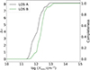 |
Fig. 1. Redshift path (Δz) and completeness for the line-of-sight A (B) in black (green) as a function of the column density threshold (Nmin). |
3. Absorption line analysis
3.1. Absorption line identification and fitting
To identify C IV absorption systems, we automatically searched for peaks in the optical depth in the wavelength range between Lyα and C IV emission lines and selected those by eye that were compatible with the doublet line separation and the doublet ratio. This approach identified 73 systems for lines-of-sight A and 68 for lines-of-sight B. To accurately measure the redshifts of the individual C IV velocity components on each absorption system, we fit Voigt profiles to each system using the Python package VoigtFit (Krogager 2018). Before the fit, we masked each region for bad pixels. When interlopers overlapped with a C IV absorption system, they were fit together. The fits were performed on each line of sight independently. In a first approach, we considered a fit successful when a VoigtFit model converged for the whole system. Moreover, we computed a component-by-component badness parameter (Churchill et al. 2020),
![Mathematical equation: $$ \begin{aligned} \text{ badness} = \Bigg {[}\Bigg {(}\dfrac{\sigma _N}{N}\Bigg {)}^2 + \Bigg {(}\dfrac{\sigma _b}{b}\Bigg {)}^2 + \Bigg {(}\dfrac{\sigma _z}{z}\Bigg {)}^2\Bigg {]}^{1/2}, \end{aligned} $$](/articles/aa/full_html/2026/03/aa58133-25/aa58133-25-eq5.gif) (3)
(3)
where σN, σb, and σz, are the uncertainties determined by VoigtFit for column density (N), Doppler parameter (b), and redshift (z), respectively. Individual velocity components with badness > 1.5 were refit with different initial parameters. This robustness check helped us to find more physically motivated components and avoided unreasonably large or small results for the fit parameters without much intervention. The final accepted fits were still a human decision, however. Considering all pairs, we found 327 C IV velocity components in lines-of-sight A and 293 in lines-of-sight B. The redshift range of this sample is 1.51 < z < 3.23. Fig. 2 shows two examples of absorption systems, along with their Voigt profile fits, at two extreme comoving transverse separations, Δr. Qualitatively, this comparison suggests that smaller Δr probes more coherent structures than larger Δr.
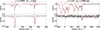 |
Fig. 2. Examples of C IV absorption systems and their Voigt profiles fits. Left panel: Absorption system at zabs = 2.2008 toward the lensed quasar HE 1104-1805. Right panel: Absorption system at zabs = 2.43 toward J234628+124858 and J234625+124743. The top (bottom) panels correspond to line-of-sight A (B). The black histogram corresponds to the normalized flux of the quasars, and the red lines correspond to the Voigt profile fit of the system. The velocity zeropoint was chosen by eye around the 1548 Å C IV line. |
3.2. Column density distribution
Another way to assess the completeness of our sample is the column density distribution, f(N, z). We calculated f(N, z) following Eqs. (6) and (7) of Zafar et al. (2013). In Fig. 3, we show f(N, z) independently for lines-of-sight A and B. This distribution can be fit by a power law, f(N, z) = C × N−δ, where C is a normalization constant, and δ is the slope of the power law. We obtained the best-fit parameters log(C) = 9.00 ± 0.78, and δ = 1.66 ± 0.06 for lines-of-sight A, and for lines-of-sight B, we found log(C) = 10.58 ± 1.81, and δ = 1.77 ± 0.13. We limited these fits to N > 1013 cm−2, where A and B have similar completeness levels. Our fits agree well with previous results by Kim et al. (2013) at 1.9 < z < 3.2 (δ = 1.85 ± 0.13) and D’Odorico et al. (2010) at 1.6 < z < 3.6 (δ = 1.71 ± 0.07), who used a similar redshift path and instrumental resolution. This agreement is a strong diagnostic for the completeness of the survey and supports our confidence in the Voigt profile fitting.
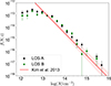 |
Fig. 3. C IV column density distribution for lines-of-sight A in black and lines-of-sight B in green. The solid pink line corresponds to the power-law fit by Kim et al. (2013) to data of 18 VLT/UVES single-quasar sightlines, and the shaded area is the 1σ uncertainty in the fit. |
3.3. Transverse line-of-sight separations
For the projected pair case, we computed Δr between lines of sight following Hogg (1999). For the lensed quasars, we calculated the separations by assuming that the lens is produced by a point-like source, following Krogager et al. (2018)
 (4)
(4)
where θ is the angular separation on the sky of the quasar images, while the angular diameter distances are DAS from the absorber to the quasar, DOL from the observer to the lens, DLS from the lens to the quasar, and DOA from the observer to the absorber. The resulting range of Δr for the sample is 20 pc ≲ Δr ≲ 2.4 Mpc. Fig. 4 shows the resulting distribution of Δr. The space between some bins is produced by gaps in the survey in which no quasar pairs were found. We chose this binning to account for roughly a similar number of velocity components in each bin without splitting the redshift path of a quasar line of sight. This binning is used throughout Section 4.
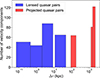 |
Fig. 4. Distribution of the C IV velocity components. The blue histogram corresponds to velocity components found on lensed quasars pairs, and the red histogram corresponds to velocity components found on projected quasar pairs. |
4. Transverse correlation analysis
4.1. Two-point correlation function
In order to study how C IV clusters at different scales, we defined the two-point correlation function, ξ(Δr, Δv), as the probability excess with respect to a randomly distributed sample,of finding a pair of velocity components with redshift zA on lines-of-sight A and zB on B with a velocity difference Δv = c|zA − zB|(1 + zAB)−1, where zAB is the average redshift, and a line-of-sight separation Δr. To compute ξ(Δr, Δv), we followed implementations similar to those by Martin et al. (2010) and Tejos et al. (2014) of the generalized Landy & Szalay (1993) estimator, in our notation:
 (5)
(5)
where DADB is the number of data-data pairs, RARB is the number of random-random pairs, and DARB and DBRA are the data-random pairs. These pairs were computed by creating every possible combination of velocity components between lines-of-sight A and B. The data-random pairs were built by pairing the data catalog from one line of sight with a random catalog generated with the other. These quantities were normalized by their respective normalization factors,
 (6)
(6)
where NA and NB are the total number of absorption lines found on lines-of-sight A and B, respectively, and α is a positive integer used to build the random catalogs, which we describe below. To create these pairs of velocity components, we only considered column densities above 90% completeness in line-of-sight B, and this same limit was applied on line-of-sight A. In total, this corresponds to 300 components in A and 249 components in B (≈88% of the total sample).
The creation of random catalogs is a delicate point when working with two-point correlation functions, as it largely depends on the geometry and type of objects involved. We followed the approach of Tejos et al. (2014) and created α = 100 copies of each measured parameter set (z, N) by randomizing their redshifts. Each random redshift was drawn uniformly from any position on the quasar line of sight where the corresponding N could have been measured, depending on the spectral coverage and the column density limit given the signal-to-noise ratio. This limiting column density was measured following Eq. (2). This way of randomizing the redshifts aids in reducing any sort of detection bias because the spectra naturally have a different signal-to-noise at different wavelengths.
The Landy & Szalay (1993) estimator is typically preferred because it minimizes the Poisson variance (ΔDD2(ξ) = (1 + ξ)/DD). When only uncertainties due to Poisson variance are assumed, however, as discussed by Mo et al. (1992) and Tejos et al. (2014), the real uncertainty might be underpredicted. To remedy this potential issue, we adopted a more conservative approach by estimating our uncertainties (ΔBS2) via bootstrapping and computed our correlation measurements NBS = 100 times with a random sample (with repetition) of NA velocity components on line-of-sight A and NB on line-of-sight B. For every bin,
 (7)
(7)
where  is the mean over all bootstrap measurements ξi. Finally, to compute ξ, each type of pairs (DADB, DARB, DBRA, RARB) was summed,
 (8)
(8)
In Fig. 5 we show 1 + ξ(Δr) binned for three values of maximum Δv as a function of Δr. The bins in separation were chosen so that each bin had roughly the same number of pairs when possible (the same binning is used in Fig. 4). The maximum Δv (200, 600, and 1000 km s−1) was chosen to compare more directly with Martin et al. (2010) (open circles), who analyzed data of 29 projected quasar pairs at a medium spectral resolution. All of these pairs are different from the 12 pairs we found on our sample, which makes our results completely independent. The figure shows that the amplitude of ξ(Δr) generally increases with decreasing separation, although at scales between ≈5 kpc and ≈500 kpc, ξ seems to be constant in three bins when it is compared with the smaller bin by Martin et al. (2010).
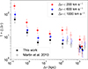 |
Fig. 5. Two-point correlation function (ξ(Δr)) of C IV as a function of the line-of-sight separation for three different velocity bins. The red and blue points are slightly shifted for clarity from their identical position to the blue points. The open circle data points correspond to the measurements obtained by Martin et al. (2010). |
4.2. Projected transverse correlations
In order to compare our measurements with galaxy autocorrelation studies and properly fit ξ(Δr), we computed the projected transverse correlation function (PTCF) (Davis & Peebles 1983). The PTCF is the integral of ξ(Δv, Δr) over the distance in redshift space (ΔΠ), which is obtained by assuming the observed Δv is produced by Hubble flow, and therefore, ΔΠ(Δv, z) = (1 + z)Δv/H(z). Then, the PTCF is computed as
 (9)
(9)
Additionally, this can be approximated because of the cylindrical symmetry of the survey following Martin et al. (2010) and Tejos et al. (2014) by
 (10)
(10)
Moreover, Davis & Peebles (1983) showed that this function can be fit using a power law with a slope γ by assuming that the correlations in real space take the form ξ(Δr) = (r0/Δr)γ. Then
 (11)
(11)
where A(r0, γ) = r0γΓ(1/2)Γ[(γ − 1)/2]/Γ(γ/2), and Γ is the gamma function. It is important to note that this assumes a γ > 1 and Πmax → ∞. Then, a fit of Ξ(Δr) intermediately provides a value for r0 and γ. In Fig. 6 we show Ξ(Δr) for the same velocity threshold bins as in Fig. 5. We chose the larger threshold because the condition for Eq. (11) is that Πmax → ∞.
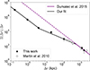 |
Fig. 6. Projected transverse correlation function (Ξ(Δr)) for C IV. The bins are the same as in Fig. 5. The open circle data points correspond to the measurements obtained by Martin et al. (2010), using the same velocity threshold and estimator. The solid purple line shows a galaxy-galaxy autocorrelation function result (Durkalec et al. 2015), with parameters |


We then fit Ξ(Δr) in three different ways. First, we fit a single power law (Eq. (11)) with best-fit parameters r0 = 4.63 ± 1.18 Mpc and γ = 1.18 ± 0.04 (see Fig. C.1). While this fit works well at higher Δr, it underpredicts the smaller separation bin, and it does not consider the relation between C IV and galaxies. With this in mind, we considered the prediction from Scannapieco et al. (2006) that ξ should break and flatten somewhere at small separations.
Following Martin et al. (2010), we modified our fit to Ξ(Δr) to add a break to the power law of the form
 (12)
(12)
where the first regime delimited by r1 is seen as a constant correlation ξ(Δr) (which when normalized is seen as Ξ(Δr)/Δr ∝ 1/Δr). Following Martin et al. (2010), we adopted the r0 and γ parameters form the galaxy autocorrelation function; this can be assumed when we consider that the correlation amplitudes of C IV and those of the galaxies are the same at scales larger than the sizes of C IV enriched regions. We chose the result of Durkalec et al. (2015) with parameters  Mpc and
  because they studied a sizable sample of 1556 galaxies in a similar redshift range 2.0 < z < 2.9. In this way, the only free parameter for this model is r1, for which we found a best fit at r1 = 597 ± 130 kpc when we considered the points from Martin et al. (2010) (see Fig. C.2). The flat ξ(Δr) prediction still shows an even larger offset at small Δr when compared with the single-power law model, however. This is also noticeable in the increasing correlations at very small scales (Δr < 10 kpc) and is best seen in Fig. 5.
Taking this into consideration, we modified Eq. (12) to add a second break on ξ(Δr) to account for a third regime at the smallest separations,
 (13)
(13)
where r2 and γ1 are the new free parameters because r3 can be determined by imposing the continuity of ξ(Δr). In this way, r3 = r2(r0/r1)γ/γ1. In Fig. 6 we present the resulting best fit for this model as the black line, corresponding to the best fit parameters:  kpc,
kpc,  kpc, and γ1 = 1.78 ± 0.10. We again used the galaxy-galaxy autocorrelation measurements of γ and r0 (Durkalec et al. 2015), and we considered the data points from Martin et al. (2010). When we follow the same reasoning from the arguments for the first break of ξ(Δr), a second break implies that these smaller scales probe a different structure than the one we see at larger separations. This model indeed fits the data much closer than the simpler models that struggle at the smaller scales, which strongly supports the idea that we probe a different type of environment at the smaller scales probed by this survey (≲10 kpc).
5. Discussion
The connection between galaxies and C IV is well documented (e.g., Adelberger et al. 2005; Martin et al. 2010; Turner et al. 2014; Bird et al. 2016; Rudie et al. 2019; Galbiati et al. 2023; Banerjee et al. 2023). For this reason, our fits from Eqs. (12) and (13) directly take the same correlation length from galaxies into account. Our correlation measurements at the higher separation bins lie exactly on top of the galaxy autocorrelations (Fig. 6) that were also found by Martin et al. (2010) when comparing with Adelberger et al. (2005). This then suggests that C IV might be a good tracer of the way in which galaxies cluster at cosmic noon. We observe, however, that the strong relation with galaxies does not hold at Δr ≲ 500 kpc, as seen in the flattening in of ξ(Δr) in Fig. 5 (this is the scale of the intermediate regime in Fig. 6, where Ξ(Δr)/Δr ∝ 1/Δr). It has been argued (Scannapieco et al. 2006; Martin et al. 2010; Mintz et al. 2022) that this flattening of ξ provides constraints on the sizes of C IV enriched regions around galaxies. The argument is based on the fact that by decreasing Δr, we do not find a significant number of additional pairs of velocity components, which then implies that we probe distances smaller than these regions. In conclusion, the break that we find on large scales with the two models from Eqs. (12) and (13) (597 ± 130 kpc and  kpc) agrees well with the result reported by Martin et al. (2010) of r1 = 600 ± 214 kpc.
On the other hand, at the smaller scales probed here, Fig. 5 shows that ξ(Δr) increases again. We attribute this to the fact that at this scale, the autocorrelation is dominated by pairs of velocity components on the same absorption system. Therefore, this second break at  kpc would provide limits on the sizes of individual C IV clouds within the CGM of galaxies, instead of whole absorption systems. Unfortunately, the sizes of these clouds are difficult to constrain. For instance, Rauch et al. (2001) measured characteristic sizes of C IV clouds in the range r0 = [3, 19] kpc, also using lensed quasars, but a different method to constrain sizes. On the other hand, Lopez et al. (2024) found rather smaller sizes (≲1 kpc) from kinematic arguments, but concentrated on the very strong C IV systems toward gravitational arcs. The existence of a break in ξ at
  kpc, as shown in this work, strongly supports the idea of a coherence length of the cool-warm CGM at the scale of a few kiloparsec.
It is worth comparing our results with those for other species. Also using gravitational arcs, Afruni et al. (2023) measured a coherence length of 4.2−2.8+3.6 kpc by studying absorption systems of Mg II at lower redshifts (z ≈ 1). Interestingly, this result is well within 1σ from ours, even when we consider that C IV is more ionized and typically covers a larger cross section than Mg II (e.g., Dutta et al. 2021). Independently, Rubin et al. (2018) measured a lower length for the coherence length of 1.9 kpc, which is still consistent with our result, but might also indicate a possible difference between the coherence length of these ions. Therefore, further work is needed to assess a possible difference between these coherence scales.
It is also interesting to make a comparison with independent measurements of the clustering of C IV systems. To do this, we first projected ξ(Δv, Δr) in velocity. Fig. 7 shows ξ(Δv) in two bins around Δr = 10 kpc. Notably, the amplitudes of ξ(Δv) in the two bins are quite different, which is expected given the results of Section 4. This difference makes a direct comparison with single quasar line of sight results more difficult, however. At small separations, ξ(Δv) becomes comparable with the velocity clustering measured directly toward single quasar lines of sight (green points), obtained using data with a similar resolution at z ≈ 2.2 (Scannapieco et al. 2006). Based on this similarity, we fit our ξ(Δv) points at Δr < 10 kpc using two Gaussians following Boksenberg & Sargent (2015),
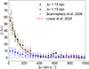 |
Fig. 7. Two-point correlation function (ξ(Δv)) of C IV as a function of velocity across the two lines of sight for two different bins in separation, shown as the black and blue points for Δr < 10 kpc and Δr > 10 kpc, respectively. The green points correspond to the single line-of-sight measurements obtained by Scannapieco et al. (2006). The dashed red line shows a prediction from transverse correlations of C IV using gravitational arcs (Lopez et al. 2024), adjusted to account for the different spectral and spatial resolution. |
 (14)
(14)
where A1, 2 are the amplitudes, and σ1, 2 the corresponding standard deviations. We obtained a best fit with A1 = 26.2 ± 15.3, σ1 = 48.8 ± 33 km s−1, A2 = 29.5 ± 11.7, and σ2 = 166.3 ± 28.4 km s−1. These standard deviations are consistent with those obtained by Boksenberg & Sargent (2015) at σ1, 2 = 35.5, 105 km s−1, suggesting that ξ(Δv) as measured by quasar pairs at small separations, where absorption profiles become more similar, is comparable to that measured using single lines of sight.
In an independent comparison, the dashed red line of Fig. 7 shows the measurement obtained by Lopez et al. (2024). These authors computed a transverse ξ(Δv) for C IV absorption systems using a different technique, namely integral field spectroscopy of giant gravitational arcs, over separations of Δr ≲ 10 kpc. When we use the relation between σ of ξ for arcs and QSOs proposed by these authors, namely,  , where N is the mean number of clouds per spatial resolution element in Lopez et al. (2024), we obtain the relation shown by the dashed red line. This relation matches our measurements at Δr < 10 kpc remarkably well considering the different methods. We conclude that measurements of ξ toward point-like and extended sources are indeed consistent with each other.
6. Summary
We assembled a sample of high-resolution spectra of 12 quasar pairs to study the clustering of C IV absorption systems around cosmic noon. Our results are listed below.
-
We detected 141 C IV absorption systems at z ≈ 2, in parallel quasar line of sights (A and B) spanning separations between 20 pc and up to 2.37 Mpc.
-
We fit Voigt profiles to all velocity components, which resulted in a sample of 327 C IV velocity components on lines-of-sight A and 293 on lines-of-sight B, with a column density distribution that agreed with the known C IV statistics (Fig. 3).
-
We computed the two-point correlation function of C IV velocity components (ξ(Δv, Δr)) using the Landy & Szalay (1993) estimator (Fig. 5). We found that the amplitude of ξ(Δr) flattens in the ≈10 − 500 kpc range, which confirms previous predictions of flattening for the ξ(Δr) in this range (Martin et al. 2010; Mintz et al. 2022).
-
We computed the projected transverse correlation function (Ξ(Δr)) (Fig. 6). We then tested models of broken power laws to estimate the coherence length of C IV absorption systems. For the larger scales we found a best fit at
 kpc, which we consider the scale of these metal-enriched regions.
 -
For the smaller scales (≲10 kpc), the correlation amplitude increases with decreasing separation. This suggests a different regime of the correlation function at scales
 kpc, which we interpret as a relevant scale for the coherence length of C IV clouds.
 -
Our results offer the first comprehensive picture of the clustering of metal-enriched regions and shows that they are separately compatible with observations of C IV toward giant gravitational arcs (Fig. 7), previous measurements of cloud sizes for C IV, and the coherence length of the CGM.
While our results suggest a small coherence length of C IV clouds, further work is necessary to measure more precise correlation amplitudes at separations ≲1 kpc. To achieve this, more spectroscopic data on lensed quasars (or galaxies) are needed. On larger scales, additional data on quasars pairs would significantly help us to constrain the scale of the metal-enriched regions, whose uncertainties are still on the order of hundreds of kiloparsecs.
Acknowledgments
We would like to thank the anonymous referee for their constructive feedback and comments. H. C., S. L. and N. T. acknowledge the support by FONDECYT grant 1231187. P. A. acknowledges support from ANID-Subdirección de Capital Humano/Doctorado Nacional/2022-21222110.
References
- Adelberger, K. L., Shapley, A. E., Steidel, C. C., et al. 2005, ApJ, 629, 636 [NASA ADS] [CrossRef] [Google Scholar]
- Afruni, A., Lopez, S., Anshul, P., et al. 2023, A&A, 680, A112 [NASA ADS] [CrossRef] [EDP Sciences] [Google Scholar]
- Banerjee, E., Muzahid, S., Schaye, J., Johnson, S. D., & Cantalupo, S. 2023, MNRAS, 524, 5148 [NASA ADS] [CrossRef] [Google Scholar]
- Bird, S., Rubin, K. H. R., Suresh, J., & Hernquist, L. 2016, MNRAS, 462, 307 [NASA ADS] [CrossRef] [Google Scholar]
- Boksenberg, A., & Sargent, W. L. W. 2015, ApJS, 218, 7 [NASA ADS] [CrossRef] [Google Scholar]
- Bolmer, J., Greiner, J., Krühler, T., et al. 2018, A&A, 609, A62 [NASA ADS] [CrossRef] [EDP Sciences] [Google Scholar]
- Bordoloi, R., Wagner, A. Y., Heckman, T. M., & Norman, C. A. 2017, ApJ, 848, 122 [Google Scholar]
- Bordoloi, R., O’Meara, J. M., Sharon, K., et al. 2022, Nature, 606, 59 [NASA ADS] [CrossRef] [Google Scholar]
- Chen, H.-W., Gauthier, J.-R., Sharon, K., et al. 2014, MNRAS, 438, 1435 [NASA ADS] [CrossRef] [Google Scholar]
- Chen, Y., Steidel, C. C., Hummels, C. B., et al. 2020, MNRAS, 499, 1721 [NASA ADS] [CrossRef] [Google Scholar]
- Churchill, C. W., Evans, J. L., Stemock, B., et al. 2020, ApJ, 904, 28 [Google Scholar]
- Cooke, J., & O’Meara, J. M. 2015, ApJ, 812, L27 [NASA ADS] [CrossRef] [Google Scholar]
- Cooksey, K. L., Kao, M. M., Simcoe, R. A., O’Meara, J. M., & Prochaska, J. X. 2013, ApJ, 763, 37 [NASA ADS] [CrossRef] [Google Scholar]
- Coppolani, F., Petitjean, P., Stoehr, F., et al. 2006, MNRAS, 370, 1804 [NASA ADS] [CrossRef] [Google Scholar]
- Cristiani, S., Cupani, G., Trost, A., et al. 2024, MNRAS, 528, 6845 [Google Scholar]
- Davis, M., & Peebles, P. J. E. 1983, ApJ, 267, 465 [Google Scholar]
- Dekker, H., D’Odorico, S., Kaufer, A., Delabre, B., & Kotzlowski, H. 2000, SPIE Conf. Ser., 4008, 534 [Google Scholar]
- D’Odorico, V., Viel, M., Saitta, F., et al. 2006, MNRAS, 372, 1333 [Google Scholar]
- D’Odorico, V., Calura, F., Cristiani, S., & Viel, M. 2010, MNRAS, 401, 2715 [Google Scholar]
- D’Odorico, V., Cupani, G., Cristiani, S., et al. 2013, MNRAS, 435, 1198 [CrossRef] [Google Scholar]
- Durkalec, A., Le Fèvre, O., Pollo, A., et al. 2015, A&A, 583, A128 [NASA ADS] [CrossRef] [EDP Sciences] [Google Scholar]
- Dutta, R., Fumagalli, M., Fossati, M., et al. 2021, MNRAS, 508, 4573 [NASA ADS] [CrossRef] [Google Scholar]
- Dutta, R., Acebron, A., Fumagalli, M., et al. 2024, MNRAS, 528, 1895 [CrossRef] [Google Scholar]
- Faucher-Giguère, C.-A., & Kereš, D. 2011, MNRAS, 412, L118 [CrossRef] [Google Scholar]
- Faucher-Giguère, C.-A., & Oh, S. P. 2023, ARA&A, 61, 131 [CrossRef] [Google Scholar]
- Fernandez-Figueroa, A., Lopez, S., Tejos, N., et al. 2022, MNRAS, 517, 2214 [NASA ADS] [CrossRef] [Google Scholar]
- Galbiati, M., Fumagalli, M., Fossati, M., et al. 2023, MNRAS, 524, 3474 [NASA ADS] [CrossRef] [Google Scholar]
- Hasan, F., Churchill, C. W., Stemock, B., et al. 2020, ApJ, 904, 44 [Google Scholar]
- Hennawi, J. F., Strauss, M. A., Oguri, M., et al. 2006, AJ, 131, 1 [Google Scholar]
- Hogg, D. W. 1999, ArXiv e-prints [arXiv:astro-ph/9905116] [Google Scholar]
- Kereš, D., Katz, N., Weinberg, D. H., & Davé, R. 2005, MNRAS, 363, 2 [Google Scholar]
- Kim, T. S., Partl, A. M., Carswell, R. F., & Müller, V. 2013, A&A, 552, A77 [NASA ADS] [CrossRef] [EDP Sciences] [Google Scholar]
- Krogager, J.-K. 2018, ArXiv e-prints [arXiv:1803.01187] [Google Scholar]
- Krogager, J. K., Noterdaeme, P., O’Meara, J. M., et al. 2018, A&A, 619, A142 [NASA ADS] [CrossRef] [EDP Sciences] [Google Scholar]
- Krogager, J. K., De Cia, A., Heintz, K. E., et al. 2024, MNRAS, 535, 561 [Google Scholar]
- Landy, S. D., & Szalay, A. S. 1993, ApJ, 412, 64 [Google Scholar]
- Lehner, N., Wotta, C. B., Howk, J. C., et al. 2018, ApJ, 866, 33 [Google Scholar]
- Lopez, S., Reimers, D., Rauch, M., Sargent, W. L. W., & Smette, A. 1999, ApJ, 513, 598 [NASA ADS] [CrossRef] [Google Scholar]
- Lopez, S., Reimers, D., Gregg, M. D., et al. 2005, ApJ, 626, 767 [NASA ADS] [CrossRef] [Google Scholar]
- Lopez, S., Ellison, S., D’Odorico, S., & Kim, T. S. 2007, A&A, 469, 61 [NASA ADS] [CrossRef] [EDP Sciences] [Google Scholar]
- Lopez, S., Tejos, N., Ledoux, C., et al. 2018, Nature, 554, 493 [NASA ADS] [CrossRef] [Google Scholar]
- Lopez, S., Tejos, N., Barrientos, L. F., et al. 2020, MNRAS, 491, 4442 [NASA ADS] [CrossRef] [Google Scholar]
- Lopez, S., Afruni, A., Zamora, D., et al. 2024, A&A, 691, A356 [NASA ADS] [CrossRef] [EDP Sciences] [Google Scholar]
- Maitra, S., Srianand, R., Petitjean, P., et al. 2019, MNRAS, 490, 3633 [NASA ADS] [CrossRef] [Google Scholar]
- Martin, C. L., Scannapieco, E., Ellison, S. L., et al. 2010, ApJ, 721, 174 [NASA ADS] [CrossRef] [Google Scholar]
- Mintz, A., Rafelski, M., Jorgenson, R. A., et al. 2022, AJ, 164, 51 [NASA ADS] [CrossRef] [Google Scholar]
- Mo, H. J., Jing, Y. P., & Boerner, G. 1992, ApJ, 392, 452 [NASA ADS] [CrossRef] [Google Scholar]
- Mortensen, K., Keerthi Vasan, G. C., Jones, T., et al. 2021, ApJ, 914, 92 [CrossRef] [Google Scholar]
- Murphy, M. T., Kacprzak, G. G., Savorgnan, G. A. D., & Carswell, R. F. 2019, MNRAS, 482, 3458 [NASA ADS] [CrossRef] [Google Scholar]
- Nelson, D., Genel, S., Pillepich, A., et al. 2016, MNRAS, 460, 2881 [NASA ADS] [CrossRef] [Google Scholar]
- O’Meara, J. M., Lehner, N., Howk, J. C., et al. 2015, AJ, 150, 111 [Google Scholar]
- O’Meara, J. M., Lehner, N., Howk, J. C., et al. 2017, AJ, 154, 114 [CrossRef] [Google Scholar]
- Oppenheimer, B. D., & Davé, R. 2006, MNRAS, 373, 1265 [NASA ADS] [CrossRef] [Google Scholar]
- Péroux, C., & Howk, J. C. 2020, ARA&A, 58, 363 [CrossRef] [Google Scholar]
- Prochaska, J. X., Tejos, N., Crighton, N., et al. 2016, https://doi.org/10.5281/zenodo.168270 [Google Scholar]
- Prochter, G. E., Prochaska, J. X., & Burles, S. M. 2006, ApJ, 639, 766 [NASA ADS] [CrossRef] [Google Scholar]
- Rauch, M., Sargent, W. L. W., & Barlow, T. A. 1999, ApJ, 515, 500 [NASA ADS] [CrossRef] [Google Scholar]
- Rauch, M., Sargent, W. L. W., & Barlow, T. A. 2001, ApJ, 554, 823 [NASA ADS] [CrossRef] [Google Scholar]
- Rubin, K. H. R., Prochaska, J. X., Koo, D. C., et al. 2014, ApJ, 794, 156 [Google Scholar]
- Rubin, K. H. R., Diamond-Stanic, A. M., Coil, A. L., Crighton, N. H. M., & Stewart, K. R. 2018, ApJ, 868, 142 [NASA ADS] [CrossRef] [Google Scholar]
- Rudie, G. C., Steidel, C. C., Pettini, M., et al. 2019, ApJ, 885, 61 [NASA ADS] [CrossRef] [Google Scholar]
- Saccardi, A., Vergani, S. D., De Cia, A., et al. 2023, A&A, 671, A84 [NASA ADS] [CrossRef] [EDP Sciences] [Google Scholar]
- Savage, B. D., & Sembach, K. R. 1991, ApJ, 379, 245 [NASA ADS] [CrossRef] [Google Scholar]
- Scannapieco, E., Pichon, C., Aracil, B., et al. 2006, MNRAS, 365, 615 [NASA ADS] [CrossRef] [Google Scholar]
- Schaye, J., Aguirre, A., Kim, T.-S., et al. 2003, ApJ, 596, 768 [Google Scholar]
- Songaila, A. 2005, AJ, 130, 1996 [NASA ADS] [CrossRef] [Google Scholar]
- Steidel, C. C., Erb, D. K., Shapley, A. E., et al. 2010, ApJ, 717, 289 [Google Scholar]
- Taylor, M. B. 2020, ASP Conf. Ser., 522, 67 [Google Scholar]
- Tejos, N., Lopez, S., Prochaska, J. X., Chen, H.-W., & Dessauges-Zavadsky, M. 2007, ApJ, 671, 622 [Google Scholar]
- Tejos, N., Lopez, S., Prochaska, J. X., et al. 2009, ApJ, 706, 1309 [Google Scholar]
- Tejos, N., Morris, S. L., Finn, C. W., et al. 2014, MNRAS, 437, 2017 [Google Scholar]
- Tejos, N., López, S., Ledoux, C., et al. 2021, MNRAS, 507, 663 [NASA ADS] [CrossRef] [Google Scholar]
- Tumlinson, J., Peeples, M. S., & Werk, J. K. 2017, ARA&A, 55, 389 [Google Scholar]
- Turner, M. L., Schaye, J., Steidel, C. C., Rudie, G. C., & Strom, A. L. 2014, MNRAS, 445, 794 [NASA ADS] [CrossRef] [Google Scholar]
- Urbano Stawinski, S. M., Rubin, K. H. R., Prochaska, J. X., et al. 2023, ApJ, 951, 135 [NASA ADS] [CrossRef] [Google Scholar]
- Vergani, S. D., Petitjean, P., Ledoux, C., et al. 2009, A&A, 503, 771 [NASA ADS] [CrossRef] [EDP Sciences] [Google Scholar]
- Vogt, S. S., Allen, S. L., Bigelow, B. C., et al. 1994, SPIE Conf. Ser., 2198, 362 [NASA ADS] [Google Scholar]
- Welsh, L., D’Odorico, V., Fontanot, F., et al. 2025, A&A, 703, A274 [NASA ADS] [CrossRef] [EDP Sciences] [Google Scholar]
- Zafar, T., Péroux, C., Popping, A., et al. 2013, A&A, 556, A141 [NASA ADS] [CrossRef] [EDP Sciences] [Google Scholar]
- Zahedy, F. S., Chen, H.-W., Rauch, M., Wilson, M. L., & Zabludoff, A. 2016, MNRAS, 458, 2423 [NASA ADS] [CrossRef] [Google Scholar]
Appendix A: Integral Constraint
A well known bias in correlation measurements that we did not address in the main text is the so-called "integral constraint". This comes from the fact that the redshift space of each quasar is limited. Then, when we measure positive correlation, this can cause a negative one somewhere else, but at the same time the real correlation can be assumed to be positive. As shown by Landy & Szalay (1993), the real correlation (ξreal) is related to the measured one (ξ) by:
 (A.1)
(A.1)
where ξV is the integral constraint computed as follows:
 (A.2)
(A.2)
with G(r) = RARB/nRR. As we do not know ξreal a priori, we only made a small correction following Tejos et al. (2014),
 (A.3)
(A.3)
which is a small correction in this case (≲1%), smaller than our uncertainties. We nonetheless applied this correction.
Appendix B: Continuity of the projected transverse correlation function.
Imposing the continuity of Ξ, at Δr = r2, it is immediate that,
 (B.1)
(B.1)
Appendix C: Additional fits to the projected transverse correlation function.
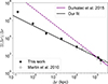 |
Fig. C.1. Projected transverse correlation function (Ξ(Δr)) for C IV. Same as Fig. 6, with the difference that here we fit a single power law of the form shown in Eq. 11. Best fit parameters: r0 = 4.45 ± 0.56 Mpc, and γ = 1.17 ± 0.05. |
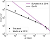 |
Fig. C.2. Projected transverse correlation function (Ξ(Δr)) for C IV. Same as Fig. 6, with the difference that here we fit a broken power law of the form shown in Eq. 12. Best fit parameter: r1 = 597 ± 130. |
All Tables
All Figures
|
Fig. 1. Redshift path (Δz) and completeness for the line-of-sight A (B) in black (green) as a function of the column density threshold (Nmin). |
| In the text | |
|
Fig. 2. Examples of C IV absorption systems and their Voigt profiles fits. Left panel: Absorption system at zabs = 2.2008 toward the lensed quasar HE 1104-1805. Right panel: Absorption system at zabs = 2.43 toward J234628+124858 and J234625+124743. The top (bottom) panels correspond to line-of-sight A (B). The black histogram corresponds to the normalized flux of the quasars, and the red lines correspond to the Voigt profile fit of the system. The velocity zeropoint was chosen by eye around the 1548 Å C IV line. |
| In the text | |
|
Fig. 3. C IV column density distribution for lines-of-sight A in black and lines-of-sight B in green. The solid pink line corresponds to the power-law fit by Kim et al. (2013) to data of 18 VLT/UVES single-quasar sightlines, and the shaded area is the 1σ uncertainty in the fit. |
| In the text | |
|
Fig. 4. Distribution of the C IV velocity components. The blue histogram corresponds to velocity components found on lensed quasars pairs, and the red histogram corresponds to velocity components found on projected quasar pairs. |
| In the text | |
|
Fig. 5. Two-point correlation function (ξ(Δr)) of C IV as a function of the line-of-sight separation for three different velocity bins. The red and blue points are slightly shifted for clarity from their identical position to the blue points. The open circle data points correspond to the measurements obtained by Martin et al. (2010). |
| In the text | |
|
Fig. 6. Projected transverse correlation function (Ξ(Δr)) for C IV. The bins are the same as in Fig. 5. The open circle data points correspond to the measurements obtained by Martin et al. (2010), using the same velocity threshold and estimator. The solid purple line shows a galaxy-galaxy autocorrelation function result (Durkalec et al. 2015), with parameters |
| In the text | |
|
Fig. 7. Two-point correlation function (ξ(Δv)) of C IV as a function of velocity across the two lines of sight for two different bins in separation, shown as the black and blue points for Δr < 10 kpc and Δr > 10 kpc, respectively. The green points correspond to the single line-of-sight measurements obtained by Scannapieco et al. (2006). The dashed red line shows a prediction from transverse correlations of C IV using gravitational arcs (Lopez et al. 2024), adjusted to account for the different spectral and spatial resolution. |
| In the text | |
|
Fig. C.1. Projected transverse correlation function (Ξ(Δr)) for C IV. Same as Fig. 6, with the difference that here we fit a single power law of the form shown in Eq. 11. Best fit parameters: r0 = 4.45 ± 0.56 Mpc, and γ = 1.17 ± 0.05. |
| In the text | |
|
Fig. C.2. Projected transverse correlation function (Ξ(Δr)) for C IV. Same as Fig. 6, with the difference that here we fit a broken power law of the form shown in Eq. 12. Best fit parameter: r1 = 597 ± 130. |
| In the text | |
Current usage metrics show cumulative count of Article Views (full-text article views including HTML views, PDF and ePub downloads, according to the available data) and Abstracts Views on Vision4Press platform.
Data correspond to usage on the plateform after 2015. The current usage metrics is available 48-96 hours after online publication and is updated daily on week days.
Initial download of the metrics may take a while.