| Issue |
A&A
Volume 707, March 2026
|
|
|---|---|---|
| Article Number | A202 | |
| Number of page(s) | 12 | |
| Section | Galactic structure, stellar clusters and populations | |
| DOI | https://doi.org/10.1051/0004-6361/202558155 | |
| Published online | 13 March 2026 | |
The LEGARE Project
I. Chemical evolution model of the Nuclear Stellar Disc in a Bayesian framework
1
I.N.A.F. Osservatorio Astronomico di Trieste,
via G.B. Tiepolo 11,
34143
Trieste,
Italy
2
IFPU, Institute for Fundamental Physics of the Universe,
Via Beirut 2,
34151
Trieste,
Italy
3
Université Côte d’Azur, Observatoire de la Côte d’Azur, Laboratoire Lagrange, CNRS, Blvd de l’Observatoire,
06304
Nice,
France
4
Dipartimento di Fisica, Sezione di Astronomia, Università di Trieste,
Via G. B. Tiepolo 11,
34143
Trieste,
Italy
5
INFN Sezione di Trieste,
via Valerio 2,
34134
Trieste,
Italy
6
Division of Astrophysics, Department of Physics, Lund University,
Box 118,
221 00
Lund,
Sweden
7
ICSC – Italian Research Center on High Performance Computing, Big Data and Quantum Computing,
Via Magnanelli 2,
40033
Casalecchio di Reno,
Italy
8
Como Lake centre for AstroPhysics (CLAP), DiSAT, Università dell’Insubria,
via Valleggio 11,
Como
22100,
Italy
★ Corresponding author: This email address is being protected from spambots. You need JavaScript enabled to view it.
Received:
17
November
2025
Accepted:
28
January
2026
Abstract
Context. The nuclear stellar disc (NSD) of the Milky Way is a dense, rotating stellar system in the central ~200 pc. The NSD is thought to be primarily fuelled by bar-driven gas inflows from the inner Galactic disc.
Aims. As part of the LEGARE project, we aim to construct the first chemical-evolution models for the NSD using a Bayesian approach tailored to reproducing the observed metallicity-distribution functions and compared with the available abundance ratios for Mg, Si, and Ca relative to Fe. In particular, we intend to test whether the flowing gas from the inner Galactic disc, which feeds the NSD, can reproduce the observed abundances.
Methods. We adopted a state-of-the-art chemical-evolution model in which the gas responsible for the formation of the NSD is assumed to be driven by the Galactic-bar-induced inflows. The chemical composition of the accreted material is assumed to reflect that of the Galactic disc at a radius of ~4 kpc. A Bayesian framework based on Markov Chain Monte Carlo (MCMC) techniques was then employed to fit the metallicity-distribution functions of different samples of NSD stars.
Results. If we take the NSD data at face value, without considering possible contamination from bulge stars, we find that a formation scenario based on the inner disc’s flowing gas is inconsistent with the low-metallicity tail of the observed metallicity-distribution function. This is because the inner disc’s metallicity, at the epoch of bar formation, was already near solar. On the other hand, models invoking dilution from additional metal-poor inflows successfully reproduce the observations. Models with different levels of gas dilution share similar gas infall timescales (ranging from 3.7 to 5.2 Gyr) and negligible galactic winds (mass-loading factors, ω, between 0.001 and 0.030). The best-fit model corresponds to an inflow with a metallicity five times lower than that of the inner disc and a moderate star-formation efficiency. The same model successfully reproduces the observed [α/Fe] − [Fe/H] abundance trends and predicts a star formation history consistent with the most recent estimates. However, if we assume that the metallicity distribution function is contaminated by metal-poor bulge stars and is restricted to stars with [Fe/H] > −0.3 dex, there is no longer any need for gas dilution. In this case, the best-fit model is characterised by a very low star formation efficiency, coupled with a mild galactic wind.
Conclusions. Our analysis indicates that dilution of the inflowing gas forming the NSD is necessary to reproduce its observed chemical properties, if bulge contamination in the data is not considered. This implies that, in addition to bar-driven inflows from the inner thin disc, lower metallicity gas – possibly originating from the thick disc or from more recent accretion events – contributed to the formation of the NSD. On the other hand, when contamination by bulge stars is assumed, dilution is no longer required.
Key words: ISM: abundances / Galaxy: abundances / Galaxy: disk / Galaxy: evolution / Galaxy: formation
© The Authors 2026
 Open Access article, published by EDP Sciences, under the terms of the Creative Commons Attribution License (https://creativecommons.org/licenses/by/4.0), which permits unrestricted use, distribution, and reproduction in any medium, provided the original work is properly cited.
This article is published in open access under the Subscribe to Open model. This email address is being protected from spambots. You need JavaScript enabled to view it. to support open access publication.
1 Introduction
The central regions of the Milky Way provide a unique laboratory in which to study the interplay between gas dynamics, star formation, and chemical enrichment. The nuclear stellar disc (NSD) is a significant component within the central region of our Milky Way, alongside the nuclear star cluster (NSC) and the central massive black hole (see Schultheis et al. 2025 for a review and references therein). Among these structures, the NSD stands out as a massive, rotating component confined within the central few hundred parsecs, with a scale radius of ~100 pc and a scale height of around 50 pc; these are characterised by a stellar mass of the order of 109 M⊙ (Launhardt et al. 2002; Nogueras-Lara et al. 2020). Its high stellar density, rapid rotation, and distinct geometry relative to the surrounding bulge make the NSD a key tracer of the secular evolution of the Galaxy.
The stellar composition of the NSD has been relatively unexplored until recent times, primarily due to challenges such as extreme extinction and stellar crowding. NSDs are also seen in extragalactic systems and show an inside-out formation (e.g. Bittner et al. 2020). The Galactic bar is a structure that cannot be ignored if we want to properly describe the evolution of the NSD. Simulations suggest that most of the NSD mass forms within ~1 Gyr of the bar formation (Baba & Kawata 2020; Cole et al. 2014). Hence, the NSD star formation history can be used to estimate the age of the Galactic bar. Similarly to most disc galaxies, the Milky Way features a central Galactic bar that dominates approximately the inner 4 kpc. As the bar sweeps through the gas in the Galactic disc, it creates long shock lanes along its leading edges and tips (Athanassoula 1992). This gas falls on the leading side of the bar into the central region and accumulates on the dense nuclear disc (Contopoulos & Grosbol 1989). The recent work of Nieuwmunster et al. (2024) presented a detailed orbital analysis of stars located in the NSD of the Milky Way and investigated the dynamical history of this structure. Based on a detailed orbital analysis, the authors were able to classify orbits into various families, most of which are characterised by x2-type orbits, which are dominant in the inner part of the bar. This is another confirmation that the NSD evolution is strictly linked with the destiny of the Galactic bar.
Recent observational progress has brought the NSD into sharper focus. Using VLT-KMOS, Schultheis et al. (2021) demonstrated that the NSD is chemically and kinematically distinct from both the Galactic bulge and the NSC. Metal-rich stars display a dynamically cool component with lower velocity dispersion, likely formed from gas in the central molecular zone (CMZ), while the origin of the more metal-poor population remains debated. The GALACTICNUCLEUS survey has also provided exquisite photometric constraints, revealing a complex star formation history with evidence of both old and intermediate-age populations (Nogueras-Lara et al. 2021). At the chemical level, recent high-resolution abundance studies have delivered unprecedented detail. Ryde et al. (2025) used IGRINS/Gemini South to measure abundances of 18 elements in nine NSD M giants, covering −1.0 ≲ [Fe/H] ≲ +0.5. Their results show strong similarities with inner-disc and innerbulge populations at sub-solar metallicity, while at super-solar metallicity the NSD follows the trends of the NSC. These results demonstrate that high-quality chemical abundances can be obtained even in the heavily extincted Galactic centre, opening the way for large-scale spectroscopic programs such as the Multi-Object Optical and Near-infrared Spectrograph (MOONS, Cirasuolo et al. 2020).
Despite this progress, dedicated chemical evolution models of the NSD remain scarce. While many studies have successfully modelled the bulge in different regions (e.g. Matteucci et al. 2019; Nieuwmunster et al. 2023) and the Galactic centre (Grieco et al. 2015; Thorsbro et al. 2020), the NSD’s unique environment – shaped by bar-driven gas inflows, CMZ dynamics, and intense star formation – requires a tailored approach. In particular, Friske & Schönrich (2025) recently attempted to model the chemo-dynamical evolution of the NSD. While their models provide valuable insights into the role of gas inflows and dynamical processes, their predicted abundance ratio in the gas-phase trends display significantly more irregular behaviour than what Ryde et al. (2025) showed; that is, smooth [α/Fe] versus [Fe/H] sequences at more extended metallicities. Moreover, no comparison has been made with the available metallicity distributions of NSD stars.
As part of the Linking the chemical Evolution of Galactic discs AcRoss diversE scales (LEGARE) project, we present a new chemical-evolution model for the NSD, which we developed within a Bayesian framework. Our approach aims to directly reproduce the metallicity-distribution function (MDF) of a sub-sample from the Schultheis et al. (2021) analysis. This allowed us to quantitatively test different scenarios for the chemical composition of the gas flows responsible for the NSD’s formation and to derive robust posterior distributions for the model’s key parameters. We assumed that the inflowing gas’s composition is driven by bar-induced inflows from the inner galactic disc, consistently with the formation of the Galactic bar approximately 8 Gyr ago, as described by Sanders et al. (2024). This approach enabled us to robustly quantify parameter degeneracies and uncertainties within our NSD model; it is thus a crucial step for building a reliable and data-driven analysis. The adopted methodology closely follows the framework introduced by Spitoni et al. (2020, 2021), which included MCMC techniques to explore the parameter space of Galactic-disc chemical-evolution models.
Our paper is organised as follows. In Section 2, we present the chemical-evolution models for the inner Galactic disc and the NSD. In Section 3, the data sample used in the MCMC analysis is described. The fitting procedure is outlined in Section 4. Finally, our model results and conclusions are presented in Sections 5 and 6, respectively.
2 Chemical-evolution models
In this section, we present the chemical-evolution models adopted in this study. Section 2.1 describes the chemical evolution of the inner Galactic disc at a radius of 4 kpc, following the framework of Spitoni et al. (2021), while Section 2.2 introduces the details of the new model developed for the NSD.
2.1 Chemical-evolution model for the inner Galactic disc
In Spitoni et al. (2021), the authors presented a multi-zone, two-infall chemical-evolution model designed to reproduce APOGEE DR16 (Ahumada et al. 2020) abundance ratios at different galactocentric distances using a Bayesian analysis based on MCMC methods. For this work, we considered the best model for the innermost Galactic region’s disc computed at 4 kpc.
To trace the evolution of the thick- and thin-disc components, they adopted a two-infall prescription for the gas accretion, of which the functional form for the infall rate at 4 kpc is
![Mathematical equation: $\[\mathcal{I}_{4 D, i}(t)=X_{1, i}\left(A e^{-t / \mathrm{T}_{\text {high }}}\right)+X_{2, i}\left(\theta\left(t-\mathrm{T}_{\mathrm{d}}\right) B e^{-\left(t-\mathrm{T}_{\mathrm{d}}\right) / \mathrm{T}_{\text {low }}}\right),\]$](/articles/aa/full_html/2026/03/aa58155-25/aa58155-25-eq1.png) (1)
(1)
where Thigh=0.11 Gyr and Tlow=0.376 Gyr, are the timescales of the two distinct gas-infall episodes. The Heaviside step function is represented by θ. X1,i and X2,i represent the abundance by mass units of the element i in the two different infalling gasses. Spitoni et al. (2021) suggested that the infall has a primordial composition for the high-α, whereas for the second gas infall a chemical enrichment must be obtained from the model of the high-α disc phase corresponding to [Fe/H]=−0.5 dex. Finally, the coefficients A and B are associated with the surface mass densities of the disc components. The star formation rate (SFR) follows the Kennicutt (1998) law:
![Mathematical equation: $\[\psi_{4 D}(t) \propto \nu_{\text {high,low }} \cdot \sigma_g(t)^k,\]$](/articles/aa/full_html/2026/03/aa58155-25/aa58155-25-eq2.png) (2)
(2)
where σg is the gas surface density and k = 1.5 is the exponent. The parameter νhigh,low denotes the star formation efficiency (SFE), which can take different values during distinct phases of Galactic evolution. In particular, Spitoni et al. (2021) adopted νhigh = 3 Gyr−1 and νlow = 1 Gyr−1. The remaining best-fit parameters obtained from the Bayesian analysis are reported in Table 2 of Spitoni et al. (2021).
Figures 1 and 2 show model results for the Galactic disc at a galactocentric distance of 4 kpc. They were obtained using the parameter set of Table 2 in Spitoni et al. (2021), the nucleosynthesis prescriptions of Romano et al. (2010, see Section 2.3 for details), and adopting the stellar initial mass function (IMF) of Kroupa et al. (1993), which is assumed to be constant in both time and space for consistency with the NSD model. The adopted solar abundance values are those of Asplund et al. (2009).
The left panel of Fig. 1 shows the age-metallicity relation. We highlight that the accretion of gas in the second infall with a chemical-enrichment level significantly lower than that already achieved by the thick disc ([Fe/H] ≃ −0.5 dex) temporarily decreases the metallicity of the stellar populations formed immediately after the infall event (see discussion in Spitoni et al. 2019, 2021, 2022). We also indicate the minimum metallicity reached after the onset of the bar: [Fe/H]min = −0.10 dex. In the right panel of Fig. 1, we present the temporal evolution of the abundance ratios [Fe/H] versus [X/Fe] (with X = Mg, Si, Ca) predicted by the Galactic-disc model at 4 kpc. Shortly after the onset of the second infall, a distinctive loop appears in the chemical plane, displaying a ribbon-like shape (Spitoni et al. 2024). In fact, the accretion of the above-mentioned chemically poor gas triggers a dilution phase. Once star formation resumes, core-collapse supernoave (CC-SNe) drive a sharp increase in the [X/Fe] ratio, which is then followed by a decline and a shift towards higher metallicities, as Type Ia SNe contribute substantial amounts of Fe.
We define the abundance by mass of an element i in the inner Galactic disc, computed at 4 kpc, as the following quantity:
![Mathematical equation: $\[X_{4 D, i}(t)=M_{4 D, i}(t) / M_{4 D, \operatorname{gas}}(t).\]$](/articles/aa/full_html/2026/03/aa58155-25/aa58155-25-eq3.png) (3)
(3)
Here, M4D,i(t) denotes the mass of element i contained in the interstellar medium (ISM), while M4D,gas represents the total ISM gas mass; both were evaluated at a galactocentric distance of 4 kpc. In Fig. 2, we draw the X4D,i(t) quantities for Mg, Si, Ca, and Fe as a function of Galactic age after the formation of the bar (Age < 8 Gyr), during which the NSD is expected to have formed and grown over time.
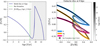 |
Fig. 1 Chemical evolution of inner Galactic disc at 4 kpc, computed with the same model parameters adopted in Spitoni et al. (2021), but using the stellar yields of Romano et al. (2010). Left panel: predicted age-metallicity relation highlighting the minimum [Fe/H] value after the bar formation (Age ≤ 8 Gyr). Right panel: evolution of abundance ratios [Fe/H] versus [X/Fe] (with X = Mg, Si, Ca). Large black-edged circles connected by a vertical green line indicate the predicted chemical composition of the ISM at the epoch of bar formation. |
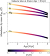 |
Fig. 2 Evolution of abundance by mass, X4D,i(t), of the elements considered in this study (i=Mg, Si, Ca, and Fe), as predicted by the model of the inner Galactic disc at 4 kpc after the formation of the Galactic bar (Age < 8 Gyr). |
2.2 The chemical-evolution model for the NSD
As indicated in the introduction, the NSD is primarily fuelled by gas channelled inwards by the Galactic bar from the inner disc regions. In this work, we refer to gas ‘flows’ generically without distinguishing between material originating in the disc and any possible residual contribution from other Galactic components. Our focus is on the chemical enrichment expected for the NSD, and in particular on constraining the degree of chemical preenrichment from the Galactic disc that is required to reproduce the available spectroscopic observations. We emphasise that our model assumes in situ formation for all NSD stars, whereas the gas reservoir feeding their formation may be supplied by the Galactic disc or other Galactic components. Hence, the equation of the evolution of the surface density of the chemical element i is
![Mathematical equation: $\[\dot{\sigma}_{N S D, i}=-\psi_{N S D}(t) X_{N S D, i}(t)+R_{N S D, i}(t)+\mathscr{F}_{N S D, i}(t)-W_{N S D, i}(t).\]$](/articles/aa/full_html/2026/03/aa58155-25/aa58155-25-eq4.png) (4)
(4)
The first term on the right-hand side of the equation accounts for the depletion of chemical elements from the ISM as they are locked into newly formed stars. Here, XNSD,i(t) denotes the abundance by mass of a given element, i; ψNSD is the SFR defined by the Kennicutt (1998) law of Eq. (2) with the same exponent, k, as the disc model and, ν, the star formation efficiency. The second term, RNSD,i(t), represents the fraction of matter that is restored to the ISM in the form of the element, i, originating from stellar winds and SN explosions. The ℱNSD,i quantity indicates the gas flow rate onto the NSD for the element i, and it can be written as
![Mathematical equation: $\[\mathscr{F}_{N S D, i}(t)=X_{\mathscr{F}, N S D, i}(t) \theta\left(t-\mathrm{T}_{\mathrm{bar}}\right) \mathscr{C} e^{-\left(t-\mathrm{T}_{\mathrm{bar}}\right) / \tau},\]$](/articles/aa/full_html/2026/03/aa58155-25/aa58155-25-eq5.png) (5)
(5)
which enforces that the NSD can only form after the onset of the bar. The latter is assumed to have developed Tbar = 8 Gyr ago, in agreement with Sanders et al. (2024). The parameter, 𝒞, is constrained by the total surface mass density of the NSD through this expression:
![Mathematical equation: $\[\mathscr{C}=\frac{\sigma_{N S D}}{\int_{\mathrm{T}_{\mathrm{bar}}}^{13.8 \mathrm{Gyr}} e^{-\left(t^{\prime}-\mathrm{T}_{\mathrm{bar}}\right) / \tau} d t^{\prime}},\]$](/articles/aa/full_html/2026/03/aa58155-25/aa58155-25-eq6.png) (6)
(6)
having imposed that the present-day total surface mass density, σNSD, of the NSD is
![Mathematical equation: $\[\sigma_{N S D}=\frac{5 \cdot 10^9}{\pi \cdot 100^2} \sim 5 \cdot 10^4\left[\mathrm{M}_{\odot} / \mathrm{pc}^2\right].\]$](/articles/aa/full_html/2026/03/aa58155-25/aa58155-25-eq7.png) (7)
(7)
In Eq. (7), we assumed that the radius of the NSD is RNSD = 100 pc and that its present-day total mass (gas plus stars) is 5 · 109 M⊙. Finally, the quantity Xℱ,NSD,i(t) represents the chemical composition of the gas that feeds the NSD. In Section 5.1, we present the different scenarios for the chemical composition of the gas inflowing into the NSD explored in this study. In addition, in Eq. (4) we assume the presence of a wind proportional to the SFR:
![Mathematical equation: $\[W_{N S D, i}(t)=\omega X_{N S D, i}(t) \psi_{N S D}(t),\]$](/articles/aa/full_html/2026/03/aa58155-25/aa58155-25-eq8.png) (8)
(8)
where ω is the loading factor.
2.3 Nucleosynthesis prescriptions
For both the inner Galactic disc and the NSD, we adopt the same set of stellar yields proposed by Romano et al. (2010, model 15). It is important to stress that this set was also used for the modelling of the Galactic bulge in Matteucci et al. (2019) and more recently to explain the new inner-bulge chemical-abundance data in the work of Nieuwmunster et al. (2023). For low – and intermediate – mass stars (0.8–8 M⊙), we adopted the metallicity-dependent yields of Karakas (2010), which include the contribution of thermal pulses. For massive stars (with masses ≳11–13 M⊙, depending on the explosion energy), which give rise to either Type II supernovae or hypernovae, we adopted metallicity-dependent He, C, N, and O yields computed with the Geneva evolutionary models that include the combined effects of stellar rotation and mass loss (Meynet & Maeder 2002; Hirschi 2005, 2007; Ekström et al. 2008). For the elements heavier than oxygen, we used the stellar yields calculated by Kobayashi et al. (2006).
3 Data sample for the NSD metallicity distribution
The models presented in this work will be constrained by the MDF derived from an updated stellar sample of candidate NSD members originally presented by Schultheis et al. (2021). In Schultheis et al. (2021), they presented the kinematics and global metallicities for NSD candidates based on the observations of K–M giant stars via a dedicated KMOS (VLT, ESO) spectroscopic survey.
We call Sample A the same sub-sample of stars used in Sormani et al. (2022) to construct self-consistent dynamical models of the NSD. These authors used a preliminary version of the second version of the Via Lactea survey Infrared Astrometric Catalogue (VIRAC2, Smith et al. 2025) to exclude stars that had large errors on proper motions. Here, we did not use the proper motions, we simply selected the same sample of stars for consistency. By simultaneously modelling the contamination from the Galactic bar with an N-body simulation, Smith et al. (2025) were able to assign posterior membership probabilities to individual stars, thereby providing a robust probabilistic framework for the identification of genuine NSD members. Sample A comprises 1806 stars. In Fig. 3, the MDF in terms of [Fe/H] for this sample is shown via filled pink histograms. As anticipated in Section 2.2, the MDF of the selected NSD stars covers a wide metallicity range, from −1.44 dex to 0.95 dex in [Fe/H], with a median value of [Fe/H]median = 0.08 dex. In Sample A, we find that ~22% of the stars have total velocities exceeding vtot > 250 km s−1. These high velocities are characteristic of bulge populations, and the derived fraction should be regarded as a conservative lower limit.
Hence, we also considered another sample to minimise the contamination of NSD disc stars by the Galactic bulge. From Figure 13 of Schultheis et al. (2021), it can be seen that the correlation between metallicity and velocity dispersion overlaps with that of the Galactic bulge for metallicities below [M/H] < −0.3/−0.5 dex, indicating a high level of bulge contamination. To account for this possibility, we defined a second sub-sample starting from Sample A by excluding all stars with [Fe/H] < −0.3 dex (Sample B). Sample B is composed of 1544 stars.
4 Fitting procedure with MCMC methods
Here, we present the main characteristics of the Bayesian analysis based on MCMC methods adopted in this work. In Section 4.1, we introduce the adopted likelihood, and in Section 4.2 we introduce the parameter priors and the MCMC sampling procedure.
4.1 Likelihood definition
Bayesian analysis based on MCMC methods has transformed scientific research in the past decade. Since several textbooks and reviews of Bayesian statistics (see e.g. Jaynes 2003; Gelman et al. 2013) and MCMC methods (see e.g. Brooks et al. 2011; Sharma 2017; Hogg & Foreman-Mackey 2018; Speagle 2019) already exist, we only summarise the general framework and highlight the aspects specific to the problem at hand. In the context of Galactic chemical evolution, Bayesian inference and MCMC techniques have already proven extremely effective in constraining the parameter space of chemical evolution models for the Galactic disc (Spitoni et al. 2020, 2021) and dwarf galaxies (Côté et al. 2017; Johnson et al. 2023; Plevne & Akbaba 2025), motivating their use for the present NSD study.
In parameter estimation, Bayes’ theorem provides a way to update the probability of the model parameters based on newly available data. It enables the calculation of the posterior probability distribution of the parameters given the data,
![Mathematical equation: $\[P(\boldsymbol{\Theta} {\mid} \mathbf{x})=\frac{P(\boldsymbol{\Theta})}{P(\mathbf{x})} P(\mathbf{x} {\mid} \boldsymbol{\Theta}),\]$](/articles/aa/full_html/2026/03/aa58155-25/aa58155-25-eq9.png) (9)
(9)
where x represents the set of observables, Θ the set of model parameters, P(x|Θ) ≡ ℒ the likelihood (i.e. the probability of observing the data given the model parameters), P(Θ) the prior (i.e. the probability of the model parameters before considering the data), and P(x) the evidence (i.e. the total probability of the data under all possible parameter values). The evidence is a normalising constant obtained by integrating the likelihood over the full parameter space.
In the present work, the observables are given by the spectroscopic data already described in Section 3 for the NSD, for example x = {[Fe/H]}, while the free parameters are those defining the chemical-evolution models, Θ = {τ, ν, ω}; these are, namely, the infall timescale, star formation efficiency, and wind loading factor, respectively. They were explored using MCMC sampling, and their posterior distributions were constrained by the observed MDF and abundance-ratio trends of NSD stars.
To identify the best-fitting chemical evolution models, we adopted a Bayesian framework employing MCMC techniques, following the methodology outlined in Spitoni et al. (2020) and applied to the MDFs (Cescutti et al. 2020). Below, we summarise the main elements of the fitting procedure; further methodological details can be found in the aforementioned works.
To evaluate the likelihood, ℒ, of a given chemical-evolution model with respect to the observed metallicity-distribution function (MDF), we proceeded as follows. We applied a Gaussian smoothing to the normalised predicted MDF to account for observational uncertainties (MDFModel smooth). The width of the smoothing kernel was set to σ[Fe/H]=0.2 dex and was consistent with the sample errors. The predicted MDFModel smooth was then interpolated using a one-dimensional linear spline function (MDFModel smooth(fit)). The observational data consisted of individual stellar [Fe/H] measurements. The log-likelihood was then calculated as the sum of the logarithms of the interpolated MDF evaluated at each observed metallicity:
![Mathematical equation: $\[\log~ \mathscr{L}=\sum_{i=1}^N ~\log~ \left[\mathrm{MDF}_{\text {Model smooth(fit) }}\left([\mathrm{Fe} / \mathrm{H}]_{\text {obs.}, i}\right)\right],\]$](/articles/aa/full_html/2026/03/aa58155-25/aa58155-25-eq10.png) (10)
(10)
where N is the number of stars in the observed sample. This log-likelihood function was used within the MCMC framework to constrain the posterior distribution of the model parameters.
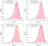 |
Fig. 3 Comparison between observed NSD MDF (Sample A, filled distributions; see Section 3 for details) and the predictions of the best-fit models (with parameters listed in Table 1), after applying a Gaussian convolution with σ[Fe/H]=0.2 dex (‘Model smooth’). The analytical fit to this distribution, indicated as ‘smooth (fit)’ in the likelihood definition of Eq. (10), is also shown. |
4.2 Parameter priors and MCMC sampling procedure
Uniform priors were adopted for all model parameters. The infall timescale, τ, is allowed to vary within 0.1 < τ < 10 Gyr. The wind-loading factor, ω, which regulates the strength of galactic outflows, is sampled uniformly in the 0 < ω < 10 range. The star formation efficiency, ν, was explored over the interval 0.1 < ν < 100 Gyr−1. These intervals ensured a comprehensive exploration of parameter space, covering the typical values adopted in chemical-evolution models of a wide variety of systems –including bulges, galactic discs, and dwarf and irregular galaxies– as discussed by Matteucci (2021).
The posterior distributions were sampled using the Affine invariant MCMC ensemble sampler, ‘emcee: the mcmc hammer’ code1, proposed by Goodman & Weare (2010) and Foreman-Mackey et al. (2013). This method allows for efficient exploration of high-dimensional parameter spaces and is well suited to problems involving complex, multi-modal distributions. We initialised the chains with 14 walkers and ran the sampler for 2800 steps. The computations were performed on the LEONARDO Data Centric General Purpose (DCGP) of CINECA, using 42 cores and 24 GB of memory.
5 Results for the NSD chemical evolution
In this section, we present the main results of our chemical evolution models for the NSD, obtained within the Bayesian MCMC framework described in Section 4 and constrained by the MDFs derived from Sample A and Sample B, as introduced in Section 3. In Section 5.1, we first present the different models characterised by different degrees of chemical dilution in the inflowing gas from the inner disc. In Section 5.2, we discuss the best-fit model parameters as inferred from the MCMC analysis. In Section 5.3, we compare these best-fit models with additional observational constraints, including the star formation history estimated by Sanders et al. (2024). Finally, in Section 5.4, we confront the model predictions with abundance ratios as reported by Ryde et al. (2025).
5.1 Chemical composition of the inflowing gas into the NSD
The observed MDF of the Sample A in Fig. 3 exhibits a significant sub-solar metallicity tail, extending from [Fe/H] ~ −1.2 to 0 dex. In contrast, the chemical composition of the inner Galactic disc at the time of bar formation (~8 Gyr ago), as presented in Section 2.1, is already close to solar value ([Fe/H]=−0.10 dex). Therefore, in this case, a scenario in which the NSD is built solely from disc gas cannot account for the sub-solar metallicity component of the MDF.
In the Bayesian framework (see Section 4), the MDF will be used as observational data to be reproduced by the model. This requires considering a certain level of dilution in the inflowing gas. In this study, we investigated different levels of chemical enrichment for Xℱ,NSD,i(t) in order to assess which degree of dilution provides the most consistent reproduction of the observed metallicity distribution of stars in the NSD.
Using as a constraint the NSD stars of Sample A, we explored four different prescriptions for the chemical composition of the gas inflowing into the NSD, Xℱ,NSD,i(t), and summarised as
![Mathematical equation: $\[X_{\mathscr{F}, N S D, i}(t)=\left\{\begin{array}{ll}\text { Primordial, } & \text { Model PRIM } \\X_{4 D, i}(t) / 10, & \text { Model ENR_D10 } \\X_{4 D, i}(t) / 5, & \text { Model ENR_D05 } \\X_{4 D, i}(t) / 3, & \text { Model ENR_D03 }\end{array}.\right.\]$](/articles/aa/full_html/2026/03/aa58155-25/aa58155-25-eq11.png) (11)
(11)
In the first case (Model PRIM), the accreting gas is assumed to be primordial, representing an extreme scenario. In the other three models, the inflow is considered to be partially enriched in a self-consistent manner by the inner Galaxy as a function of evolutionary time, but only for epochs successive to the formation of the bar. Specifically, the enrichment level is scaled down by a factor of 10 (ENR_D10), 5 (ENR_D05), or 3 (ENR_D03) with respect to the chemical composition of the disc gas, X4D(t). These prescriptions enabled us to explore the effect of different degrees of pre-enrichment on the resulting metallicity distribution of the NSD.
The fact that the gas forming the NSD should be less metal rich than the gas coming from the inner disc can be explained by the addition of more metal poor gas originating from the early formation of the bulge or thick disc (see also Ryde et al. 2025). Moreover, in a recent study Sextl & Kudritzki (2025) analysed the nuclear star-forming rings of four disc galaxies (NGC 613, NGC 1097, NGC 3351, and NGC 7552). By separating the spectral contributions of young and old stellar populations, they identified a wide range of ages and metallicities among the oldest stars in these nuclear rings. This diversity suggests a continuous inflow of metal-poor gas and recurrent episodes of star formation occurring over several Gyr.
Finally, we performed an additional test using the MDF of Sample B (see Section 3), excluding stars with [Fe/H] < −0.3 dex. In this specific case, we adopted an NSD model in which the chemical composition of the accreted gas is assumed to be identical to that of the inner Galactic disc as a function of time, i.e. Xℱ,NSD,i(t) = X4D,i(t). We refer to this model as Model ENR.
5.2 Results of the MCMC analysis
Figure 4 displays the posterior probability density functions (PDFs) of the three free parameters of our chemical evolution models for the NSD, which were obtained using Sample A as the observational constraint: the infall timescale (τ), the windloading factor (ω), and the star formation efficiency (ν). Figure 4 was generated using the final 800 iterations of the chains after discarding the burn-in phase. With a mean auto-correlation time of τencee ~ 48 for the four models considered, the 2800 iterations performed were sufficient to ensure chain convergence. The median values and 1σ confidence intervals are summarised in Table 1.
A consistent outcome across all models is that the NSD wind-loading factor is very low, with typical values around ω ≃ 0.01. This indicates that outflows have played a negligible role in shaping the chemical evolution of the NSD, consistent with the deep gravitational potential in which it is embedded.
The inferred infall timescales lie in the range of τ ≃ 4–5 Gyr and show little dependence on the assumed chemical composition of the inflowing gas (Fig. 5, black points). These values are consistent with predictions of the thin-disc component in the inner Galactic regions (Chiappini et al. 2001; Palla et al. 2020; Spitoni et al. 2021) By contrast, the star formation efficiency shows a strong dependence on the adopted enrichment prescription (Fig. 5, red points). Models with primordial or highly diluted inflows (PRIM and ENR_D10) require very high SFEs (ν ≳ 10 Gyr−1) comparable to those associated with the secular evolution of the bulge (Matteucci et al. 2019; Molero et al. 2024) in order to reproduce the observed MDF. In cases with moderate dilution (ENR_D05 and ENR_D03), the inferred values are instead closer to those typical of disc evolution in the inner Galactic regions (ν ≲ 5 Gyr−1).
To assess the relative quality of the chemical evolution models, we adopted the deviance information criterion (DIC), which provides a balance between the quality of the fit and the effective model complexity. In practice, the DIC was computed directly from the MCMC chains of the posterior probability. For each sampled parameter vector θ, we evaluated
![Mathematical equation: $\[\chi^2(\boldsymbol{\Theta})=-2 ~\log~ P(\boldsymbol{\Theta} {\mid} \mathbf{x}).\]$](/articles/aa/full_html/2026/03/aa58155-25/aa58155-25-eq12.png) (12)
(12)
From these values, the mean deviance and the minimum deviance were derived across the chain. The DIC was then estimated using the following expression:
![Mathematical equation: $\[\mathrm{DIC}=2\left\langle\chi^2\right\rangle-\min (\chi^2),\]$](/articles/aa/full_html/2026/03/aa58155-25/aa58155-25-eq13.png) (13)
(13)
where ⟨χ2⟩ denotes the mean over the posterior distribution and min(χ2) is the best-fit value found in the chain. The resulting DIC values allowed a direct comparison between the inflow scenarios considered in this work, with lower values indicating the statistically preferred model.
The relative performance of the four models is illustrated in Fig. 6, which shows their predicted DIC values. Model ENR_D03 provides the poorest fit, as indicated by its highest DIC value. This result is consistent with Fig. 3, where Model ENR_D03 clearly under-predicts stars in the low-metallicity tail of the MDF.
The next least favoured model is PRIM, which significantly overproduces stars in the metallicity range of −0.5 ≲ [Fe/H] ≲ 0, in clear disagreement with the observed MDF. By contrast, the best-fit model is ENR_D05, which achieves the lowest DIC value while accurately reproducing both the low-metallicity tail and the peak of the MDF. ENR_D10 offers an improvement over the primordial case. Taken together, these results indicate that the flowing gas that built the NSD must have been diluted relatively to the inner-disc composition by a factor approximately larger than three and smaller than ten. Pure inner-disc inflow is firmly ruled out. This suggests that, in addition to bar-driven inflows from the inner disc, lower-metallicity gas – possibly originating from the thick disc or from recent infall of pristine gas (Sextl & Kudritzki 2025) – also contributed to the NSD’s build-up.
As discussed in Section 5.1, in Model ENR we also explored the case where the chemical composition of the inflowing gas is identical to that of the inner disc. This configuration is only compatible with Sample B, where stars with [Fe/H] < −0.3 dex were excluded. For this analysis, we narrowed the prior parameter space for the Galactic outflow strength and star formation efficiency, guided by the best-fit results obtained for Sample A and restricting the ranges to 0 < ω < 10 and 0.1 < ν < 5 Gyr−1. Figure 7 shows that, in this case, the wind-loading factor of the best-fit model is no longer negligible, with ω = ![Mathematical equation: $\[1.959_{-1.222}^{+2.492}\]$](/articles/aa/full_html/2026/03/aa58155-25/aa58155-25-eq29.png) . Conversely, the best-fit star formation efficiency is quite low: ν =
. Conversely, the best-fit star formation efficiency is quite low: ν = ![Mathematical equation: $\[0.260_{-0.046}^{+0.185}\]$](/articles/aa/full_html/2026/03/aa58155-25/aa58155-25-eq30.png) Gyr−1. This outcome is consistent with the results obtained for Sample A, enforcing a chemically enriched inflow that drives the system towards reduced star formation, as a consequence of both stronger winds and lower star formation efficiency. We emphasise that in this study Sample B should be regarded as an extreme case, presented primarily to illustrate the only scenario in which an NSD model can be formed from gas inflow with inner-disc chemical composition, without any dilution.
Gyr−1. This outcome is consistent with the results obtained for Sample A, enforcing a chemically enriched inflow that drives the system towards reduced star formation, as a consequence of both stronger winds and lower star formation efficiency. We emphasise that in this study Sample B should be regarded as an extreme case, presented primarily to illustrate the only scenario in which an NSD model can be formed from gas inflow with inner-disc chemical composition, without any dilution.
We already discussed the fact that the low-metallicity gas required to dilute the inflow in the inner disc could originate either from the thick disc or from recent external accretion events. These two scenarios may be distinguished observationally through detailed chemical abundance patterns. The [Mg/Mn] versus [Al/Fe] diagram (Hawkins et al. 2015; Fernandes et al. 2023; Vasini et al. 2024) offers, in principle, a useful tool for distinguishing between these two scenarios because they are sensitive to different star formation histories. This sensitivity arises from the distinct nucleosynthetic origins and enrichment timescales of the elements involved. Mn is mainly released on long timescales by Type Ia SNe, which are also responsible for most of the iron production. In contrast, Mg and Al are primarily synthesised in massive stars and expelled into the interstellar medium by CC-SNe, which contribute only a minor fraction of the total iron budget. Thick-disc stars are known to exhibit enhanced relative [Al/Fe] and [Mg/Mn] ratios, reflecting their dominant enrichment by CC-SNe. On the other hand, gas accreted from the circumgalactic medium or from gas-rich satellites is expected to show lower [Al/Fe] and distinct [Mg/Mn] signatures due to slower chemical evolution and a larger contribution from Type Ia SNe. Future observations with MOONS will enable precise measurements of these abundance ratios and thus offer a valuable opportunity to distinguish between Galactic (thick-disc) and external (accretion-driven) origins of the metal-poor inflow. However, as emphasised by Vasini et al. (2024), the [Al/Fe]-[Mg/Mn] diagram remains theoretically uncertain. Its effectiveness as a diagnostic of star formation histories will critically depend on advances in stellar nucleosynthesis modelling for these elements, whose production mechanisms are still subject to substantial uncertainties.
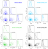 |
Fig. 4 Corner plots showing PDFs of the chemical-evolution model parameters for the different models reported in Table 1 (one in each panel). For each parameter, the median and the 16th and 84th percentiles of the posterior PDF are shown with dashed lines above the marginalised PDF. All models have adopted the Sample A data. |
Main properties of our best-fit models for the NSD varying the chemical enrichment of the gas flow.
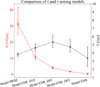 |
Fig. 5 Comparison of infall timescale, τ (red symbols and line, left-hand y-axis), and the star-formation efficiency, ν (black symbols and line, right-hand y-axis) for the different models reported in Table 1. |
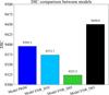 |
Fig. 6 Deviance information criterion (DIC) comparison between models in presence of gas dilution for the NSD. |
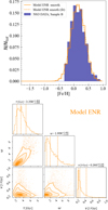 |
Fig. 7 Results of Model ENR. Upper panel: as in Fig. 3, but compared to the MDF obtained by using the Sample B (filled purple distribution; see Section 3 for details) and the predictions of the best-fit Model ENR (with parameters listed in Table 1). Lower panel: as in Fig. 4, but for Model ENR. |
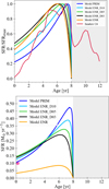 |
Fig. 8 Temporal evolution of star-formation rate (SFR) predicted by the NSD models listed in Table 1. Upper panel: SFR normalised to its maximum value and compared with the recent results of Sanders et al. (2024). Lower panel: SFR in physical units of M⊙ yr−1. The magenta point indicates the Henshaw et al. (2023) estimate of 0.1 M⊙ yr−1. In both panels, the grey shaded region marks the epoch preceding the formation of the Galactic bar. |
5.3 Comparison with other observational data
In addition to the MDF of NSD stars presented in Section 3, our models can also be compared with further observational constraints that are not directly included in the MCMC analysis. Figures 8–11 illustrate the predicted temporal evolution of the star formation rate, stellar mass, gas mass, and gas inflow rate for the four enrichment scenarios.
The predicted star formation histories in Fig. 8 show a pronounced enhancement of star formation immediately after the formation of the Galactic bar (about 8 Gyr ago), marking the onset of NSD formation. Stronger dilution scenarios lead to sharper peaks closer to this epoch, since a larger number of stars must form rapidly in order to reach the chemical enrichment level observed in present-day NSD stars.
The SFR estimated by Sanders et al. (2024) and drawn in the upper panel of Fig. 8 shows a rapid decline in recent times, approaching a near-zero value, while all other proposed models exhibit a less pronounced decrease, retaining 20–45% of their peak levels at present. It is important to stress that Sanders et al. (2024) derived the NSD star formation history from MIRA variables used as age tracers. These evolved stars provide strong constraints on ancient star formation episodes (around 8 ± 1 Gyr ago), but they are less sensitive to very recent activity. This limitation likely explains the almost negligible star formation at the most recent epochs in their reconstruction, in contrast with our models, which predict a more extended star formation history.
The star formation history inferred by Sanders et al. (2024) also shows a modest component prior to the epoch of bar formation. As already highlighted in previous sections, in our modelling we assume that the NSD formed only after the establishment of the Galactic bar (Baba & Kawata 2020; Cole et al. 2014). We interpret the small pre-bar component in Sanders et al. (2024) reconstruction as likely spurious, or the result of contamination from the surrounding bulge-and-Galactic-bar system.
In the lower panel of Fig. 8, we show the temporal evolution of the SFR, expressed in units of M⊙ yr−1, as predicted by our models with different dilution levels. Our results for models including gas dilution (i.e. those constrained by Sample A) are in good agreement with the estimated present-time star formation rate of 0.1 M⊙ yr−1 reported by Henshaw et al. (2023). Among these, the PRIM model provides the best agreement, whereas the other cases predict values in the range 0.12–0.14 M⊙ yr−1. Conversely, the model without dilution (Model ENR) constrained by Sample B substantially underestimates the Henshaw et al. (2023) value, predicting a rate of only 0.032 M⊙ yr−1.
The predicted build-up of stellar mass (see Fig. 9) is broadly consistent with estimates of the present-day NSD mass of ~109 M⊙. Our models based on Sample A slightly overestimate this value, with predictions ranging from 1.15 × 10⁹ M⊙ (Model ENR_D03) to 1.35 × 10⁹ M⊙ (Model PRIM). On the other hand, Model ENR, based on the Sample B, underestimates the present-day stellar mass, predicting a value of 3.14 × 10⁸ M⊙.
In Fig. 10, we also present the predicted evolution in time of the gas mass by different models. As reference we used the estimated value observed for the CMZ of 2–6 × 10⁷ M⊙ (Dahmen et al. 1998; Ferrière et al. 2007). We can notice that only models PRIM and ENR_D10 fall into this observed range. Models with lower dilution tend to overestimate the present-day gas mass. In fact, since fewer stars are needed to reproduce the observed MDF as indicated in Fig. 9 (due to the higher chemical enrichment of the infalling gas), the system is left with more gas. On the same line, Model ENR, where no chemical dilution of the inflowing gas is considered, gives a value of 2.90 × 10⁸ M⊙.
Finally, Fig. 11 shows the temporal evolution of the gas inflow rate predicted by the models, extended to the entire region occupied by the CMZ. This is computed by adopting the same total surface mass density as in Eq. (7), multiplied by the area ![Mathematical equation: $\[\pi R_{\mathrm{CMZ}}^{2}\]$](/articles/aa/full_html/2026/03/aa58155-25/aa58155-25-eq32.png) with RCMZ = 150 pc. The pink point with error bars corresponds to the estimate of Hatchfield et al. (2021), obtained from hydrodynamic simulations with AREPO. All model predictions lie below the 1σ Hatchfield et al. (2021) estimate. The best agreement with the data is obtained for Model ENR_D05.
with RCMZ = 150 pc. The pink point with error bars corresponds to the estimate of Hatchfield et al. (2021), obtained from hydrodynamic simulations with AREPO. All model predictions lie below the 1σ Hatchfield et al. (2021) estimate. The best agreement with the data is obtained for Model ENR_D05.
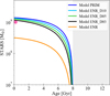 |
Fig. 9 As in Fig. 8, but for the evolution of the total stellar mass predicted by the models. The magenta point indicates the estimated present-day total stellar mass for NSD of 109 M⊙ (Launhardt et al. 2002; Nogueras-Lara et al. 2020; Schultheis et al. 2025). |
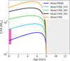 |
Fig. 10 Same as Fig. 8, but showing the evolution of the gas mass predicted by the models. The pink area indicates the range of the estimated mass of the molecular gas of the CMZ (Dahmen et al. 1998; Ferrière et al. 2007). |
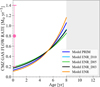 |
Fig. 11 Temporal evolution of inflow gas rate predicted by the models extended for the whole CMZ region, assuming the same total surface mass density of Eq. (7) and multiplied by an area of |
![Mathematical equation: $\[\pi R_{C M Z}^{2}\]$](/articles/aa/full_html/2026/03/aa58155-25/aa58155-25-eq31.png)
5.4 Comparison with Ryde et al. (2025) abundance ratios
In Fig. 12, we compare the predicted [Mg/Fe], [Si/Fe], and [Ca/Fe] versus [Fe/H] abundance ratios with the recent high-resolution measurements of NSD giants by Ryde et al. (2025). Concerning all models based on the Sample A (see Section 3), it is important to note that while all of them reproduce the overall behaviour of the data, the case with purely primordial infall (PRIM) is physically unrealistic, since some chemical enrichment from the inner disc is expected in the NSD. Consistently with this notion, the MCMC analysis already indicated that Model PRIM provides the statistically second poorest fit to the observations. By contrast, the ENR_D10 and ENR_D05 models, which also yield a good agreement with the observed MDF (see Fig. 6), successfully reproduce the observed decline of [α/Fe] with increasing metallicity, thereby supporting the requirement of a significant dilution level in the accreted gas. Taken together, the MDF of the full dataset (Sample A) and abundance-ratio comparisons demonstrate that the NSD cannot be explained by the accretion of chemically evolved inner-disc gas alone. Its formation must have involved a substantial contribution of lower-metallicity material, plausibly originating in the thick disc or the Galactic halo. Model ENR, calibrated on the MDF of Sample B stars, exhibits the smallest evolution in the [Fe/H]-[α/Fe] plane and only reproduces the four super-solar metallicity stars reported by Ryde et al. (2025). Since the work of Ryde et al. (2025) may have been contaminated by bulge stars, this scenario cannot be ruled out, but further analyses with larger datasets will be needed to confirm these results.
An additional comparison can be drawn with the chemodynamical models of Friske & Schönrich (2025). In their Figures 6 and 7, the predicted gas-phase abundance-ratio trends exhibit a markedly irregular behaviour, in contrast to the smooth [α/Fe]-[Fe/H] sequences observed by Ryde et al. (2025), which were reproduced well by our models. Furthermore, the models of Friske & Schönrich (2025) did not generate NSD stars with metallicities below [Fe/H] ≃ −0.1 dex, whereas such metal-poor stars are clearly present in the Ryde et al. (2025) sample and are naturally accounted for by our diluted inflow scenarios.
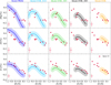 |
Fig. 12 Comparison between model predictions and NSD data from Ryde et al. (2025, red points). Each panel shows the evolution of [Mg/Fe], [Si/Fe], and [Ca/Fe] as a function of [Fe/H], as predicted by the four chemical-evolution models considered in this work (PRIM, ENR_D10, ENR_D05, and ENR_D03; see Table 1 for the adopted parameters). Shaded regions around the model curves indicate the uncertainties obtained by Gaussian smoothing with σ[Fe/H] = 0.2 dex (this is consistent with the MDF fitting procedure) and σ[X/Fe] = 0.1 dex, where X denotes the considered element. Typical uncertainties of the Ryde et al. (2025) data are indicated in the lower left corner of each panel by a red cross. |
6 Conclusions
In this work, we developed the first dedicated chemical-evolution models of the Milky Way’s NSD, employing a Bayesian framework to fit the observed MDF derived from various sub-samples of the Schultheis et al. (2021) dataset, as described in Section 3. Our main results can be summarised as follows:
For models compared to Sample A (full MDF with the low-metallicity tail), we find that a scenario in which the NSD forms exclusively from gas originating in the inner Galactic disc is inconsistent with the observed MDF. By the time the Galactic bar formed (~8 Gyr ago), the metallicity of the inner disc had already reached nearly solar values. As a result, such models cannot account for the sub-solar metallicity wing of the MDF observed in this NSD stellar sub-sample of Schultheis et al. (2021);
A certain level of dilution of the inflowing gas is required. The best-fit models correspond to inflows enriched to roughly one-fifth of the inner disc metallicity (ENR_D05), with an accretion timescale of τ =
![Mathematical equation: $\[5.324_{-0.655}^{+0.872}\]$](/articles/aa/full_html/2026/03/aa58155-25/aa58155-25-eq33.png) Gyr, a relatively high star-formation efficiency of ν =
Gyr, a relatively high star-formation efficiency of ν = ![Mathematical equation: $\[4.041_{-0.473}^{+0.733}\]$](/articles/aa/full_html/2026/03/aa58155-25/aa58155-25-eq34.png) Gyr−1, and a negligible wind-loading factor (ω =
Gyr−1, and a negligible wind-loading factor (ω = ![Mathematical equation: $\[0.008_{-0.006}^{+0.013}\]$](/articles/aa/full_html/2026/03/aa58155-25/aa58155-25-eq35.png) );
);The DIC comparison clearly favours the ENR_D10 and ENR_D05 models (inflows enriched to one-tenth and one-fifth of the inner disc metallicity, respectively), while the primordial (PRIM) and weakly diluted (ENR_D03) models are disfavoured;
For Model ENR applied to Sample B (stars with [Fe/H] < −0.3 dex were excluded), assuming that the inflowing gas has the same composition as the inner disc, the best-fit solution implies a significant wind (ω =
![Mathematical equation: $\[1.959_{-1.222}^{+2.492}\]$](/articles/aa/full_html/2026/03/aa58155-25/aa58155-25-eq36.png) ) and a low star formation efficiency (ν =
) and a low star formation efficiency (ν = ![Mathematical equation: $\[0.260_{-0.046}^{+0.185}\]$](/articles/aa/full_html/2026/03/aa58155-25/aa58155-25-eq37.png) Gyr−1). This is consistent with Sample A results, showing that chemically enriched inflows tend to suppress star formation through stronger winds and reduced efficiency;
Gyr−1). This is consistent with Sample A results, showing that chemically enriched inflows tend to suppress star formation through stronger winds and reduced efficiency;The predicted star formation histories of the best-fit models show a prolonged period of activity after bar formation, in agreement with independent constraints from stellar-population studies (Sanders et al. 2024);
The models tailored to Sample A also successfully reproduce the observed [α/Fe]–[Fe/H] trends of Ryde et al. (2025), whereas the Model ENR (based on Sample B) is only able to trace the four super-solar metallicity stars reported by Ryde et al. (2025).
These results suggest that, in addition to bar-driven inflows enriched by the inner disc’s lower metallicity gas – possibly originating from the Galactic thick disc or from recent infall of gas (Sextl & Kudritzki 2025) – also could have played a significant role in the build-up of the NSD.
Future spectroscopic surveys with large multiplex instruments such as MOONS will vastly increase the available sample of NSD stars with high-quality abundances. Further studies, focusing on stellar kinematics and chemical abundances, are needed to assess bulge contamination in NSD sample stars and, hence, to constrain the maximum dilution required by the model to reproduce the observations. Combined with the Bayesian framework developed here, these data provide stringent tests of the NSD formation scenario and offer new insights into the assembly of the Milky Way’s central regions.
Acknowledgements
The authors are grateful to the referee for the helpful suggestions that contributed to improving the clarity and quality of the manuscript. E.S. thanks R. Ingrao and A. Vasini for the very useful discussions. E.S., F.M. and G.C. thank I.N.A.F. for the 1.05.24.07.02 Mini Grant – LEGARE “Linking the chemical Evolution of Galactic discs AcRoss diversE scales: from the thin disc to the nuclear stellar disc” (PI E. Spitoni). We thank Leonardo-DCGP supercomputer as part of the INAF Pleadi Call 6. E.S and G.C. thank I.N.A.F. for the 1.05.23.01.09 Large Grant – Beyond metallicity: Exploiting the full POtential of CHemical elements (EPOCH) (ref. Laura Magrini). F.M. thanks I.N.A.F. for the 1.05.12.06.05 Theory Grant – Galactic archaeology with radioactive and stable nuclei. F.M. thanks also support from Project PRIN MIUR 2022 (code 2022ARWP9C) “Early Formation and Evolution of Bulge and HalO (EFEBHO)” (PI: M. Marconi). M.C.S. acknowledges financial support from the European Research Council under the ERC Starting Grant “GalFlow” (grant 101116226) and from Fondazione Cariplo under the grant ERC attrattività no. 2023-3014. This work was also partially supported by the European Union (ChETECINFRA, project number 101008324). Supported by Italian Research Center on High Performance Computing Big Data and Quantum Computing (ICSC), project funded by European Union – NextGenerationEU – and National Recovery and Resilience Plan (NRRP) – Mission 4 Component 2 within the activities of Spoke 3 (Astrophysics and Cosmos Observations). B.T. acknowledges the financial support from the Wenner-Gren Foundation (WGF2022-0041).
References
- Ahumada, R., Allende Prieto, C., Almeida, A., et al. 2020, ApJS, 249, 3 [NASA ADS] [CrossRef] [Google Scholar]
- Asplund, M., Grevesse, N., Sauval, A. J., & Scott, P. 2009, ARA&A, 47, 481 [CrossRef] [Google Scholar]
- Athanassoula, E. 1992, MNRAS, 259, 345 [Google Scholar]
- Baba, J., & Kawata, D. 2020, MNRAS, 492, 4500 [NASA ADS] [CrossRef] [Google Scholar]
- Bittner, A., Sánchez-Blázquez, P., Gadotti, D. A., et al. 2020, A&A, 643, A65 [NASA ADS] [CrossRef] [EDP Sciences] [Google Scholar]
- Brooks, S., Gelman, A., Jones, G., & Meng, X.-L. 2011, Handbook of Markov Chain Monte Carlo (CRC press) [Google Scholar]
- Cescutti, G., Molaro, P., & Fu, X. 2020, Mem. Soc. Astron. Italiana, 91, 153 [NASA ADS] [Google Scholar]
- Chiappini, C., Matteucci, F., & Romano, D. 2001, ApJ, 554, 1044 [NASA ADS] [CrossRef] [Google Scholar]
- Cirasuolo, M., Fairley, A., Rees, P., et al. 2020, Messenger, 180, 10 [Google Scholar]
- Cole, D. R., Debattista, V. P., Erwin, P., Earp, S. W. F., & Roškar, R. 2014, MNRAS, 445, 3352 [NASA ADS] [CrossRef] [Google Scholar]
- Contopoulos, G., & Grosbol, P. 1989, A&ARev., 1, 261 [Google Scholar]
- Côté, B., O’Shea, B. W., Ritter, C., Herwig, F., & Venn, K. A. 2017, ApJ, 835, 128 [Google Scholar]
- Dahmen, G., Huttemeister, S., Wilson, T. L., & Mauersberger, R. 1998, A&A, 331, 959 [Google Scholar]
- Ekström, S., Meynet, G., Chiappini, C., Hirschi, R., & Maeder, A. 2008, A&A, 489, 685 [NASA ADS] [CrossRef] [EDP Sciences] [Google Scholar]
- Fernandes, L., Mason, A. C., Horta, D., et al. 2023, MNRAS, 519, 3611 [NASA ADS] [CrossRef] [Google Scholar]
- Ferrière, K., Gillard, W., & Jean, P. 2007, A&A, 467, 611 [NASA ADS] [CrossRef] [EDP Sciences] [Google Scholar]
- Foreman-Mackey, D., Hogg, D. W., Lang, D., & Goodman, J. 2013, PASP, 125, 306 [Google Scholar]
- Friske, J. K. S., & Schönrich, R. 2025, A&A, 701, A140 [NASA ADS] [CrossRef] [EDP Sciences] [Google Scholar]
- Gelman, A., Carlin, J., Stern, H., et al. 2013, Bayesian Data Analysis, 3rd Edn., Chapman & Hall/CRC Texts in Statistical Science (Taylor & Francis) [Google Scholar]
- Goodman, J., & Weare, J. 2010, Commun. Appl. Math. Computat. Sci., 5, 65 [Google Scholar]
- Grieco, V., Matteucci, F., Ryde, N., Schultheis, M., & Uttenthaler, S. 2015, MNRAS, 450, 2094 [NASA ADS] [CrossRef] [Google Scholar]
- Hatchfield, H. P., Sormani, M. C., Tress, R. G., et al. 2021, ApJ, 922, 79 [NASA ADS] [CrossRef] [Google Scholar]
- Hawkins, K., Jofré, P., Masseron, T., & Gilmore, G. 2015, MNRAS, 453, 758 [NASA ADS] [CrossRef] [Google Scholar]
- Henshaw, J. D., Barnes, A. T., Battersby, C., et al. 2023, in Astronomical Society of the Pacific Conference Series, 534, Protostars and Planets VII, eds. S. Inutsuka, Y. Aikawa, T. Muto, K. Tomida, & M. Tamura, 83 [Google Scholar]
- Hirschi, R. 2007, A&A, 461, 571 [NASA ADS] [CrossRef] [EDP Sciences] [Google Scholar]
- Hirschi, R. 2005, in From Lithium to Uranium: Elemental Tracers of Early Cosmic Evolution, 228, eds. V. Hill, P. Francois, & F. Primas, 331 [Google Scholar]
- Hogg, D. W., & Foreman-Mackey, D. 2018, ApJS, 236, 11 [NASA ADS] [CrossRef] [Google Scholar]
- Jaynes, E. T. 2003, Probability Theory: The Logic of Science (Cambridge: Cambridge University Press) [Google Scholar]
- Johnson, J. W., Conroy, C., Johnson, B. D., et al. 2023, MNRAS, 526, 5084 [NASA ADS] [CrossRef] [Google Scholar]
- Karakas, A. I. 2010, MNRAS, 403, 1413 [NASA ADS] [CrossRef] [Google Scholar]
- Kennicutt, Jr., R. C. 1998, ApJ, 498, 541 [Google Scholar]
- Kobayashi, C., Umeda, H., Nomoto, K., Tominaga, N., & Ohkubo, T. 2006, ApJ, 653, 1145 [NASA ADS] [CrossRef] [Google Scholar]
- Kroupa, P., Tout, C. A., & Gilmore, G. 1993, MNRAS, 262, 545 [NASA ADS] [CrossRef] [Google Scholar]
- Launhardt, R., Zylka, R., & Mezger, P. G. 2002, A&A, 384, 112 [NASA ADS] [CrossRef] [EDP Sciences] [Google Scholar]
- Matteucci, F. 2021, A&ARev., 29, 5 [Google Scholar]
- Matteucci, F., Grisoni, V., Spitoni, E., et al. 2019, MNRAS, 487, 5363 [Google Scholar]
- Meynet, G., & Maeder, A. 2002, A&A, 390, 561 [NASA ADS] [CrossRef] [EDP Sciences] [Google Scholar]
- Molero, M., Matteucci, F., Spitoni, E., Rojas-Arriagada, A., & Rich, R. M. 2024, A&A, 687, A268 [NASA ADS] [CrossRef] [EDP Sciences] [Google Scholar]
- Nieuwmunster, N., Nandakumar, G., Spitoni, E., et al. 2023, A&A, 671, A94 [NASA ADS] [CrossRef] [EDP Sciences] [Google Scholar]
- Nieuwmunster, N., Schultheis, M., Sormani, M., et al. 2024, A&A, 685, A93 [NASA ADS] [CrossRef] [EDP Sciences] [Google Scholar]
- Nogueras-Lara, F., Schödel, R., Gallego-Calvente, A. T., et al. 2020, Nat. Astron., 4, 377 [Google Scholar]
- Nogueras-Lara, F., Schödel, R., & Neumayer, N. 2021, ApJ, 920, 97 [NASA ADS] [CrossRef] [Google Scholar]
- Palla, M., Matteucci, F., Spitoni, E., Vincenzo, F., & Grisoni, V. 2020, MNRAS, 498, 1710 [Google Scholar]
- Plevne, O., & Akbaba, F. 2025, arXiv e-prints [arXiv:2508.14890] [Google Scholar]
- Romano, D., Karakas, A. I., Tosi, M., & Matteucci, F. 2010, A&A, 522, A32 [NASA ADS] [CrossRef] [EDP Sciences] [Google Scholar]
- Ryde, N., Nandakumar, G., Albarracín, R., et al. 2025, A&A, 699, A176 [NASA ADS] [CrossRef] [EDP Sciences] [Google Scholar]
- Sanders, J. L., Kawata, D., Matsunaga, N., et al. 2024, MNRAS, 530, 2972 [NASA ADS] [CrossRef] [Google Scholar]
- Schultheis, M., Fritz, T. K., Nandakumar, G., et al. 2021, A&A, 650, A191 [NASA ADS] [CrossRef] [EDP Sciences] [Google Scholar]
- Schultheis, M., Sormani, M. C., & Gadotti, D. A. 2025, A&ARev., 33, 7 [Google Scholar]
- Sextl, E., & Kudritzki, R.-P. 2025, arXiv e-prints [arXiv:2510.14757] [Google Scholar]
- Sharma, S. 2017, ARA&A, 55, 213 [Google Scholar]
- Smith, L. C., Lucas, P. W., Koposov, S. E., et al. 2025, MNRAS, 536, 3707 [NASA ADS] [CrossRef] [Google Scholar]
- Sormani, M. C., Sanders, J. L., Fritz, T. K., et al. 2022, MNRAS, 512, 1857 [CrossRef] [Google Scholar]
- Speagle, J. S. 2019, arXiv e-prints [arXiv:1909.12313] [Google Scholar]
- Spitoni, E., Silva Aguirre, V., Matteucci, F., Calura, F., & Grisoni, V. 2019, A&A, 623, A60 [NASA ADS] [CrossRef] [EDP Sciences] [Google Scholar]
- Spitoni, E., Verma, K., Silva Aguirre, V., & Calura, F. 2020, A&A, 635, A58 [NASA ADS] [CrossRef] [EDP Sciences] [Google Scholar]
- Spitoni, E., Verma, K., Silva Aguirre, V., et al. 2021, A&A, 647, A73 [EDP Sciences] [Google Scholar]
- Spitoni, E., Aguirre Børsen-Koch, V., Verma, K., & Stokholm, A. 2022, A&A, 663, A174 [NASA ADS] [CrossRef] [EDP Sciences] [Google Scholar]
- Spitoni, E., Matteucci, F., Gratton, R., et al. 2024, A&A, 690, A208 [NASA ADS] [CrossRef] [EDP Sciences] [Google Scholar]
- Thorsbro, B., Ryde, N., Rich, R. M., et al. 2020, ApJ, 894, 26 [NASA ADS] [CrossRef] [Google Scholar]
- Vasini, A., Spitoni, E., & Matteucci, F. 2024, A&A, 683, A121 [NASA ADS] [CrossRef] [EDP Sciences] [Google Scholar]
All Tables
Main properties of our best-fit models for the NSD varying the chemical enrichment of the gas flow.
All Figures
|
Fig. 1 Chemical evolution of inner Galactic disc at 4 kpc, computed with the same model parameters adopted in Spitoni et al. (2021), but using the stellar yields of Romano et al. (2010). Left panel: predicted age-metallicity relation highlighting the minimum [Fe/H] value after the bar formation (Age ≤ 8 Gyr). Right panel: evolution of abundance ratios [Fe/H] versus [X/Fe] (with X = Mg, Si, Ca). Large black-edged circles connected by a vertical green line indicate the predicted chemical composition of the ISM at the epoch of bar formation. |
| In the text | |
|
Fig. 2 Evolution of abundance by mass, X4D,i(t), of the elements considered in this study (i=Mg, Si, Ca, and Fe), as predicted by the model of the inner Galactic disc at 4 kpc after the formation of the Galactic bar (Age < 8 Gyr). |
| In the text | |
|
Fig. 3 Comparison between observed NSD MDF (Sample A, filled distributions; see Section 3 for details) and the predictions of the best-fit models (with parameters listed in Table 1), after applying a Gaussian convolution with σ[Fe/H]=0.2 dex (‘Model smooth’). The analytical fit to this distribution, indicated as ‘smooth (fit)’ in the likelihood definition of Eq. (10), is also shown. |
| In the text | |
|
Fig. 4 Corner plots showing PDFs of the chemical-evolution model parameters for the different models reported in Table 1 (one in each panel). For each parameter, the median and the 16th and 84th percentiles of the posterior PDF are shown with dashed lines above the marginalised PDF. All models have adopted the Sample A data. |
| In the text | |
|
Fig. 5 Comparison of infall timescale, τ (red symbols and line, left-hand y-axis), and the star-formation efficiency, ν (black symbols and line, right-hand y-axis) for the different models reported in Table 1. |
| In the text | |
|
Fig. 6 Deviance information criterion (DIC) comparison between models in presence of gas dilution for the NSD. |
| In the text | |
|
Fig. 7 Results of Model ENR. Upper panel: as in Fig. 3, but compared to the MDF obtained by using the Sample B (filled purple distribution; see Section 3 for details) and the predictions of the best-fit Model ENR (with parameters listed in Table 1). Lower panel: as in Fig. 4, but for Model ENR. |
| In the text | |
|
Fig. 8 Temporal evolution of star-formation rate (SFR) predicted by the NSD models listed in Table 1. Upper panel: SFR normalised to its maximum value and compared with the recent results of Sanders et al. (2024). Lower panel: SFR in physical units of M⊙ yr−1. The magenta point indicates the Henshaw et al. (2023) estimate of 0.1 M⊙ yr−1. In both panels, the grey shaded region marks the epoch preceding the formation of the Galactic bar. |
| In the text | |
|
Fig. 9 As in Fig. 8, but for the evolution of the total stellar mass predicted by the models. The magenta point indicates the estimated present-day total stellar mass for NSD of 109 M⊙ (Launhardt et al. 2002; Nogueras-Lara et al. 2020; Schultheis et al. 2025). |
| In the text | |
|
Fig. 10 Same as Fig. 8, but showing the evolution of the gas mass predicted by the models. The pink area indicates the range of the estimated mass of the molecular gas of the CMZ (Dahmen et al. 1998; Ferrière et al. 2007). |
| In the text | |
|
Fig. 11 Temporal evolution of inflow gas rate predicted by the models extended for the whole CMZ region, assuming the same total surface mass density of Eq. (7) and multiplied by an area of |
| In the text | |
|
Fig. 12 Comparison between model predictions and NSD data from Ryde et al. (2025, red points). Each panel shows the evolution of [Mg/Fe], [Si/Fe], and [Ca/Fe] as a function of [Fe/H], as predicted by the four chemical-evolution models considered in this work (PRIM, ENR_D10, ENR_D05, and ENR_D03; see Table 1 for the adopted parameters). Shaded regions around the model curves indicate the uncertainties obtained by Gaussian smoothing with σ[Fe/H] = 0.2 dex (this is consistent with the MDF fitting procedure) and σ[X/Fe] = 0.1 dex, where X denotes the considered element. Typical uncertainties of the Ryde et al. (2025) data are indicated in the lower left corner of each panel by a red cross. |
| In the text | |
Current usage metrics show cumulative count of Article Views (full-text article views including HTML views, PDF and ePub downloads, according to the available data) and Abstracts Views on Vision4Press platform.
Data correspond to usage on the plateform after 2015. The current usage metrics is available 48-96 hours after online publication and is updated daily on week days.
Initial download of the metrics may take a while.