| Issue |
A&A
Volume 707, March 2026
|
|
|---|---|---|
| Article Number | A258 | |
| Number of page(s) | 12 | |
| Section | Galactic structure, stellar clusters and populations | |
| DOI | https://doi.org/10.1051/0004-6361/202558333 | |
| Published online | 23 March 2026 | |
The Hubble Missing Globular Cluster Survey
II. Survey membership tools and kinematic analysis of NGC 6749
1
INAF – Astrophysics and Space Science Observatory of Bologna,
Via Gobetti 93/3,
40129
Bologna,
Italy
2
Department of Physics and Astronomy, University of Bologna,
Via Gobetti 93/2,
40129
Bologna,
Italy
3
INAF, Osservatorio Astronomico di Padova,
Vicolo dell’Osservatorio 5,
Padova
35122,
Italy
4
School of Mathematics and Physics, University of Queensland,
Brisbane,
Qld
4072,
Australia
5
Space Telescope Science Institute,
3700 San Martin Drive,
Baltimore,
MD
21218,
USA
6
atlanTTic, Universidade de Vigo, Escola de Enxeñaría de Telecomunicación,
36310
Vigo,
Spain
7
Universidad de La Laguna, Avda. Astrofísico Fco. Sánchez,
38205
La Laguna,
Tenerife,
Spain
8
INAF – Osservatorio Astronomico di Abruzzo,
Via M. Maggini,
64100
Teramo,
Italy
9
INFN – Sezione di Pisa, Università di Pisa,
Largo Pontecorvo 3,
56127
Pisa,
Italy
10
INAF – Osservatorio Astronomico di Roma,
Via Frascati 33,
00078
Monte Porzio Catone,
Roma,
Italy
11
INAF – Osservatorio Astrofisico di Arcetri,
Largo E. Fermi 5,
50125
Firenze,
Italy
12
Astrophysics Research Institute, Liverpool John Moores University,
146 Brownlow Hill,
Liverpool
L3 5RF,
UK
13
Institute for Computational Cosmology & Centre for Extragalactic Astronomy, Department of Physics, Durham University,
South Road,
Durham
DH1 3LE,
UK
★ Corresponding author: This email address is being protected from spambots. You need JavaScript enabled to view it.
Received:
1
December
2025
Accepted:
27
January
2026
Abstract
The Hubble Missing Globular Cluster Survey has secured high-quality astro-photometric data in two bands for 34 clusters never observed with HST. When combined with Gaia astrometry, this dataset enables the investigation of the bulk motion and the internal kinematics of these poorly studied clusters to an unprecedented level of detail. Focusing on the case of NGC 6749, we show that the quality of the combined Gaia-HST proper motions is sufficient to accurately assess the cluster stellar membership, determine its absolute proper motion with a precision superior to Gaia, and to investigate its kinematic profile for the first time. Proper motions were determined using the public code GAIAHUB, which for NGC 6749 combined datasets separated in time by ~8 years.The resulting measurements improve the precision of Gaia proper motions by a factor of 10 at the faint end and enabled us to recover the proper motion for 662 stars for which Gaia was only able to measure the positions. These proper motions efficiently decontaminate the colormagnitude diagram of NGC 6749 and made it possible to compare the efficacy of a method of statistical decontamination that only relies on the photometric information extracted from the HST parallel fields. Finally, using the sample of best-measured proper motions, we determined the velocity dispersion and anisotropy profiles of NGC 6749, which reveal an isotropic behavior in the inner cluster regions and a slight radial anisotropy outside 1.5 half-light radii. The proper motions and the code for statistically decontaminating the cluster’s color-magnitude diagram are made available as public products of the survey.
Key words: methods: data analysis / astrometry / proper motions / stars: kinematics and dynamics / globular clusters: individual: NGC6749
© The Authors 2026
 Open Access article, published by EDP Sciences, under the terms of the Creative Commons Attribution License (https://creativecommons.org/licenses/by/4.0), which permits unrestricted use, distribution, and reproduction in any medium, provided the original work is properly cited.
This article is published in open access under the Subscribe to Open model. This email address is being protected from spambots. You need JavaScript enabled to view it. to support open access publication.
1 Introduction
Globular clusters (GCs) are exceptional laboratories for understanding fundamental processes of galaxy formation and evolution (Searle & Zinn 1978). The system of the Milky Way (MW) GCs is no exception in this sense, as its chemical (see e.g., Recio-Blanco 2018; Horta et al. 2020; Monty et al. 2024; Ceccarelli et al. 2024), dynamical (e.g., Massari et al. 2019; Callingham et al. 2022; Chen & Gnedin 2024), and chronological (e.g., De Angeli et al. 2005; Marín-Franch et al. 2009; Dotter et al. 2010; Leaman et al. 2013; Massari et al. 2023) properties allow us to investigate the history of our Galaxy in detail.
Historically, the most fundamental advancements in the study of the system of the MW GCs came from observational campaigns of the Hubble Space Telescope (HST). The primary examples of these were the ACS Survey of Galactic Globular Clusters (Sarajedini et al. 2007), and the HST UV Legacy Survey of Galactic Globular Clusters (Piotto et al. 2015), which have shaped modern GC science. The latest example is the Hubble Missing Globular Cluster Survey (MGCS; HST Treasury Program GO-17435, PI: Massari), a campaign that has just been completed and that aims to provide homogeneous two-band photometry and astrometry for 34 GCs that have not been observed before with HST. The characteristics of the survey, the targets, and first results have been presented in Massari et al. (2025, Paper I, hereafter). There the authors showed that the high photometric precision achieved by the survey in the optical and near-IR bands enabled the determination of the age of two GCs with subgigayear precision. Paper I found that one of the two targets, 2MASS-GC01 (the highest-extincted GC currently known), might be the youngest GC known to date, even though its age of ~7 Gyr is so young as to question its nature as a genuine GC.
While the astro-photometric catalogs of all the 34 observed targets will be made publicly available with a forthcoming publication (Libralato et al., in prep.), this paper focuses on one cluster, namely NGC 6749, and describes its analysis by means of two techniques that are both crucial to achieve the objectives of the survey.
The first part of the investigation relies on measurements of the proper motions (PMs) for the stars in common in the HST MGCS and Gaia DR3 data (Gaia Collaboration 2023). PM-based kinematic analyses of GCs have flourished in the last decade through HST and Gaia. This astrometric Renaissance has greatly improved our understanding of GCs by clearly highlighting their kinematic complexity (Bianchini et al. 2018; Sollima et al. 2019; Vasiliev & Baumgardt 2021; Libralato et al. 2022; Watkins et al. 2022; Häberle et al. 2024; Dalessandro et al. 2024). Nevertheless, kinematic information is not always available for all GCs with HST or Gaia alone because of technical limitations such as crowding, extinction, distance (for Gaia), or simply the lack of sufficient multi-epoch data (for HST). The combination of HST and Gaia, however, has shown that it is possible to bypass some of these limitations and obtain PMs for the subsample of stars common to both catalogs (see e.g., Massari et al. 2018, 2020; del Pino et al. 2022; Bennet et al. 2024; Libralato et al. 2024). This opens new possibilities of studying additional systems that were rarely studied so far.
While the HST-Gaia duo provides a powerful new tool, this tool is not without its own limitations. Some of the goals of the MGCS survey, such as the determination of age, mass function, and binary fraction, require a clean sample of cluster stars spanning a wide range of magnitude and masses along the main sequence (MS). However, our HST images can observe objects that are fainter by 5-6 magnitudes than the Gaia limit. Consequently, relying on Gaia-HST (hereafter, GH) PMs alone would unavoidably lead to the loss of a significant fraction of objects along the faint MS of our target clusters. For this reason, we devised an additional analysis based on the statistical decontamination of the color-magnitude diagram (CMD), taking advantage of the simultaneous HST observations in the core and in an external field.
In this paper, we show the application of these two techniques to the case of NGC 6749, an in situ disk GC (Massari et al. 2019, eDR3 edition) located at a distance of 7.6 kpc (Baumgardt & Vasiliev 2021). It is a relatively massive GC with a half-mass relaxation time of ~2.5 Gyr (Baumgardt & Vasiliev 2021). Given the size of this GC (half-light radius of 66" Harris (1996), 2010 edition), we were able to map the kinematics of this cluster out to about two half-light radii with a single HST field in the core.
In Sect. 2 we present the dataset together with photometric calibration (Sect. 2.1) and the PM estimation (Sect. 2.2). Sect. 3 describes the two methods we used to infer membership probabilities of each star. One method uses GH PMs (Sect. 3.1), and the other focuses on the statistical approach (Sect. 3.2). In Sect. 4, we validate the model we used to study the PMs first with a mock catalog and then by comparing our results with the literature (Sect. 4.1). After the validation, we used the GH PMs to perform the radial kinematic analysis of NGC 6749 (Sect. 4.2), and we derived the physical properties through an N-body simulation comparison in Sect. 4.3. Finally, we summarize this work in Sect. 5.
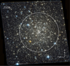 |
Fig. 1 Colored image of NGC 6749 using the new HST (ACS/WFC) observations. The white cross shows the center of the cluster (according to Baumgardt & Vasiliev 2021), and the radius of the white circle is equal to the half-light radius. |
2 Data reduction
We made use of the HST images of NGC 6749 taken within the MGCS on 2024 March 9-12. The dataset consists of four exposures (2 × 699 s, 1 × 337 s, and 1 × 30 s) per filter collected with the Wide Field Channel (WFC) of the Advanced Camera for Surveys (ACS) in the F606W and F814W bands on target, and of an analog set of parallel exposures with an identical setup using the Ultraviolet and Visible Instrument (UVIS) of the Wide Field Camera 3 (WFC3). The ACS/WFC data cover the central region of the cluster, as shown in Fig. 1, whereas the WFC3/UVIS parallel fields are off center by about 7 arcmin.
2.1 Photometry
This dataset was reduced as described in Massari et al. (2025), in accordance with the well-established prescriptions outlined in a number of papers presenting high-precision astrometry and photometry with HST images (Bellini et al. 2017; Nardiello et al. 2018; Libralato et al. 2018, 2022). We refer to Paper I and to the forthcoming paper by Libralato et al. for the details of the astro-photometric analysis. Briefly, the data reduction consists of two steps called first- and second-pass photometry. The first-pass photometry is used to create the initial astro-photometric catalogs, one for each HST image1. The positions and magnitudes in these catalogs were obtained via the software hst1pass2 (Anderson 2022a,b), which performs an effective-point-spread-function (ePSF) fit by means of the publicly available HST ePSF models, appropriately fine-tuned for each image. The positions are corrected for the effect of geometric distortion using publicly available corrections3. These first-pass catalogs are used to set up the astrometric and photometric reference systems for the second-pass photometry. The second-pass photometry is obtained with proprietary software KS2 (Anderson in prep.; Bellini et al. 2017), which analyzes all input images at once (thus enhancing the detection of faint sources) and is designed to overcome crowding-related limitations typical of environments such as GCs.
2.2 Astrometry
The astrometric analysis of NGC 6749 focuses on the central field observed with the ACS/WFC alone. The PMs of the stars in this region are computed by means of the publicly available tool GAIAHUB (del Pino et al. 2022). GAIAHUB combines HST and Gaia data to obtain PMs with a temporal baseline longer than that of the Gaia-DR3 PMs. As shown, for instance, by del Pino et al. (2022) and Bennet et al. (2024), GAIAHUB delivers PMs that can be more precise by one order of magnitude than those of Gaia at the Gaia faint end and in crowded environments.
GAIAHUB relies on astro-photometric catalogs computed for each HST image by means of the first-pass-photometry tool hst1pass, which is run in the background at the beginning of the process. To ensure a self-consistent infrastructure throughout our project, we modified GAIAHUB to use our first-pass astro-photometric catalogs (Sect. 2.1) instead of producing its own.
Before computing PMs, GAIAHUB transforms HST positions onto the reference frame of Gaia via a six-parameter linear transformation (two offsets, one rotation, one change of scale, and two skew terms4). In general, the coefficients of such transformations are computed by comparing two sets of positions of the same reference stars. If these positions are taken at different epochs, these transformations would map the different alignment between the frames and the actual motion of the reference stars between the two epochs. In our case, the latter contribution would bias our frame alignment because cluster and field stars have significantly different motions. To solve for this problem, we might either select a single group of stars (e.g., cluster stars, whose velocity dispersion and coherent motion would imprint a minimum contribution in the transformations), or propagate the positions of one of the two catalogs at the epoch of the other catalog (so that all stars can be used, regardless of the population to which they belong). We chose the latter option (using the –rewind_stars flag) to avoid a membership selection that at this stage might bias our PMs5, and to increase statistics.
The absolute PMs from GAIAHUB of the stars in the central field of NGC 6749 present a series of systematics as a function of position, magnitude, and color. We corrected for these systematic errors by comparing our GH PMs with those in the Gaia DR3 catalog. A detailed description of the systematic corrections is provided in Appendix A.
A comparison between our GH and the Gaia PMs is shown in Fig. 2. The top panels present the vector-point diagrams (VPDs) of the PMs in the Gaia DR3 catalog (left panel) and our PMs (middle and right panels). While the middle panel presents objects with a counterpart entry in the Gaia catalog, the right panel only includes sources without a PM in the Gaia catalog. The comparison of the VPDs for the same stars in our and Gaia panels (middle and left panels, respectively) already provides a qualitative assessment of the improvement brought by the HST - Gaia synergy, as the more populated clump in these diagrams (i.e., the distribution of the cluster stars) looks tighter with our PMs than with those in the Gaia DR3 catalog. This improvement in precision is more quantitatively shown in the two bottom panels in Fig. 2, where we compare the PM errors in each component of the motion as a function of G magnitude. At magnitudes fainter than G - 18.5, our PMs become more precise than the ones from Gaia by a factor of 3 and up to 10 at the very faint end, with a median value of δμ = 0.42 mas/yr for GH and δμ = 1.09 mas/yr for Gaia6. Furthermore, the GAIAHUB catalog contains PMs for 2634 stars compared to the 1972 from Gaia, incrementing by 662 the number of stars with this information. This de facto extends the astrometry to stars fainter by ~0.5 mag than in the Gaia catalog.
To reject poor measurements7, we applied the following criteria (Bellini et al. 2014; Libralato et al. 2018, 2022):
 (1)
(1)
where δμ is the PM error, and  is the local velocity dispersion measured using the n = 20 closest stars to each source (target excluded). Figure 3 shows the vector point diagram (VPD) and the CMD of NGC 6749. In the VPD, a tight clump of stars located at about (μαcosδ, μδ) = (−3, −5.5) mas yr−1 is embedded in other sources with a broader distribution. We selected stars within a radius of 1.0 mas yr−1 from the center of the tight clump (red circle) and plotted them in the CMDs (red dots in the middle panel). As expected, these are mainly cluster members (well aligned along the evolutionary sequences in the CMD), whereas the broadly distributed population in the VPD (those beyond the red circle in the left panel) comprises field stars along the line of sight of the cluster (black dots in the CMD). Zooming in around the CMD location of these stars (right panel), we can identify the cluster red giant branch (RGB) and horizontal branch (HB). In the following section, we address the problem of the cluster membership in a quantitative way using two different approaches.
3 Membership probability
We adopted two independent approaches to estimate the membership probability of the cluster sources detected in the MGCS images. The first approach only exploits the PM measurements, and the second approach only relies on the CMD comparison between the target and the WFC3/UVIS parallel observations. In Sections 3.1 and 3.2, we thoroughly describe each method, and in Sect. 3.3, we compare the two membership selections.
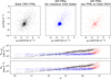 |
Fig. 2 Comparison between the Gaia and GH PMs. The top panels show the VPDs of the PMs, and the two bottom panels show the PM errors along α cos δ and δ as a function of Gaia G magnitude. The black dots refer to the Gaia PMs, and the blue and red dots show stars in our catalog with and without a corresponding PM in the Gaia catalog, respectively. |
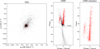 |
Fig. 3 VPD (left panel) and CMDs (middle and right panels) of NGC 6749 using the new HST data of the MGCS survey. The red circle with the radius of 1 mas yr−1 in the VPD was used to select likely cluster stars (those included within the circle). In the central CMD, the gray dots represent all stars in our HST photometric catalog, and the black and red dots are foreground and cluster stars, respectively, for which we have a PM measurements. The horizontal dashed line corresponds to the Gaia limiting magnitude. Finally, the right panel shows the location of cluster member stars in the CMD. |
3.1 Kinematic membership
The PM distributions of a GC and the background field often overlap significantly (Bellini et al. 2014; Libralato et al. 2022). This overlap complicates a clear-cut separation between members and nonmembers, which thereby necessitates a probabilistic approach. This approach assumes that the observed sample of stellar PMs is a realization of an underlying model. In its general form, this model consist of ncomp components, each corresponding to a distinct stellar population with its own kinematic structure and contributing to the global PM probability distribution P(μ),
 (2)
(2)
In the equation above, μ ≡ (μα cos δ,μδ), Pi(μ) is the probability distribution of each component, and wi represents its fractional contribution. We further required that
 (3)
(3)
to ensure a proper normalization. The model parameters were determined within a fully Bayesian framework by maximizing a well-motivated likelihood function of the data. When the parameters were determined, the model provided a probabilistic framework for assigning a membership probability to each star with respect to the different components.
In our specific application, we distinguished between two Gaussian components (i.e., a Gaussian mixture model; GMM): the target GC, and a term describing the foreground contamination (FG). Therefore, the model probability distribution (2) reduces to
 (4)
(4)
where GGC and GFG describe the PM distributions of the GC and the foreground stars, respectively, and w1 sets the relative contribution of the GC over the foreground.
We modeled each component as a bivariate Gaussian,
![Mathematical equation: G_i(\vec{\mu}) = \frac{\exp\big[{-}\frac{1}{2}(\vec{\mu}-\vec{\hat{\mu}}_i)^T\Sigma^{-1}_i(\vec{\mu}-\vec{\hat{\mu}}_i)\big]}{\sqrt{(2\pi)^2\det\Sigma_i}},](/articles/aa/full_html/2026/03/aa58333-25/aa58333-25-eq6.png) (5)
(5)
where  , and Σi are the center and the covariance matrix of the ith component, respectively, with i=GC or FG. The covariance matrix Σi is
 (6)
(6)
The model consists of the following free parameters, one per component (i=GC or FG):
μ̂i(α, δ) is the center of motion of each component.
σi(α, δ) is the standard deviation of each component.
ρi is the correlation between the standard deviation components.
w1 is the weight of the GC Gaussian in the mixture.
This is for a total of six free parameters.
The likelihood of the model for the observed dataset is
 (7)
(7)
where the product extends over the stars in our sample, the asterisk represents the convolution with the error function S, which is a bivariate Gaussian distribution with null mean, and the covariance is given by
 (8)
(8)
One of the great advantages of using Gaussians when describing multiple components in a mixture model is that the convolution between each model component and the error function is still a Gaussian with a mean and covariance matrix,  , given by the sums of the individual means and covariance matrices. In our specific case, the resulting covariance matrix can be written as
![Mathematical equation: \Sigma_i^{\rm obs}=\begin{pmatrix} (\sigma_{\alpha,i}^{\rm obs})^2 & \rho_i^{\rm obs}\sigma_{\alpha,i}^{\rm obs}\sigma_{\delta,i}^{\rm obs}\\[4pt] \rho_i^{\rm obs}\sigma_{\alpha,i}^{\rm obs}\sigma_{\delta,i}^{\rm obs}&(\sigma_{\delta,i}^{\rm obs})^2 \end{pmatrix},](/articles/aa/full_html/2026/03/aa58333-25/aa58333-25-eq12.png) (9)
(9)
where we called
 (10)
(10)
with  and
and
 (11)
(11)
In the above equations, i = GC or FG.
We determined the free model parameters using a Monte Carlo Markov chain (MCMC) method, relying on the EMCEE package (Foreman-Mackey et al. 2013). To sample the posterior and determine the model parameter confidence intervals, we ran an MCMC with 50 walkers, each evolved for 10 000 steps. We discarded the first 500 steps of each walker as burn-in and applied a thinning factor of 20, consistent with median value of the autocorrelation lengths of the free parameters, thereby ensuring a sample of effectively independent draws. The remaining steps were used to compute the distributions for the free model parameters. The median parameter values and any other derived quantity of the models were estimated as the 50th percentile of the corresponding distributions; the 1σ credible intervals were determined using the 16th and 84th percentiles of the distributions.
We assigned a membership probability to each star in the sample in the following way. For each star k, we computed the distribution of pk, that is, the probability of the kth star to belong the GC. This probability is defined as
 (12)
(12)
Consistently with credible interval estimates, we took as the probability the 50th percentile of the distribution. Figure 4 shows the VPD of NGC 6749 for 2184 stars using the new GH PMs, together with the marginal distributions the membership probability. As an example, the number of stars with a membership probability p > 0.8 is 1416.
3.2 Photometric membership
Even though the membership obtained from the PMs is more accurate, the kinematic information is only available for a limited number of stars. Another approach exploits the CMD to statistically infer the membership. When the photometric information is used, the number of suitable stars increases drastically. In the case of NGC 6749, we calculated the membership probability for 50 097 stars. This method requires the observation of a parallel field that is close enough to the target to be representative of the contaminating stellar population, but sufficiently far away to exclude GC members. Many algorithms have been proposed over the past 20 years to determine the membership in this way (e.g., Mighell et al. 1996; Knoetig 2014; Cabrera-Ziri et al. 2016). The general idea behind these algorithms is that the CMD of the field can be statistically subtracted from the CMD of the target GC. Some approaches defined a specific metric to evaluate the space nearby each star in order to understand its likelihood of being a contaminating star (e.g. Milone et al. 2018). Other algorithms implement a statistical subtraction to retrieve the membership probability. These approaches usually divide the CMD (the target and the parallel field) space in cells. For each cell, the information from the field CMD is used to perform a statistical subtraction in the same cell of the target CMD. Some implementations use a cell with a fixed size (Bonatto & Bica 2007; Dalessandro et al. 2019), while more recent works use adaptive grids. Our approach belongs to the latter case and works as follows. We tried to preserve the spatial resolution of the target CMD as much as possible while keeping a sufficient statistics per cell to avoid shot-noise bias. The grid was created via a Voronoi tesselation that naturally follows the stellar density in the CMD. Moreover, to ensure a uniform spatial distribution of contaminating stars (as we expect from a field population), we split the statistical subtraction into radial bins that always contained the same number of contaminants (see for example Dalessandro et al. 2019). At the beginning of the process, the membership was set to 1.0 for every star, and the following steps were then made to update the membership:
Creation of the Voronoi grid, based on the target CMD of the stars contained in the radial bin.
Dilation of the Voronoi grid. By design, the Voronoi grid creates a cell for each star. If we performed the following steps with only one star per cell, the final membership distribution would be biased by the shot noise. For this purpose, the Voronoi tesselation was dilated by merging the closest cells, starting from the smallest ones. This process was repeated until the distribution of the number of stars per cell had a median value equal to or greater than a desired threshold. We set a threshold of ten stars as the best trade-off between the loss of the grid resolution and a good statistics per cell8.
Count of the number of stars in the field CMD that fall in each cell, nfield.
Rescale nfield for the ratio of the field of view (FoV) of the parallel field (fovfield) and the sky area covered by the current radial bin (fovbin),
 .
.-
Convert nsub from a decimal into integer number with the following criteria:
![Mathematical equation: n_{sub}' = \begin{cases} \mathcal{B}([1 - n_{sub},\ n_{sub}]), & \text{if } n_{sub} < 1 \\ \text{int}(n_{sub}) + \mathcal{B}([1 - \text{dig}(n_{sub}),\,\text{dig}(n_{sub})]), & \text{if } n_{sub} \geq 1 \end{cases}\!\!,](/articles/aa/full_html/2026/03/aa58333-25/aa58333-25-eq18.png)
where int(nsub) and dig(nsub) are the mantissa and the decimal digits, respectively, and B is the Bernoulli distribution. In this way, we tried to take the decimal part of the normalized nsub into account.
For each cell, n′sub target stars were randomly subtracted. When n′sub was greater than the number of target stars within the cell, then all the stars were subtracted. This step was repeated many times (1000 in our case) to further mitigate the shot noise.
-
For each star, the membership was computed as follows:
 (13)
(13)where
 is the number of times that the ith star was subtracted, and
  is the total number of subtractions made in the jth cell that contains the star.
The process of statistical subtraction was combined with a differential reddening correction using the algorithm described in Milone et al. (2012). We iteratively combined the differential reddening correction and the statistical subtraction through the following algorithm:
The differential reddening correction of the target CMD was performed using as reference stars only those with a membership probability higher than a certain threshold (we used 90%). For the first iteration, all the stars were used because their membership probability is one.
We performed the statistical decontamination of the CMD using the differential reddening corrected magnitudes.
We iterated the two steps by updating the membership probabilities and the reddening correction.
We considered that the process reached convergence when the typical residual reddening corrections were on the order of the photometric error, which in this case was after three iterations. The result of our procedure is shown in Fig. 5. The top panels show the reddening-corrected CMDs of NGC 6749 and of its parallel field, respectively. From these, it is already evident that the overlap between the target main sequence (MS) and the field MS is quite strong, making this a challenging case for the statistical approach. The panel in the lower left corner shows the same target CMD, but color-coded based on the membership probability, which in turn is displayed in the lower right corner. The CMD of likely members appears to be very well defined, with likely contaminants populating the expected bluer and brighter sequence typically attributed to MW disk stars in the GC foreground or background. To give the same reference as for the kinematic membership in Section 3.1, the number of stars with p > 0.8 is 41 838.
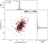 |
Fig. 4 Distribution of the NGC 6749 GH PMs. The central scatter plot shows the 2D VPD, where the points are color-coded by the membership probability obtained from the MCMC chains (color bar). The top and right histograms show the normalized marginal distributions of the PMs, together with the posterior distributions of the GMM components, the target in red, the field in blue, and their sum in gray. |
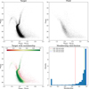 |
Fig. 5 Result of the statistical decontamination. (Top left panel) Contaminated target CMD. (Top right panel) Parallel field CMD. (Bottom left panel) Target CMD color-coded for the membership probability. (Bottom right panel) Membership probability distribution. The target CMDs were corrected for the differential reddening. |
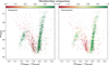 |
Fig. 6 Color-coded CMDs according to the membership probability. (Left) Membership calculated from the PMs. (Right) Membership obtained with the statistical approach. |
3.3 Comparison between the two methods
Using stars with both photometric and kinematic information, we directly compared the membership distributions obtained with the two methods described above. In Fig. 6 the target CMD is color-coded according to the membership probability obtained from the kinematic approach in the left panel and the photometric approach in the right panel. The two results are remarkably similar and thus demonstrate that the photometric procedure has worked successfully. For the sake of comparison, the 75% of stars with a kinematic membership p > 0.8 also have a photometric membership p > 0.8. Since this method will primarily be adopted by MGCS, for GCs with different properties, it is worth discussing some of the limitations that the statistical approach has compared to the kinematic approach. First, it is limited by the number of stars in the target CMD. In particular, few stars in the target CMD means a larger Voronoi cell size, which lowers the resolution and the ability to sample small and isolated features. Second, the dilation of the Voronoi cells at the edges of features such as the MS and the giant branches merges some of the small cells and maps the feature itself with the large cells that map the almost empty space next to it. As a result, these are more likely to be oversubtracted during the process. This mimics an erosion effect of the feature edges, where the membership probability is lower than in the inner parts. Finally, where no field signal is present in some cell (meaning that no stars are found in that cell in the field CMD), the membership is exactly one, while when the field signal dominates the target (i.e., when there are more field stars in that cell than the target stars), the membership drops to zero. However, the result shown in Figs. 5 and 6 suggests that our statistical approach is a valid method for decontaminating the entire target CMD. Therefore, we advice any user to select one method over the other depending on the needs of the specific science case of interest.
4 Kinematic analysis
By using the unprecedentedly precise PMs we measured and the GMM described in Section 3.1, we performed a detailed analysis of the internal kinematics of NGC 6749. First, we validated our approach in two ways: i) with a mock catalog with known parameters (see Section 4.1), and ii) with the Gaia DR3 PMs in the literature. After the validation, we refine in Section 4.2 the mean PM of the GC and build the first PM-dispersion radial profile for NGC 6749.
4.1 Validation with a mock catalog and external checks
We made a first validation of our GMM using a mock distribution of PMs, which qualitatively resembled the distribution shown in the VPD of NGC 6749, convolved with an error of 0.5 mas yr−1. Table 1 lsummarizes the comparison between the posterior distributions of the GMM parameters using the median value as reference and the 16th and 84th as uncertainties (i.e., the 1σ confidence range), and the parameters used to generate the mock distribution. The posterior distributions are always consistent within 1σ with the true input values, except for the mean motion of the cluster and the field along the declination (the μδ component), which are consistent with the input within 2σ, probably because in the shape of the VPD, the δ direction is most affected by the overlap between the cluster and the field component. However, this test shows that our GMM can successfully recover the properties of a PM distribution where the field and cluster components overlap strongly.
After the validation with the mock PMs, we tested our approach on the sample of member stars of NGC 6749 that were used to obtain the value of velocity dispersion quoted in Vasiliev & Baumgardt (2021). We remark that in this test (VB21 hereafter), we used a single-component GMM (i.e. a 2D Gaussian fit) because the sample consisted of member stars alone.
Figure 7 shows the comparison of the cluster mean motion components μα,δ and the PM dispersions σα,δ of the two PMs distributions. This figure shows that the μα,δ of the cluster component is well consistent between the two cases. Our measurement provides a mean PM of μα,δ = (−2.82, −5.99) mas yr−1, with a smaller uncertainty (0.008 mas yr−1)than VB21 (0.012mas yr−1). On the other hand, we find a larger discrepancy (at the 3σ level) in σδ, with our GH PMs providing σδ = 0.18 ± 0.01 mas yr−1, while for the VB21 sample, we determine σδ = 0.23 ± 0.01 mas yr−1.
To understand which of the two estimates is more realistic, we compared it with the current line-of-sight velocity dispersion values available for NGC 67499, that is,  km/s, as measured with a combination of Gaia DR3, Apogee DR19, and published literature RVs. Under the assumption of isotropy, our GH velocity dispersion estimates of σα = 6.83 km/s and σδ = 6.34 km/s (assuming a distance of 7.59 kpc, Baumgardt & Vasiliev 2021) agree better than those we obtained from VB21 of σα = 7.35 km/s and σδ = 8.11 km/s. This is reasonable evidence that our measurements led to an improved estimate of the cluster velocity dispersion. Our more precise GH PMs probably allow for a better deconvolution of cluster and field components in the GMM and thus enable a better selection of the actual stellar members. In passing, we also provide an estimate for the kinematic distance (dkin) of NGC 6749. Under the usual assumption of isotropy, the tangential velocity dispersion that we measured matches that along the line of sight for dkin = 6.92 ± 0.36 kpc, which is consistent within 1.2σ with the distance quoted by Baumgardt & Vasiliev (2021) of d = 7.59 ± 0.22 kpc.
Comparison between the posterior model distributions and the mock model.
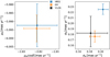 |
Fig. 7 Comparison of the mean velocity (left) and velocity dispersion (right) components for GH (orange), and GaiaDR3-VB21 (blue). The error bars are the 16th and 84th of the posterior parameter distribution. The current line-of-sight velocity dispersion (black) is shown as reference. |
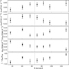 |
Fig. 8 Radial profiles of the mean velocity (μrad,tan), velocity dispersion (σrad,tan), and anisotropy (calculated as |

4.2 Kinematic analysis of NGC 6749
Based on the available large number of stars with measured PMs, we investigated the internal kinematics of NGC 6749. We divided our field into annular bins with a variable area, each containing at least 300 stars. We also decomposed our PMs from equatorial coordinates into their radial and tangential components to study features such as kinematic anisotropies and overall expansion and rotation in the plane of the sky. As we pointed out in Section 2.2, our GH PMs are more precise than Gaia’s at its faint end (G ≳ 18.5), while for brighter stars (G ≲ 18.5), Gaia is still the best option. For this reason, we decided to construct a golden sample of stars by selecting the PMs with the lowest uncertainty from either GH or Gaia. For each bin, we modeled the VPD using the GMM described in Section 3.1 by fixing the parameters of the field component to the median value of its posterior distribution, obtained using the golden sample. Figure 8 reports the radial trends of the cluster mean PM and PM dispersions along the radial and tangential directions σrad,tan. We also measured the ratio of the radial and tangential components of the velocity dispersion and thus obtained the anisotropy profile of NGC 6749. The trend of the mean GC motion as a function of radius can be indicative of kinematic features such as rotation or expansion or contraction. In our case, the best-fit linear trends give an angular coefficient of (5.0 ± 2.2 ∙ 10−4) mas yr−1 arcsec−1 in the radial direction and (5.0 ± 2.9 ∙ 10−4) mas yr−1 arcsec−1 in the tangential one. These numbers might indicate mild systematic motions, particularly in the radial direction, where the trend is inconsistent with zero at 2.2σ. We also verified that, given the cluster distance, vLOS10, and FoV covered by our data, any correction for perspective effects is about 10−3 mas yr−1 and is therefore negligible compared to the magnitude of the observed trends. However, given the relatively small field of view covered by our PMs, we prefer to avoid strong claims and leave this as possible evidence to be investigated further.
We detected a rather flat behavior in the radial direction of the PM dispersion profile and a decreasing trend along the tangential component. The resulting anisotropy profile shows a slightly increasing trend, with isotropy holding to a distance of about 100 arcsec, and a mild radial anisotropy at a distance larger than ~120". Considering the values from Harris (1996, 2010 edition; 37" and 66" for core and half-light radii, respectively), our anisotropy profile agrees qualitatively with that of GCs with an intermediate dynamical age shown by Libralato et al. (2022), but its velocity dispersion radial profile is steeper than that of GCs with the same concentration index (c = 0.79). A more detailed analysis of the structural properties of this GC based on the exquisite new HST data is necessary to further investigate the system.
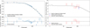 |
Fig. 9 Comparison of the surface density profile (left) and the velocity dispersion profile (right) of NGC 6749 with the best-fitting N-body model from the grid of models from Baumgardt & Hilker (2018). The model and observations agree well. |
4.3 Comparison with simulations
In order to derive the physical parameters of NGC 6749 from the new velocity dispersion profile, we searched the grid of N-body simulations that produced the best match of the surface density and velocity dispersion profile of NGC 6749 from Baumgardt & Hilker (2018). In order to compare with the N-body simulations, we summed the observed radial and tangential velocity dispersions at each radius, which appeared to be justified because the velocity dispersion is close to isotropic over most of the radial range that we measured. We scaled all N-body simulations in radius to match the observed half-light radius of NGC 6749 and then interpolated in the grid of simulations to find the best-fitting N-body model. We then derived the physical parameters of NGC 6749 from the N-body simulations as described in Baumgardt & Hilker (2018). Fig. 9 shows the result of our fitting process. We obtained a good fit to the velocity dispersion and surface density of NGC 6749, and our proper motion velocity dispersion profile agrees well with the radial velocity dispersion profile for an assumed cluster distance of 7.6 kpc. We find a total cluster mass of MC = (5.53 ± 0.28) ∙ 105 M⊙, a projected central dispersion of σ0 = 8.0 ± 0.64 km s−1, an Μ/L ratio of M/L = 3.65 ± 0.27 M⊙/L⊙, and a half-mass radius of rh = 7.1 pc. This places NGC 6749 among the 10% most massive GCs in the MW.
5 Conclusions
As a part of the MGCS treasury program (Massari et al. 2025), we presented new HST observations of NGC 6749 that we used to develop new publicly available Python-based tools for the photometric-based membership determination and kinematic analysis of GCs (and GC-like objects).
By combining our MGCS HST observations (Massari et al. 2025) with Gaia DR3 using the software GAIAHUB, we determined unprecedentedly precise PMs for this GC. In particular, we were able to decrease the PM error by up to one order of magnitude at the faint end (G > 18.5), and for the first time, we determine PMs for stars that only had Gaia positions measured so far.
We analyzed the resulting VPD of NGC 6749 using GMM. This method comprises an inference-based approach that uses MCMC simulations to find the posterior distribution of the model parameters. Our model has the flexibility of managing an arbitrary number of Gaussian components and can fix and/or link any parameter to another. A natural product of this procedure is the probability of each star to belong to NGC 6749. We compared this kinematic membership with that stemming from a photometric approach that combines a statistical CMD subtraction, featured with an adaptive Voronoi-based grid generation, with correction for differential reddening. This iterative approach improved the membership probability and differential reddening correction at each iteration. The comparison between the two methods is remarkably good, with the photometric algorithm ensuring an appropriate CMD decontamination even for stars that are too faint to have PM information.
Our kinematic analysis was first validated with a mock catalog and then with existing kinematic measurements, thus verifying the efficacy of our method in separating cluster and field components even in a relatively highly contaminated case. The mean motion of NGC 6749 of μα,δ = (−2.82, −5.99) ± 0.008 mas yr−1 was determined with a precision better than Gaia. Given the large number of stars with a precise PM measurement, we were able to investigate the kinematic profiles of NGC 6749 for the first time. By using a golden sample of PMs that combined the best measurements from ours and Gaia catalogs, we built the profiles of μrad,tan, σrad,tan, and the anisotropy (σtan/σrad). The general kinematic picture of GCs drawn by HST (Libralato et al. 2022) agrees overall. Finally, the comparison of our observed kinematic profile with N-body simulations revealed that NGC 6749 belongs to the 10% most massive GC in the Galaxy, with a total mass of M = (5.53 ± 0.28) ∙ 105 M⊙.
Data availability
All the tools presented here are available at the GitHub repository https://github.com/LR-inaf/MGCS_pytools.git or at the PyPi repository https://pypi.org/project/MGCS-pytools/.
Acknowledgements
D.M., S.C., E.P. and A.M. acknowledge financial support from PRIN-MIUR-22: CHRONOS: adjusting the clock(s) to unveil the CHRONO-chemo-dynamical Structure of the Galaxy” (PI:S. Cassisi). A.M. and M.B. acknowledge support from the project “LEGO - Reconstructing the building blocks of the Galaxy by chemical tagging” (PI: A. Mucciarelli), granted by the Italian MUR through contract PRIN 2022LLP8TK_001. M.M. acknowledges support from the Agencia Estatal de Investigación del Ministerio de Ciencia e Innovación (MCIN/AEI) under the grant “RR Lyrae stars, a lighthouse to distant galaxies and early galaxy evolution” and the European Regional Development Fun (ERDF) with reference PID2021-127042OB-I00. Co-funded by the European Union (ERC-2022-AdG, “StarDance: the non-canonical evolution of stars in clusters”, Grant Agreement 101093572, PI: E. Pancino). Views and opinions expressed are however those of the author(s) only and do not necessarily reflect those of the European Union or the European Research Council. Neither the European Union nor the granting authority can be held responsible for them. This paper is supported by the Italian Research Center on High Performance Computing Big Data and Quantum Computing (ICSC), project funded by European Union - NextGenerationEU - and National Recovery and Resilience Plan (NRRP) - Mission 4 Component 2 within the activities of Spoke 3 (Astrophysics and Cosmos Observations). This work is part of the project Cosmic-Lab at the Physics and Astronomy Department “A. Righi” of the Bologna University (http://www.cosmic-lab.eu/Cosmic-Lab/Home.html). Based on observations with the NASA/ESA HST, obtained at the Space Telescope Science Institute, which is operated by AURA, Inc., under NASA contract NAS 5-26555. Support for Program number GO-17435 was provided through grants from STScI under NASA contract NAS5-26555. This research made use of emcee (Foreman-Mackey et al. 2013). This work has made use of data from the European Space Agency (ESA) mission Gaia (https://www.cosmos.esa.int/gaia), processed by the Gaia Data Processing and Analysis Consortium (DPAC, https://www.cosmos.esa.int/web/gaia/dpac/consortium). Funding for the DPAC has been provided by national institutions, in particular the institutions participating in the Gaia Multilateral Agreement. ED acknowledges financial support from the INAF Data Analysis Research Grant (PI E. Dalessandro) of the “Bando Astrofisica Fondamentale 2024”.
References
- Anderson, J. 2022a, One-Pass HST Photometry with hst1pass, Instrument Science Report ACS 2022-02 [Google Scholar]
- Anderson, J. 2022b, One-Pass HST Photometry with hst1pass, Instrument Science Report WFC3 2022-5, 55 [Google Scholar]
- Anderson, J., & Ryon, J. E. 2018, Improving the Pixel-Based CTE-correction Model for ACS/WFC, Instrument Science Report ACS 2018-04, 37 [Google Scholar]
- Baumgardt, H., & Hilker, M. 2018, MNRAS, 478, 1520 [Google Scholar]
- Baumgardt, H., & Vasiliev, E. 2021, MNRAS, 505, 5957 [NASA ADS] [CrossRef] [Google Scholar]
- Bellini, A., Anderson, J., van der Marel, R. P., et al. 2014, ApJ, 797, 115 [Google Scholar]
- Bellini, A., Anderson, J., Bedin, L. R., et al. 2017, ApJ, 842, 6 [NASA ADS] [CrossRef] [Google Scholar]
- Bennet, P., Patel, E., Sohn, S. T., et al. 2024, ApJ, 971, 98 [Google Scholar]
- Bianchini, P., van der Marel, R. P., del Pino, A., et al. 2018, MNRAS, 481, 2125 [Google Scholar]
- Bonatto, C., & Bica, E. 2007, MNRAS, 377, 1301 [NASA ADS] [CrossRef] [Google Scholar]
- Cabrera-Ziri, I., Niederhofer, F., Bastian, N., et al. 2016, MNRAS, 459, 4218 [NASA ADS] [CrossRef] [Google Scholar]
- Callingham, T. M., Cautun, M., Deason, A. J., et al. 2022, MNRAS, 513, 4107 [NASA ADS] [CrossRef] [Google Scholar]
- Ceccarelli, E., Mucciarelli, A., Massari, D., Bellazzini, M., & Matsuno, T. 2024, A&A, 691, A226 [NASA ADS] [CrossRef] [EDP Sciences] [Google Scholar]
- Chen, Y., & Gnedin, O. Y. 2024, arXiv e-prints [arXiv:2401.17420] [Google Scholar]
- Dalessandro, E., Cadelano, M., Della Croce, A., et al. 2024, A&A, 691, A94 [NASA ADS] [CrossRef] [EDP Sciences] [Google Scholar]
- Dalessandro, E., Ferraro, F. R., Bastian, N., et al. 2019, A&A, 621, A45 [NASA ADS] [CrossRef] [EDP Sciences] [Google Scholar]
- De Angeli, F., Piotto, G., Cassisi, S., et al. 2005, AJ, 130, 116 [NASA ADS] [CrossRef] [Google Scholar]
- del Pino, A., Libralato, M., van der Marel, R. P., et al. 2022, ApJ, 933, 76 [NASA ADS] [CrossRef] [Google Scholar]
- Dotter, A., Sarajedini, A., Anderson, J., et al. 2010, ApJ, 708, 698 [Google Scholar]
- Foreman-Mackey, D., Hogg, D. W., Lang, D., & Goodman, J. 2013, PASP, 125, 306 [Google Scholar]
- Gaia Collaboration (Vallenari, A., et al.) 2023, A&A, 674, A1 [NASA ADS] [CrossRef] [EDP Sciences] [Google Scholar]
- Häberle, M., Neumayer, N., Seth, A., et al. 2024, Nature, 631, 285 [CrossRef] [Google Scholar]
- Harris, W. E. 1996, AJ, 112, 1487 [Google Scholar]
- Horta, D., Schiavon, R. P., Mackereth, J. T., et al. 2020, MNRAS, 493, 3363 [NASA ADS] [CrossRef] [Google Scholar]
- Knoetig, M. L. 2014, ApJ, 790, 106 [NASA ADS] [CrossRef] [Google Scholar]
- Leaman, R., VandenBerg, D. A., & Mendel, J. T. 2013, MNRAS, 436, 122 [Google Scholar]
- Libralato, M., Bellini, A., van der Marel, R. P., et al. 2018, ApJ, 861, 99 [CrossRef] [Google Scholar]
- Libralato, M., Bellini, A., Vesperini, E., et al. 2022, ApJ, 934, 150 [NASA ADS] [CrossRef] [Google Scholar]
- Libralato, M., Bedin, L. R., Griggio, M., et al. 2024, A&A, 692, A96 [NASA ADS] [CrossRef] [EDP Sciences] [Google Scholar]
- Marín-Franch, A., Aparicio, A., Piotto, G., et al. 2009, ApJ, 694, 1498 [Google Scholar]
- Massari, D., Breddels, M. A., Helmi, A., et al. 2018, Nat. Astron., 2, 156 [Google Scholar]
- Massari, D., Koppelman, H. H., & Helmi, A. 2019, A&A, 630, L4 [NASA ADS] [CrossRef] [EDP Sciences] [Google Scholar]
- Massari, D., Helmi, A., Mucciarelli, A., et al. 2020, A&A, 633, A36 [NASA ADS] [CrossRef] [EDP Sciences] [Google Scholar]
- Massari, D., Aguado-Agelet, F., Monelli, M., et al. 2023, A&A, 680, A20 [NASA ADS] [CrossRef] [EDP Sciences] [Google Scholar]
- Massari, D., Bellazzini, M., Libralato, M., et al. 2025, The Hubble Missing Globular Cluster Survey. I. Survey overview and the first precise age estimate for ESO452-11 and 2MASS-GC01 [Google Scholar]
- Mighell, K. J., Rich, R. M., Shara, M., & Fall, S. M. 1996, AJ, 111, 2314 [Google Scholar]
- Milone, A. P., Piotto, G., Bedin, L. R., et al. 2012, A&A, 540, A16 [NASA ADS] [CrossRef] [EDP Sciences] [Google Scholar]
- Milone, A. P., Marino, A. F., Di Criscienzo, M., et al. 2018, MNRAS, 477, 2640 [Google Scholar]
- Monty, S., Belokurov, V., Sanders, J. L., et al. 2024, MNRAS, 533, 2420 [NASA ADS] [CrossRef] [Google Scholar]
- Nardiello, D., Libralato, M., Piotto, G., et al. 2018, MNRAS, 481, 3382 [NASA ADS] [CrossRef] [Google Scholar]
- Piotto, G., Milone, A. P., Bedin, L. R., et al. 2015, AJ, 149, 91 [Google Scholar]
- Recio-Blanco, A. 2018, A&A, 620, A194 [NASA ADS] [CrossRef] [EDP Sciences] [Google Scholar]
- Sarajedini, A., Bedin, L. R., Chaboyer, B., et al. 2007, AJ, 133, 1658 [Google Scholar]
- Searle, L., & Zinn, R. 1978, ApJ, 225, 357 [Google Scholar]
- Sollima, A., Baumgardt, H., & Hilker, M. 2019, MNRAS, 485, 1460 [Google Scholar]
- Vasiliev, E., & Baumgardt, H. 2021, MNRAS, 505, 5978 [NASA ADS] [CrossRef] [Google Scholar]
- Watkins, L. L., van der Marel, R. P., Libralato, M., et al. 2022, ApJ, 936, 154 [CrossRef] [Google Scholar]
We made use of _flc exposures, i.e., dark- and bias-corrected, flat-fielded, nonresampled images that were pipeline-corrected for the charge-transfer-efficiency defects (Anderson & Ryon 2018).
The code and its ancillary files can be found here: https://www.stsci.edu/~jayander/HST1PASS/
Can be found in https://www.stsci.edu/~jayander/../STDGDCs/
Skew terms represent the deviation from orthogonality and the relative scale difference between the two axes.
For completeness, we also tested the membership option (–members flag) and found a slightly worse result because the contaminating field component and the cluster stars overlap significantly, which makes the membership selection challenging.
For a magnitude below G ≃ 18.5, the raw GH PMs are still better than those of Gaia. In particular, the median error value for GH is δμ = 0.04 mas/yr compared to δμ = 0.22 mas/yr for Gaia, but after the calibration described in Appendix A, the error increase due to the square-root summation of the initial error with the uncertainty on the correction.
We focused on well-measured sources identified photometrically by means of a mix of percentile-based selections on the quality of the ePSF fit, magnitude rms, and stellarity index, number of images used in the flux measurement, impact of the neighbor flux, and local sky (see, e.g., Libralato et al. 2022; Massari et al. 2025, and Libralato et al., in prep.).
The value of ten stars worked for this cluster, but this number has to be evaluated for each case, depending on the number of available stars.
Baumgardt H., private communication.
Quoted in people.smp.uq.edu.au/HolgerBaumgardt/globular/orbits
Appendix A Systematic correction
We extensively checked for systematics introduced by GAIAHUB and we found a non-linear correlation between μδ and the position of stars in the field of view, in particular with the δ coordinate (see Fig. A.1a). Firstly, we cross-checked this relation with the pure Gaia DR3 PM and we did not found any significant relation, reinforcing the idea of having introduced a systematic using GAIAHUB. We then choose to use Gaia as reference to compensate for this dependence. We corrected the GH PM of each star by subtracting the difference between itself and the median value of the Gaia PMs of the 25 neighbors stars. With this approach we were able to remove the systematic, obtaining an uncorrelated μδ against δ (see Fig. A.1b).
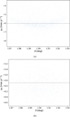 |
Fig. A.1 GH PMs δ component against the sky δ coordinate. (a) The uncorrected PMs and (b) after the correction. The gray dashed line shows the median value of the distribution, used as visual reference. |
All Tables
All Figures
|
Fig. 1 Colored image of NGC 6749 using the new HST (ACS/WFC) observations. The white cross shows the center of the cluster (according to Baumgardt & Vasiliev 2021), and the radius of the white circle is equal to the half-light radius. |
| In the text | |
|
Fig. 2 Comparison between the Gaia and GH PMs. The top panels show the VPDs of the PMs, and the two bottom panels show the PM errors along α cos δ and δ as a function of Gaia G magnitude. The black dots refer to the Gaia PMs, and the blue and red dots show stars in our catalog with and without a corresponding PM in the Gaia catalog, respectively. |
| In the text | |
|
Fig. 3 VPD (left panel) and CMDs (middle and right panels) of NGC 6749 using the new HST data of the MGCS survey. The red circle with the radius of 1 mas yr−1 in the VPD was used to select likely cluster stars (those included within the circle). In the central CMD, the gray dots represent all stars in our HST photometric catalog, and the black and red dots are foreground and cluster stars, respectively, for which we have a PM measurements. The horizontal dashed line corresponds to the Gaia limiting magnitude. Finally, the right panel shows the location of cluster member stars in the CMD. |
| In the text | |
|
Fig. 4 Distribution of the NGC 6749 GH PMs. The central scatter plot shows the 2D VPD, where the points are color-coded by the membership probability obtained from the MCMC chains (color bar). The top and right histograms show the normalized marginal distributions of the PMs, together with the posterior distributions of the GMM components, the target in red, the field in blue, and their sum in gray. |
| In the text | |
|
Fig. 5 Result of the statistical decontamination. (Top left panel) Contaminated target CMD. (Top right panel) Parallel field CMD. (Bottom left panel) Target CMD color-coded for the membership probability. (Bottom right panel) Membership probability distribution. The target CMDs were corrected for the differential reddening. |
| In the text | |
|
Fig. 6 Color-coded CMDs according to the membership probability. (Left) Membership calculated from the PMs. (Right) Membership obtained with the statistical approach. |
| In the text | |
|
Fig. 7 Comparison of the mean velocity (left) and velocity dispersion (right) components for GH (orange), and GaiaDR3-VB21 (blue). The error bars are the 16th and 84th of the posterior parameter distribution. The current line-of-sight velocity dispersion (black) is shown as reference. |
| In the text | |
|
Fig. 8 Radial profiles of the mean velocity (μrad,tan), velocity dispersion (σrad,tan), and anisotropy (calculated as |
| In the text | |
|
Fig. 9 Comparison of the surface density profile (left) and the velocity dispersion profile (right) of NGC 6749 with the best-fitting N-body model from the grid of models from Baumgardt & Hilker (2018). The model and observations agree well. |
| In the text | |
|
Fig. A.1 GH PMs δ component against the sky δ coordinate. (a) The uncorrected PMs and (b) after the correction. The gray dashed line shows the median value of the distribution, used as visual reference. |
| In the text | |
Current usage metrics show cumulative count of Article Views (full-text article views including HTML views, PDF and ePub downloads, according to the available data) and Abstracts Views on Vision4Press platform.
Data correspond to usage on the plateform after 2015. The current usage metrics is available 48-96 hours after online publication and is updated daily on week days.
Initial download of the metrics may take a while.