© The Authors 2026

1. Introduction

By combining magnetohydrodynamic (MHD) wave theory with observations, coronal seismology provides inversion schemes to indirectly infer some physical parameters, such as the coronal magnetic field (see, e.g., Nakariakov & Kolotkov 2020, for a recent review). As the only MHD wave mode that can disturb the axis of magnetic structures, kink waves can be used to diagnose the coronal magnetic field based on their measured frequencies regardless of standing or propagating waves (e.g., Nakariakov & Ofman 2001; Yang et al. 2020a,b, 2024). However, current seismology schemes are still based on the theoretical framework of kink modes in canonical magnetic cylinders (e.g., Zajtsev & Stepanov 1975; Edwin & Roberts 1983). Gravity and curvature of coronal loops are essential, but have not yet been taken into account simultaneously in the context of coronal seismology.

As a typical magnetic structure in the solar corona, curved loops are known to be typical waveguides for kink waves (e.g., Reale 2014; Nakariakov & Kolotkov 2020). The influence of loop curvature on kink modes was initially explored in two-dimensional (2D) models (e.g., Smith et al. 1997; Brady & Arber 2005; Selwa et al. 2005; Verwichte et al. 2006a,b,c). These studies were restricted to the examination of vertical polarizations, which can be excited, for example, by slow modes in short loops (Lopin & Nagorny 2024) or vortex shedding (Karampelas & Van Doorsselaere 2021). Although vertical polarizations have also been confirmed in observations (e.g., Wang & Solanki 2004; Wang et al. 2008), the other polarization, namely the more frequently observed horizontal kink polarization (e.g., Zhong et al. 2023), should also be examined. Analytically, Van Doorsselaere et al. (2004, 2009) found that the curvature in a toroidal loop model has little influence on kink eigenmodes under a force-free magnetic field. Numerically, the frequency difference between horizontally and vertically polarized kink oscillations has been found not to be observable in a semi-torus model (Terradas et al. 2006). Considering the Wentzel-Kramers-Brillouin (WKB) approximation, Magyar & Nakariakov (2020) showed that the analytical prediction can reasonably describe the kink frequency in their planar model. More recently, Guo et al. (2024) examined the oscillation and damping properties for both horizontal and vertical polarizations, comparing their results with previous studies of different kink polarizations (Ruderman 2009; Guo et al. 2020). However, these studies on kink oscillations in curved loop models do not consider the effect of gravitational stratification.

In long coronal loops whose lengths significantly exceed the gravitational scale height, gravitational stratification is expected to influence loop dynamics. Density stratification affects the displacements of fundamental kink modes in coronal loops (e.g., Erdélyi & Verth 2007). Andries et al. (2005b) analytically investigated the influence of longitudinal density stratification on the frequencies and damping rates of kink eigenmodes. Furthermore, based on deviations in the period ratio between the fundamental mode and the first overtone (i.e., P₁/P₂) from 2, the density stratification can be determined (Andries et al. 2005a; Van Doorsselaere et al. 2007). However, magnetic-stratification-induced loop expansion can increase P₁/P₂, and thus significantly affect the results of coronal seismology (Verth & Erdélyi 2008). Regarding the propagation of kink modes, the effect of gravitational stratification was analytically investigated by Spruit (1981), who introduced a global cutoff. Although Lopin et al. (2014) offered a different perspective of the cutoff for kink waves in a stratified atmosphere, recent numerical work by Pelouze et al. (2023) has helped to clarify the physical scenario. In recent numerical studies of kink oscillations in magnetic cylinders, gravity is routinely included in the contexts of both seismology (e.g., Gao et al. 2024, 2025) and coronal heating (e.g., Karampelas et al. 2019). However, none of these studies of kink waves in stratified loops have simultaneously incorporated the effects of loop curvature.

The combined effects of gravity and loop curvature on kink oscillations have not yet been investigated in the same model. In the current work, we examine kink eigenmodes in a curved coronal loop with the presence of gravity. This paper is organized as follows. Section 2 describes the equilibrium and the numerical setup. The simulation results are presented and discussed in Sects. 3 and 4, followed by a summary of the present work in Sect. 5.

2. Model description

We considered a potential magnetic field similar to that in Guo et al. (2024). In a Cartesian coordinate system (x, y, z), the initial magnetic field is given by

$$\begin{array}{cc}\hfill B_x(x,z)& =B_{0}cos\left({\displaystyle \frac{x}{{\mathrm{\Lambda }}_B}}\right)exp\left({\displaystyle -\frac{z}{{\mathrm{\Lambda }}_B}}\right),\hfill \\ \hfill B_z(x,z)& =-B_{0}sin\left({\displaystyle \frac{x}{{\mathrm{\Lambda }}_B}}\right)exp\left({\displaystyle -\frac{z}{{\mathrm{\Lambda }}_B}}\right),\hfill \end{array}$$(1)

where B₀ = 30 G, Λ_B = 2L_B/π with L_B = 145 Mm. We also defined a set of orthonormal basis vectors $({\widehat{\mathit{e}}}_{\mathrm{t}},{\widehat{\mathit{e}}}_{\mathrm{h}},{\widehat{\mathit{e}}}_{\mathrm{v}})$,

$$\begin{array}{cc}\hfill {\widehat{\mathit{e}}}_{\mathrm{t}}& =cos(x/{\mathrm{\Lambda }}_B)\widehat{x}-sin(x/{\mathrm{\Lambda }}_B)\widehat{z},\hfill \\ \hfill {\widehat{\mathit{e}}}_{\mathrm{h}}& =\widehat{y},\hfill \\ \hfill {\widehat{\mathit{e}}}_{\mathrm{v}}& =sin(x/{\mathrm{\Lambda }}_B)\widehat{x}+cos(x/{\mathrm{\Lambda }}_B)\widehat{z}.\hfill \end{array}$$(2)

In the x − z plane, ${\widehat{\mathit{e}}}_{\mathrm{t}}$ (${\widehat{\mathit{e}}}_{\mathrm{v}}$) is locally parallel (perpendicular) to the magnetic field.

We then considered a vertically stratified atmosphere. The gravity is given by

$$\begin{array}{c}\hfill \mathit{g}(z)=-\frac{g_{\odot }{R}_{\odot }^2}{{(z+R_{\odot })}^2}\widehat{z},\end{array}$$(3)

where g_⊙ is the gravitational acceleration on the solar surface, and R_⊙ is the solar radius. The stratified background pressure and density are described by

$$\begin{array}{c}\hfill \frac{\mathrm{d}p(z)}{\mathrm{d}z}=-\frac{g_{\odot }{R}_{\odot }^2}{{(z+R_{\odot })}^2}\rho (z).\end{array}$$(4)

Note that the background temperature is constant. Combined with the ideal gas law, we can readily obtain the density and pressure of the background:

$$\begin{array}{cc}\hfill {\rho }_{\mathrm{e}}(z)& ={\rho }_{\mathrm{e}0}exp(\frac{-g_{\odot }{R}_{\odot }}{A_0{T}_{\mathrm{e}}}+\frac{g_{\odot }{R}_{\odot }^2}{A_0{T}_{\mathrm{e}}}\frac{1}{z+R_{\odot }}),\hfill \end{array}$$(5)

$$\begin{array}{cc}\hfill p_{\mathrm{e}}(z)& =A_0{T}_{\mathrm{e}}{\rho }_{\mathrm{e}}(z),\hfill \end{array}$$(6)

where A₀ = 2k_B/m_H, T_e = 2 MK, ρ_e0 = 4.18 × 10⁻¹⁶ g cm⁻³.

The density-enhanced loop was then constructed. The internal loop density and pressure profiles at a given height, z, are

$$\begin{array}{cc}\hfill {\rho }_{\mathrm{i}}(z)& =2{\rho }_{\mathrm{e}0}exp(\frac{-g_{\odot }{R}_{\odot }}{A_0{T}_{\mathrm{i}}}+\frac{g_{\odot }{R}_{\odot }^2}{A_0{T}_{\mathrm{i}}}\frac{1}{z+R_{\odot }}),\hfill \end{array}$$(7)

$$\begin{array}{cc}\hfill p_{\mathrm{i}}(z)& =A_0{T}_{\mathrm{i}}{\rho }_{\mathrm{i}}(z),\hfill \end{array}$$(8)

where T_i = 1 MK. This ensures a density ratio of 2 between the internal loop region and the external corona at z = 0. The density and pressure distributions are given by

$$\begin{array}{cc}\hfill \rho (\overline{r})& {\displaystyle ={\rho }_{\mathrm{e}}(z)+\frac{{\rho }_{\mathrm{i}}(z)-{\rho }_{\mathrm{e}}(z)}{2}\{1-tanh\left[\left({\displaystyle \frac{\overline{r}}{R}-1}\right)b\right]\},}\hfill \end{array}$$(9)

$$\begin{array}{cc}\hfill p(\overline{r})& {\displaystyle =p_{\mathrm{e}}(z)+\frac{p_{\mathrm{i}}(z)-p_{\mathrm{e}}(z)}{2}\{1-tanh\left[\left({\displaystyle \frac{\overline{r}}{R}-1}\right)b\right]\},}\hfill \end{array}$$(10)

where

$$\begin{array}{c}\hfill \overline{r}=\sqrt{{\left({\displaystyle \frac{\psi -{\psi }_0}{\mathrm{\Delta }\psi }}\right)}^2+{\left({\displaystyle \frac{y}{\mathrm{\Delta }y}}\right)}^2},\end{array}$$(11)

with

$$\begin{array}{c}\hfill \psi =B_0{\mathrm{\Lambda }}_{B}cos\left({\displaystyle \frac{x}{{\mathrm{\Lambda }}_B}}\right)exp\left({\displaystyle -\frac{z}{{\mathrm{\Lambda }}_B}}\right),\end{array}$$(12)

and ψ₀ = ψ(x = 100 Mm, z = 0), Δψ = B₀Λ_B, Δy = 2Λ_B. Here, R = cos(100/Λ_B) − cos(101/Λ_B) prescribes the x extent of the loop at its footpoints. The parameter b = 10 determines the width of the boundary layer. Note that the density enhanced loop is in a low-β environment with a maximum plasma β of 0.016. The 3D view of the initial state is shown in Fig. 1a.

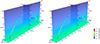Fig. 1. 3D rendering of the density-enhanced loop. Left: Initial state before relaxation. Right: Relaxed state.

Before proceeding, we need to specify our numerical setup. Regarding the bottom boundary at z = 0, all the components of the velocity are set to vanish, while all the components of the magnetic field follow the zero gradient condition. The density and pressure were fixed at their initial values. Outflow boundary conditions were applied to all the other side boundaries. To ensure the stability of the computation, we also considered a velocity absorption layer (see also Pelouze et al. 2023; Guo et al. 2023; Gao et al. 2024). The velocity was modified by

$$\begin{array}{c}\hfill v^{\prime }(x,y,z;t)=\alpha (t)\gamma (z)v(x,y,z;t),\end{array}$$(13)

where

$$\begin{array}{c}\hfill \alpha (t)=\{\begin{array}{cc}{\displaystyle 0.998+0.002\frac{t}{t_c},}\hfill & 0<t\le t_{\mathrm{c}},\hfill \\ 1,\hfill & t>t_{\mathrm{c}},\hfill \end{array}\end{array}$$(14)

and

$$\begin{array}{c}\hfill \gamma (z)=0.5\{1-tanh\left[0.3\left(\frac{z-90}{l_0}\right)\right]\},\end{array}$$(15)

with t_c = 2000 s and l₀ = 1 Mm being the unit of length. We then solved the set of ideal 3D MHD equations with the PLUTO code (Mignone et al. 2007). As in Guo et al. (2024), a similar magnetic field splitting method was used. We chose the piecewise parabolic scheme for spatial reconstruction, the HLLD Riemann solver to calculate the numerical fluxes, and the second-order Runge–Kutta method for time marching. The computational domain is [ − 120, 120]×[−15, 15]×[0, 100] Mm. We adopted a set of uniform grid with 600 × 120 × 400 cells.

Note that relaxation is necessary, as it is not a magnetostatic balance system so far. The system reaches equilibrium after a relaxation period of 2000 s, and the relaxed state is shown in Fig. 1b. In the following, we consider this relaxed state to be t = 0. The maximum residual velocity in the system is less than 2 km/s. Since the characteristic evolution timescale of the system, |δρ/[∇⋅(ρv)]|, is much longer than the period of the wave of interest, the system can thus be regarded as a stable state.

Then we specified the initial perturbations. We distinguished two different polarizations; namely, horizontal and vertical. As is discussed in Guo et al. (2024), the density distribution across the loop cross section is no longer axisymmetric due to gravity-induced stratification. Since the density remains nearly constant in the horizontal direction at a given height, horizontally polarized modes experience little influence from stratification. In contrast, vertically polarized kink modes are expected to be more strongly affected by gravitational stratification.

In the following, we first focus on vertical polarization. Similar to the initial conditions in Guo et al. (2024), we introduced an initial velocity perturbation of the form

$$\begin{array}{c}\hfill {\displaystyle \mathit{v}(x,y,z;t=0)=\frac{v_{0}sin\theta }{2}\{1-tanh\left[\left({\displaystyle \frac{\overline{r}}{R}-1}\right)b\right]\}{\widehat{\mathit{e}}}_{\mathrm{v}},}\end{array}$$(16)

where v₀ = 20 km/s is the amplitude of the velocity perturbation, $sin\theta =\frac{z}{\sqrt{x^2+z^2}}$ with θ being the angle along the loop from the bottom. It ensures maximum velocity perturbation at loop apex and zero velocity at loop footpoints. For reference, we also considered a horizontal velocity perturbation in the y direction,

$$\begin{array}{c}\hfill {\displaystyle \mathit{v}(x,y,z;t=0)=\frac{v_{0}sin\theta }{2}\{1-tanh\left[\left({\displaystyle \frac{\overline{r}}{R}-1}\right)b\right]\}{\widehat{\mathit{e}}}_{\mathrm{h}}.}\end{array}$$(17)

In addition, we also considered another set of initial velocity conditions to excite the first overtones. The velocity perturbation in the vertical direction is given by

$$\begin{array}{c}\hfill \mathit{v}(x,y,z;t=0)=v_{0}sin\theta cos\theta \{1-tanh\left[\left({\displaystyle \frac{\overline{r}}{R}-1}\right)b\right]\}{\widehat{\mathit{e}}}_{\mathrm{v}},\end{array}$$(18)

and the horizontal velocity perturbation is given by

$$\begin{array}{c}\hfill \mathit{v}(x,y,z;t=0)=v_{0}sin\theta cos\theta \{1-tanh\left[\left({\displaystyle \frac{\overline{r}}{R}-1}\right)b\right]\}{\widehat{\mathit{e}}}_{\mathrm{h}}.\end{array}$$(19)

3. Results

We first examined the frequency of the vertical polarization. To better compare the results with analytical predictions, we tracked the Lagrangian displacement of a fluid parcel. This was implemented by assigning the passive tracer in the code. As such, we could follow the displacement of a fluid parcel within the loop region. The solid lines in Fig. 2 show the temporal evolution of the Lagrangian velocity of the specified fluid parcels. Different fluid parcels in the loop were sampled, as is distinguished by different colors. One fluid parcel was initially located at the loop apex ([x, y, z]=[0, 0, 70] Mm) at t = 0; the other two fluid parcels were initially located at one quarter position of the loop ([x, y, z]=[59.4, 0, 49.4] Mm) and the opposite quarter of the loop ([x, y, z]=[−59.4, 0, 49.4] Mm). Following a procedure similar to that in Guo et al. (2020, 2024), we estimated the oscillation period as twice the average time interval between two adjacent extrema of the oscillating profile. For the loop apex (black solid curve), this procedure yields a period of $P_{\mathrm{v}}^{\mathrm{fun}}=221.6$ s, while the oscillation period at the other two quarters of the loop is 226 s. Neglecting the small measurement errors at different locations, we find that the periods are similar. We also find that these oscillation profiles are in phase, and that the two quarters of the loop exhibit the same oscillation behavior. This clearly indicates that the excited oscillation in the current loop corresponds to the fundamental mode. To be consistent with observations, we used the period at the loop apex to represent the oscillation period in the loop hereafter.

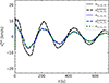Fig. 2. Temporal evolution of vv for the vertically polarized fundamental kink oscillations. The black, blue, and green lines represent vv of fluid parcels initially located at the loop apex ([x0, y0, z0]=[0, 0, 70] Mm), at one quarter of the loop ([x1, y1, z1]=[59.4, 0, 49.4] Mm), and at the opposite quarter of the loop ([x2, y2, z2]=[−59.4, 0, 49.4] Mm), respectively. The dashed black and blue line designate vv measured at the fixed position [x0, y0, z0] and [x1, y1, z1].

Under some assumptions in a straight magnetic cylinder, such as the thin-tube-thin-boundary (TTTB) approximation, the period can be predicted through modal analysis (e.g., Edwin & Roberts 1983; Goossens et al. 1992). When the Alfvén frequency varies along the loop axis, the oscillation frequency can be estimated using the WKB approximation. For loops with an axisymmetric density profile across the loop, the WKB approximation can describe the oscillation frequency quite well (Guo et al. 2024). In the current model, applying the WKB approximation yields a predicted period of

$$\begin{array}{c}\hfill {\displaystyle P_{\mathrm{WKB}}=2{\displaystyle {\int }_0^L}\frac{\mathrm{d}s}{c_{\mathrm{k}}(s)}=2{\displaystyle {\int }_0^L}\sqrt{\frac{{\rho }_{\mathrm{i}}(s)+{\rho }_{\mathrm{e}}(s)}{2{\rho }_{\mathrm{i}}(s)}}\frac{\mathrm{d}s}{v_{\mathrm{Ai}}\left(s\right)},}\end{array}$$(20)

with

$$\begin{array}{c}\hfill {\displaystyle v_{\mathrm{Ai}}\left(s\right)=\frac{B\left(s\right)}{\sqrt{{\mu }_0{\rho }_{\mathrm{i}}\left(s\right)}},}\end{array}$$(21)

where c_k is the kink speed, v_Ai is the internal Alfvén speed along the loop axis, L represents the loop length, s is the distance from a footpoint along the loop axis and can be expressed as a function of z, and B(s) is the magnetic field strength along s. According to this formula, we thus obtained a period of P_WKB = 188.3 s. Therefore, the oscillation period, P_v, deviates from this theoretical estimation (P_WKB) by approximately 18%.

In general, the Lagrangian velocity is expected to be different from the Eulerian velocity measured at a fixed position. However, in the current case, Fig. 2 shows that the Lagrangian velocity closely matches the velocity measured at the fixed positions (filled black circles in Fig. 2). This agreement can be understood by calculating the Lagrangian displacement from the perturbation amplitude and oscillation period. The resulting displacement is still smaller than the cross-sectional radius at the loop apex, confirming that the traced fluid parcel remains within the internal loop region with uniform velocity. In the following analysis, we focus on the Lagrangian velocity only.

Figure 3 shows horizontal oscillation profiles similar to those in Fig. 2. We can also compute the oscillation period from the different positions of the loop. At the apex (one quarter) of the loop, the period is measured as $P_{\mathrm{h}}^{\mathrm{fun}}=174.8$ s (178 s). The similar periods, as well as the in-phase property of different positions, again indicates that the excited horizontal oscillation in the current loop is an axial fundamental mode. We used the period at the loop apex to represent the oscillation period. Therefore, the oscillation period of the horizontal polarization deviates from P_WKB by only 7%.

Fig. 3. Similar to Fig. 2 but for the horizontal polarized fundamental kink oscillations.

We also examined the oscillation profiles of the first overtones. As for the fundamental modes, we considered both vertical and horizontal polarizations of the first overtones. Oscillation profiles at the loop apex, as well as at one quarter and the opposite quarter of the loop are presented in Figs. 4 and 5. As was expected for the first overtones, the oscillation at one quarter of the loop is in antiphase with that at the opposite quarter. The velocity at the loop apex is nearly zero, indicating that this location corresponds to a wave node. Before proceeding, we estimated the predicted period of the first overtones, which is half that of the fundamental modes; namely, 94.15 s. To determine the oscillation periods from the numerical results, the same procedure described in Fig. 2 was applied to the oscillation profiles here. We find that the oscillation period for the vertically polarized mode is $P_{\mathrm{v}}^{1\mathrm{st}}=95.4$ s, while that for the horizontally polarized mode is $P_{\mathrm{h}}^{1\mathrm{st}}=90.3$ s. Both values closely match the predicted period, with a maximum deviation of about 4%.

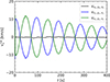Fig. 4. Temporal evolution of vv for the vertically polarized first overtones of kink oscillations. The black, blue, and green lines represent vv of fluid parcels initially located at the loop apex ([x0, y0, z0]=[0, 0, 70] Mm), at one quarter of the loop ([x1, y1, z1]=[59.4, 0, 49.4] Mm), and at the opposite quarter of the loop ([x2, y2, z2]=[−59.4, 0, 49.4] Mm), respectively.

The damping of the oscillation profiles can also be observed. It is widely accepted that resonant absorption is the dominant damping mechanism of kink oscillations (e.g., Goossens et al. 2002; Guo et al. 2024). However, resolving the resonant process within the boundary layer surrounding the loop requires a higher numerical resolution. Therefore, the damping process presented here may not be reliable. Nevertheless, in the present work, we mainly focus on the periods of different polarizations and harmonics, which are not significantly influenced by numerical resolutions.

In addition, we note that the oscillation profiles in Figs. 3 and 5 are not as sinusoidal as those in the other figures, showing some reverse steepening. This may result from the excitation of higher harmonics of the kink oscillations. However, a detailed examination is beyond the scope of the current work.

Fig. 5. Similar to Fig. 4 but for the horizontal first overtones of kink oscillations.

We further examined the distribution of the local Alfvén frequency to gain an insight into the oscillation period. Having the Alfvén speed distribution at hand, we can calculate the local Alfvén frequency distribution, ω_A(x, z). For axial fundamental modes and the first overtones, we have

$$\begin{array}{c}\hfill {\omega }_{\mathrm{A}}^{\mathrm{fun}}(x,z)=\frac{\pi }{\mathcal{L}(x,z)}{v}_{\mathrm{A}}(x,z)\end{array}$$(22)

and

$$\begin{array}{c}\hfill {\omega }_{\mathrm{A}}^{1\mathrm{st}}(x,z)=\frac{2\pi }{\mathcal{L}(x,z)}{v}_{\mathrm{A}}(x,z),\end{array}$$(23)

where ℒ is the length of the field line anchored at bottom boundary, threading a given point (x, z). Figure 6 shows the local Alfvén frequency distribution on the surface y = 0. We also translated the periods of different kink polarizations to frequencies for both the fundamental modes and the first overtones. In Fig. 6a the local Alfvén frequency distribution for the fundamental modes is illustrated. The frequency of the vertically polarized kink mode matches the local Alfvén frequency near the loop apex, as shown by the dashed black line. This suggests that we can use the local Alfvén frequency near the apex to predict the real oscillation frequency of the vertically polarized fundamental modes. When we move downward along the loop, the local Alfvén frequency increases. Near one quarter of the loop, the local frequency becomes comparable to both the value calculated from the WKB approximation, P_WKB, and the measured period, $P_{\mathrm{h}}^{\mathrm{fun}}$, of the horizontally polarized fundamental mode (dash-dotted line). As was mentioned before, WKB theory can describe the frequency of horizontal modes quite well, as has previously been confirmed by Guo et al. (2024). Figure 6b shows the local Alfvén frequency distribution for the first overtones. We also overplot the frequencies of both the vertically and horizontally polarized first overtones. Since the periods of the two polarizations are similar and closely match the WKB prediction, the frequencies for both polarizations can also be described by local Alfvén frequency near one quarter of the loop.

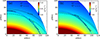Fig. 6. Map of the local Alfvén frequency on the y = 0 plane for (a) the fundamental modes and (b) the first overtones. The dashed (dash-dotted) lines represent contours of the frequencies corresponding to the vertical (horizontal) polarizations as labelled.

Furthermore, we can also see the dashed lines outside the loop region in Fig. 6. This leads to the wave tunneling effect and results in lateral leakage of the wave. This scenario has been discussed in Guo et al. (2024).

4. Discussion

4.1. Frequency deviations from WKB theory

To understand the deviation of the oscillation frequency from the WKB approximation, we should revisit the local Alfvén frequency. For kink modes, the oscillation frequency is determined by contributions from both the internal and external loop regions. As is shown in Fig. 6, the local Alfvén frequency decreases in the ${\widehat{e}}_{\mathrm{v}}$ direction (perpendicular to the magnetic field lines). Therefore, for the vertically polarized kink mode, regions with both higher and lower frequencies than that inside the loop become relevant. For vertically polarized fundamental modes, the damping of the oscillation (see Fig. 2) leads to an unequal contribution from the lower and upper loop regions. Given that the realistic oscillation is typically excited below the loop (e.g., Zimovets & Nakariakov 2015), leading to an initial upward motion, the upper loop region contributes more fractions. As a result, the measured oscillation frequency is lower than the WKB prediction. This is also consistent with previous results in Guo et al. (2024) when a uniform density loop is considered. In the current case, the deviation from the WKB approximation is larger. This is because gravitational stratification enhances the nonuniformity of the loop along its axis. Consequently, a steeper gradient develops in the local Alfvén frequency, which introduces greater uncertainty into the WKB approximation. For vertically polarized first overtones, the antiphase oscillation with respect to the apex decreases the above effect. Therefore, the deviations of the vertically polarized first overtones from the WKB approximation are quite small. In the horizontal case, the loop oscillates in the ${\widehat{e}}_{\mathrm{h}}$ direction of almost uniform local Alfvén frequencies, allowing the WKB approximation to predict the oscillation frequency with a smaller deviation.

The frequency of the vertically polarized fundamental mode matches the local Alfvén frequency near the loop apex. In principle, the frequency calculated from the WKB approximation should correspond to the local Alfvén frequency at some location in the loop region, as indicated by Eq. (20) and illustrated in Fig. 6. In the current model, as was discussed above, the measured frequency is lower than the WKB prediction, meaning that the oscillation frequency is shifted toward the loop apex. This is not coincidental, but rather a natural consequence of vertically polarized fundamental modes in the current model.

4.2. Implications for magnetic field measurements

The oscillation frequency serves as a key observable of kink modes in coronal loops. However, in seismology processes in stratified coronal loops, it should be emphasized that even when using a WKB approximation that incorporates axial nonuniformity (as in Sect. 3), the inversion process inherently retains a degree of uncertainty. In the case of horizontally polarized kink modes, this uncertainty remains acceptable, given that the observed oscillation frequency deviates from the WKB prediction by only about 5%. However, seismological application for vertically polarized kink modes requires greater caution when based solely on the WKB theory. In realistic gravitationally stratified loops, axial nonuniformity may lead to significant deviations in oscillation frequency. Nevertheless, we suggest that one should consider the local Alfvén frequency near the loop apex in potential seismology applications when the vertical kink polarization is involved to avoid large uncertainties.

The present results pave the way for spatially dependent inference of the coronal magnetic field strength. In coronal seismology, the magnetic field strength can be inferred from the kink speed, provided that the phase speed and density are known (e.g., Yang et al. 2020a,b, 2024). In the current scenario, as was discussed above, the measured periods of different fundamental polarizations reveal different local Alfvén frequencies. This provides a potential approach to probe the local magnetic field strength once the local density is determined. During the TRACE era, Wang et al. (2008) reported that different kink polarizations could coexist within the same coronal loop. However, unambiguous observation of kink polarizations has only become possible in recent years with multi-angle and high-resolution observations (e.g., Zhong et al. 2023). In addition, higher-temporal-resolution observations may further help to distinguish the different periods associated with different polarizations.

4.3. Scale height diagnostics

It is known that deviations of the period ratio, P₁/P₂ (i.e., P^fun/P^1st in the present context), from 2 can be used to diagnose the density scale height in a stratified atmosphere (e.g., Andries et al. 2005a; Van Doorsselaere et al. 2007). In our computations, in principle, the density scale height can be inferred, since we have obtained the period ratio, P^fun/P^1st, for different polarizations. Before proceeding, we first examined the initial density distribution along the loop axis. As is shown in Fig. 7, the density profile does not follow an exact exponential form, but still lies between two exponential functions; namely, exp(−z/60) and exp(−z/70). This indicates that the density distribution is close to exponential, with a scale height of between 60 Mm and 70 Mm. According to Andries et al. (2005a), the relationship between the period ratio, P^fun/P^1st, and the scale height, H, can be derived.

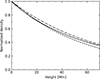Fig. 7. Initial density distribution along the loop axis. Dashed and dash-doted lines illustrate the function of exp(−z/60) and exp(−z/70), respectively.

From a different perspective, inspired by Dymova & Ruderman (2006), we considered solving the Sturm-Liouville problem:

$$\begin{array}{c}\hfill -\frac{{\mathrm{d}}^{2}u(s)}{\mathrm{d}{z}^2}=\frac{{\omega }^2}{c_{\mathrm{k}}^2(s)}u(s),u(s)=0\mathrm{at}s=0,L.\end{array}$$(24)

The procedure is to provide the nonuniform distribution of c_k(s) and then find the eigenvalues ω². In Andries et al. (2005a), a uniform magnetic field is assumed, so the kink speed c_k is

$$\begin{array}{c}\hfill c_{\mathrm{k}}(s)=\sqrt{\frac{2B_0^2}{{\mu }_0\rho (s)(1+{\rho }_{\mathrm{ie}})}},\end{array}$$(25)

where ρ_ie = 2 is the density ratio, and ρ(s) = ρ₀exp[−L/πHsin(πs/L)]. Then the period ratio P^fun/P^1st as a function of L/πH presented in Andries et al. (2005a) can be reproduced, as shown by the blue line in Fig. 8. However, the magnetic field inhomogeneity in our current model has not been included. We then take the variation of the magnetic field strength, namely B₀exp[−L/πΛ_Bsin(πs/L)], into account, and obtain another P^fun/P^1st versus L/πH curve, shown by the black line in Fig. 8. The difference between these two curves caused by the nonuniform magnetic field is evident, and the P^fun/P^1st even exceeds 2 in the black line when L/πH is small.

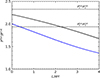Fig. 8. Period ratio, Pfun/P1st, as a function of the density stratification, L/πH. The solid curves were derived from Eq. (24). The dashed lines indicate the period ratio of $P_{\mathrm{h}}^{\mathrm{fun}}/P_{\mathrm{h}}^{1\mathrm{st}}$ and $P_{\mathrm{v}}^{\mathrm{fun}}/P_{\mathrm{v}}^{1\mathrm{st}}$ as labelled. See text for more details.

The period ratio exceeding 2 seems consistent with the results of Verth & Erdélyi (2008), who showed that loop expansion can increase the period ratio. In the current model, the loop radius is kept constant in the y direction but varies in the ${\widehat{e}}_v$ direction perpendicular to the magnetic field lines. As a result, only vertically polarized modes can feel the cross-sectional expansion from the footpoints to the loop apex. Consequently, the increase in radius in the ${\widehat{e}}_{\mathrm{v}}$ direction leads to a period ratio of the vertical polarizations greater than 2.

We then proceed to infer the density scale height. For the horizontally polarized case, we computed the period ratio between the fundamental mode and the first overtone as $P_{\mathrm{h}}^{\mathrm{fun}}/P_{\mathrm{h}}^{1\mathrm{st}}=1.94$. This period ratio corresponds to a scale height of approximately 40 Mm in our results, but exceeds 200 Mm according to the curve of Andries et al. (2005a), which is significantly larger than the actual scale height (60–70 Mm) of the model. This indicates that magnetic field inhomogeneity should be included in this inversion scheme. However, if we instead use the period ratio between the vertically polarized fundamental mode and the first overtone, namely $P_{\mathrm{v}}^{\mathrm{fun}}/P_{\mathrm{v}}^{1\mathrm{st}}=2.35$, the scale height cannot be derived because this value falls outside the range shown in Fig. 8.

5. Summary

We investigated the response of a gravitationally stratified coronal loop to different initial velocity perturbations. For the vertically polarized fundamental mode, the oscillation frequency deviates from the WKB approximation by approximately 18%. Nevertheless, the measured oscillation frequency aligns closely with the local Alfvén frequency near the loop apex. For the horizontally polarized fundamental mode, the oscillation frequency is reproduced well by the WKB theory, with a deviation of only 7%. Moreover, the frequency closely matches the local Alfvén frequency near one quarter of the loop. These results suggest that the local Alfvén frequency at the apex (quarter) of the loop can serve as a more accurate prediction of the frequency of vertically (horizontally) polarized fundamental kink oscillations in gravitationally stratified coronal loops. For the first overtones, the oscillation frequencies for both polarizations are close to the WKB approximation, and their frequencies are closely match the local Alfvén frequency close to one quarter of the loop.

Our findings open the possibility for spatially seismological inference of the coronal magnetic field. The measured periods of fundamental oscillations for different polarizations provide the corresponding local Alfvén frequencies and, consequently, could enable the probing of the magnetic field strength at multiple locations along the loop, provided that the local density can be obtained in observations.

In addition, the deviation of the period ratio between the fundamental mode and the first overtone, namely P^fun/P^1st, can be used to probe the density scale height in a stratified atmosphere. By comparison with the results of Andries et al. (2005a), we find that magnetic field inhomogeneity should be taken into account to obtain a more accurate estimate of the scale height.

Acknowledgments

This work is supported by the National Natural Science Foundation of China (12203030, 12373055, 12273019). M.G. also acknowledges the support from the QILU Young Scholars Program of Shandong University, the Taishan Scholars Program Special Fund (tsqn202408051) and the Shandong Provincial Natural Science Foundation for Excellent Young Scientists Program, Overseas (2025HWYQ-019).

References

All Figures

	Fig. 1. 3D rendering of the density-enhanced loop. Left: Initial state before relaxation. Right: Relaxed state.
In the text

Fig. 2. Temporal evolution of vv for the vertically polarized fundamental kink oscillations. The black, blue, and green lines represent vv of fluid parcels initially located at the loop apex ([x0, y0, z0]=[0, 0, 70] Mm), at one quarter of the loop ([x1, y1, z1]=[59.4, 0, 49.4] Mm), and at the opposite quarter of the loop ([x2, y2, z2]=[−59.4, 0, 49.4] Mm), respectively. The dashed black and blue line designate vv measured at the fixed position [x0, y0, z0] and [x1, y1, z1].

In the text

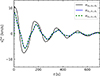	Fig. 3. Similar to Fig. 2 but for the horizontal polarized fundamental kink oscillations.
In the text

	Fig. 4. Temporal evolution of vv for the vertically polarized first overtones of kink oscillations. The black, blue, and green lines represent vv of fluid parcels initially located at the loop apex ([x0, y0, z0]=[0, 0, 70] Mm), at one quarter of the loop ([x1, y1, z1]=[59.4, 0, 49.4] Mm), and at the opposite quarter of the loop ([x2, y2, z2]=[−59.4, 0, 49.4] Mm), respectively.
In the text

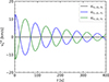	Fig. 5. Similar to Fig. 4 but for the horizontal first overtones of kink oscillations.
In the text

	Fig. 6. Map of the local Alfvén frequency on the y = 0 plane for (a) the fundamental modes and (b) the first overtones. The dashed (dash-dotted) lines represent contours of the frequencies corresponding to the vertical (horizontal) polarizations as labelled.
In the text

	Fig. 7. Initial density distribution along the loop axis. Dashed and dash-doted lines illustrate the function of exp(−z/60) and exp(−z/70), respectively.
In the text

	Fig. 8. Period ratio, Pfun/P1st, as a function of the density stratification, L/πH. The solid curves were derived from Eq. (24). The dashed lines indicate the period ratio of $P_{\mathrm{h}}^{\mathrm{fun}}/P_{\mathrm{h}}^{1\mathrm{st}}$ and $P_{\mathrm{v}}^{\mathrm{fun}}/P_{\mathrm{v}}^{1\mathrm{st}}$ as labelled. See text for more details.
In the text

References

- Andries, J., Arregui, I., & Goossens, M. 2005a, ApJ, 624, L57 [NASA ADS] [CrossRef] [Google Scholar]
- Andries, J., Goossens, M., Hollweg, J. V., Arregui, I., & Van Doorsselaere, T. 2005b, A&A, 430, 1109 [NASA ADS] [CrossRef] [EDP Sciences] [Google Scholar]
- Brady, C. S., & Arber, T. D. 2005, A&A, 438, 733 [NASA ADS] [CrossRef] [EDP Sciences] [Google Scholar]
- Dymova, M. V., & Ruderman, M. S. 2006, A&A, 457, 1059 [NASA ADS] [CrossRef] [EDP Sciences] [Google Scholar]
- Edwin, P. M., & Roberts, B. 1983, Sol. Phys., 88, 179 [Google Scholar]
- Erdélyi, R., & Verth, G. 2007, A&A, 462, 743 [NASA ADS] [CrossRef] [EDP Sciences] [Google Scholar]
- Gao, Y., Van Doorsselaere, T., Tian, H., Guo, M., & Karampelas, K. 2024, A&A, 689, A195 [NASA ADS] [CrossRef] [EDP Sciences] [Google Scholar]
- Gao, Y., Tian, H., Van Doorsselaere, T., et al. 2025, Res. Astron. Astrophys., 25, 015010 [Google Scholar]
- Goossens, M., Hollweg, J. V., & Sakurai, T. 1992, Sol. Phys., 138, 233 [Google Scholar]
- Goossens, M., Andries, J., & Aschwanden, M. J. 2002, A&A, 394, L39 [NASA ADS] [CrossRef] [EDP Sciences] [Google Scholar]
- Guo, M., Li, B., & Van Doorsselaere, T. 2020, ApJ, 904, 116 [Google Scholar]
- Guo, M., Duckenfield, T., Van Doorsselaere, T., et al. 2023, ApJ, 949, L1 [NASA ADS] [CrossRef] [Google Scholar]
- Guo, M., Van Doorsselaere, T., Li, B., & Goossens, M. 2024, A&A, 687, A30 [NASA ADS] [CrossRef] [EDP Sciences] [Google Scholar]
- Karampelas, K., & Van Doorsselaere, T. 2021, ApJ, 908, L7 [NASA ADS] [CrossRef] [Google Scholar]
- Karampelas, K., Van Doorsselaere, T., & Guo, M. 2019, A&A, 623, A53 [NASA ADS] [CrossRef] [EDP Sciences] [Google Scholar]
- Lopin, I., & Nagorny, I. 2024, MNRAS, 527, 5741 [Google Scholar]
- Lopin, I. P., Nagorny, I. G., & Nippolainen, E. 2014, Sol. Phys., 289, 3033 [NASA ADS] [CrossRef] [Google Scholar]
- Magyar, N., & Nakariakov, V. M. 2020, ApJ, 894, L23 [NASA ADS] [CrossRef] [Google Scholar]
- Mignone, A., Bodo, G., Massaglia, S., et al. 2007, ApJS, 170, 228 [Google Scholar]
- Nakariakov, V. M., & Kolotkov, D. Y. 2020, ARA&A, 58, 441 [Google Scholar]
- Nakariakov, V. M., & Ofman, L. 2001, A&A, 372, L53 [NASA ADS] [CrossRef] [EDP Sciences] [Google Scholar]
- Pelouze, G., Van Doorsselaere, T., Karampelas, K., Riedl, J. M., & Duckenfield, T. 2023, A&A, 672, A105 [NASA ADS] [CrossRef] [EDP Sciences] [Google Scholar]
- Reale, F. 2014, Liv. Rev. Sol. Phys., 11, 4 [Google Scholar]
- Ruderman, M. S. 2009, A&A, 506, 885 [NASA ADS] [CrossRef] [EDP Sciences] [Google Scholar]
- Selwa, M., Murawski, K., Solanki, S. K., Wang, T. J., & Tóth, G. 2005, A&A, 440, 385 [NASA ADS] [CrossRef] [EDP Sciences] [Google Scholar]
- Smith, J. M., Roberts, B., & Oliver, R. 1997, A&A, 317, 752 [NASA ADS] [Google Scholar]
- Spruit, H. C. 1981, A&A, 98, 155 [NASA ADS] [Google Scholar]
- Terradas, J., Oliver, R., & Ballester, J. L. 2006, ApJ, 650, L91 [NASA ADS] [CrossRef] [Google Scholar]
- Van Doorsselaere, T., Debosscher, A., Andries, J., & Poedts, S. 2004, A&A, 424, 1065 [NASA ADS] [CrossRef] [EDP Sciences] [Google Scholar]
- Van Doorsselaere, T., Nakariakov, V. M., & Verwichte, E. 2007, A&A, 473, 959 [NASA ADS] [CrossRef] [EDP Sciences] [Google Scholar]
- Van Doorsselaere, T., Verwichte, E., & Terradas, J. 2009, Space Sci. Rev., 149, 299 [NASA ADS] [CrossRef] [Google Scholar]
- Verth, G., & Erdélyi, R. 2008, A&A, 486, 1015 [NASA ADS] [CrossRef] [EDP Sciences] [Google Scholar]
- Verwichte, E., Foullon, C., & Nakariakov, V. M. 2006a, A&A, 446, 1139 [NASA ADS] [CrossRef] [EDP Sciences] [Google Scholar]
- Verwichte, E., Foullon, C., & Nakariakov, V. M. 2006b, A&A, 449, 769 [NASA ADS] [CrossRef] [EDP Sciences] [Google Scholar]
- Verwichte, E., Foullon, C., & Nakariakov, V. M. 2006c, A&A, 452, 615 [NASA ADS] [CrossRef] [EDP Sciences] [Google Scholar]
- Wang, T. J., & Solanki, S. K. 2004, A&A, 421, L33 [NASA ADS] [CrossRef] [EDP Sciences] [Google Scholar]
- Wang, T. J., Solanki, S. K., & Selwa, M. 2008, A&A, 489, 1307 [NASA ADS] [CrossRef] [EDP Sciences] [Google Scholar]
- Yang, Z., Bethge, C., Tian, H., et al. 2020a, Science, 369, 694 [Google Scholar]
- Yang, Z., Tian, H., Tomczyk, S., et al. 2020b, Sci. China E Technol. Sci., 63, 2357 [CrossRef] [Google Scholar]
- Yang, Z., Tian, H., Tomczyk, S., et al. 2024, Science, 386, 76 [Google Scholar]
- Zajtsev, V. V., & Stepanov, A. V. 1975, Issledovaniia Geomagnetizmu Aeronomii i Fizike Solntsa, 37, 3 [NASA ADS] [Google Scholar]
- Zhong, S., Nakariakov, V. M., Kolotkov, D. Y., et al. 2023, Nat. Commun., 14, 5298 [NASA ADS] [CrossRef] [Google Scholar]
- Zimovets, I. V., & Nakariakov, V. M. 2015, A&A, 577, A4 [NASA ADS] [CrossRef] [EDP Sciences] [Google Scholar]