| Issue |
A&A
Volume 707, March 2026
|
|
|---|---|---|
| Article Number | A189 | |
| Number of page(s) | 8 | |
| Section | Cosmology (including clusters of galaxies) | |
| DOI | https://doi.org/10.1051/0004-6361/202558451 | |
| Published online | 05 March 2026 | |
Evidence for dynamical dark energy with an evolving Hubble constant
1
Key Laboratory of Dark Matter and Space Astronomy, Purple Mountain Observatory, Chinese Academy of Sciences Nanjing 210033, PR China
2
School of Astronomy and Space Science, University of Science and Technology of China Hefei Anhui 230026, PR China
★ Corresponding author: This email address is being protected from spambots. You need JavaScript enabled to view it.
Received:
8
December
2025
Accepted:
26
January
2026
Abstract
Context. Hubble constant tension, together with the recent indications of dynamical dark energy proposed from the Dark Energy Spectroscopic Instrument (DESI) baryon acoustic oscillation (BAO) measurements, poses significant challenges for the standard cosmological model.
Aims. We investigate the possible redshift evolution of dark energy and the Hubble constant through a data-driven approach, and assess whether such evolution can alleviate the Hubble constant tension.
Methods. We perform a model-independent reconstruction of the dark-energy equation of state w(z), jointly with an evolving Hubble constant H0(z). The analysis combines the DESI DR2 BAO dataset with multiple Type Ia supernova samples and evaluates the statistical preference for the reconstructed model using Bayesian evidence.
Results. The reconstructed w(z) varies with redshift and exhibits two potential phantom crossings at z ∼ 0.5 and z ∼ 1.5. Meanwhile, H0 decreases continually from local to high redshift, alleviating the Hubble constant tension effectively. The joint w(z)−H0(z) model is favored over the wCDM (ΛCDM) framework, with a logarithmic Bayes factor, ln ℬ = 5.04 (8.53). The results remain stable under different prior choices and dataset combinations.
Conclusions. Our data-driven reconstructions suggest redshift evolution in both w(z) and H0(z), offering a potential route to mitigate the Hubble constant tension. Future BAO measurements from Euclid and next-generation CMB experiments will provide critical tests of these results and bring deeper insights into the nature of dark energy and the evolution of cosmic expansion.
Key words: cosmological parameters / dark energy
© The Authors 2026
 Open Access article, published by EDP Sciences, under the terms of the Creative Commons Attribution License (http://creativecommons.org/licenses/by/4.0), which permits unrestricted use, distribution, and reproduction in any medium, provided the original work is properly cited.
1. Introduction
The standard cosmological paradigm, the cosmological constant Λ and the cold dark matter (ΛCDM) model, successfully explains most cosmological observations. However, the Hubble constant tension and possible evidence for dynamical dark energy pose significant challenges to this standard cosmological framework (Perivolaropoulos & Skara 2022; Abdalla et al. 2022; Di Valentino & Brout 2024; Di Valentino et al. 2025; Wang et al. 2026). Combining Cepheid-based distance measurements from the James Webb Space Telescope (JWST) and the Hubble Space Telescope (HST), Riess et al. (2025) reported a local Hubble constant of H0 = 73.8 ± 0.88 km s−1 Mpc−1 via the distance-ladder method (Riess et al. 2021, 2022), which deviates from the ΛCDM prediction inferred from the cosmic microwave background (CMB) (Planck Collaboration VI 2020) at the ∼6σ confidence level. Meanwhile, the recent baryon acoustic oscillation (BAO) measurements from the Dark Energy Spectroscopic Instrument (DESI) data release 2 (DR2) (DESI Collaboration 2025) prefer a dynamical dark energy model with Chevallier–Polarski–Linder (CPL) parameterization over ΛCDM at a 2.8 − 4.2σ confidence level when combined with CMB and type Ia supernova (SN Ia) data. A ∼5σ level tension has been reported by Scherer et al. (2025) when adopting different parameterization for w(z).
Both the Hubble constant and dark energy govern the accelerating expansion of the Universe, describing its local expansion rate and the physical mechanism behind cosmic acceleration. The dark-energy equation of state (EoS), w ≡ P/c2ρ, serves as a crucial diagnostic: w = −1 corresponds to vacuum energy within the ΛCDM model. For dynamical dark energy, w evolves with time and can be categorized into various models according to their trajectories in the w phase space (Dymnikova & Khlopov 2000, 2001), including quintessence (Ratra & Peebles 1988), phantom (Caldwell 2002), quintom (Feng et al. 2005), k essence (Armendariz-Picon et al. 2000), and others. For the phenomenological quintom model (Feng et al. 2006), an oscillating evolution of w(z) naturally arises, accompanied with a varying H0. Several studies suggest that late-time transitions in dark energy could alleviate the Hubble tension by reducing local H0 values (Benevento et al. 2020; Di Valentino et al. 2021; Pang et al. 2025). However, combining the latest DESI DR2 BAO and CMB data, a lower Hubble constant,  km s−1 Mpc−1, was obtained (DESI Collaboration 2025), thereby exacerbating the Hubble tension. Furthermore, whether current data provide robust evidence for dynamical dark energy remains an open question (Giarè 2025; Ó Colgáin & Sheikh-Jabbari 2025).
To reconcile the discrepancies in Hubble constant measurements between early- and late-time cosmological observations, several studies have constrained H0 by dividing the data into redshift bins. Wong et al. (2020) first reported an apparent trend of decreasing H0 inferred from the individual lensing systems. A possible dynamical evolution of H0 has since been investigated using a phenomenological function (Dainotti et al. 2021, 2022, 2025), modified definitions of the Hubble constant (Krishnan et al. 2021; Jia et al. 2025a), and direct binned measurements (Krishnan et al. 2020; Malekjani et al. 2024; Ó Colgáin et al. 2024; Lopez-Hernandez & De-Santiago 2025). Similarly, the EoS of dark energy, w(z), has been widely reconstructed in redshift bins without imposing an explicit functional form (Zhao et al. 2012, 2017; Abedin et al. 2025). Evidence for the oscillations in w(z) has been found using nonparametric and analytical approaches (Gu et al. 2025; Goldstein et al. 2026), respectively. Given the unknown essence of dark energy remains, such nonparametric, data-driven approaches provide a robust way to trace the evolution of w(z).
In this work, we simultaneously investigate a model-independent dynamical dark energy and an evolving Hubble constant for the first time. We do not assume any specific forms for the dark energy and H0, but instead reconstruct both functions directly from the data using a data-driven approach. The datasets we use include the DESI DR2 BAO measurements (DESI Collaboration 2025), SN Ia observations from the PantheonPlus compilation (Brout et al. 2022; Scolnic et al. 2022), the five-year Dark Energy Survey sample (DESY5) (DES Collaboration 2024), and the Union3 compilation (Rubin et al. 2025). Without assuming any specific functional form, we employed a Gaussian process (GP) to reconstruct w(z) and H0(z) over the redshift range of 0 < z < 2.5. The values of w and H0 are sampled in each redshift bin, enabling a complementary analysis that balances model flexibility and constraining power.
2. Methods
Considering a flat Universe (ΩK = 0), the expansion rate is
![Mathematical equation: $$ \begin{aligned} \frac{H(z)}{H_0(z)} = \left[\Omega _{\rm m} (1+z)^3 + {\Omega _{\rm DE}} \frac{\rho _{\rm DE}(z)}{\rho _{\rm DE,0}}\right]^{1/2}, \end{aligned} $$](/articles/aa/full_html/2026/03/aa58451-25/aa58451-25-eq2.gif) (1)
(1)
where Ωm, ΩDE are the present-time matter and dark energy density parameters, respectively, and H0(z) represents the Hubble parameter evaluated in the corresponding redshift bin. Here, H0(z) can be regarded as an effective, redshift-dependent normalization of the expansion rate, rather than a fundamental Hubble constant. As is shown in Krishnan et al. (2021), the Hubble constant can be represented as an integration constant from the Friedmann equation within the Friedmann–Lemaître–Robertson–Walker metric (FLRW) cosmology. Therefore, Equation (1) reduces to the FLRW framework only when H0(z) is a constant. The energy density, ρDE, that normalized to its present value evolves as
![Mathematical equation: $$ \begin{aligned} \frac{\rho _{\rm DE}(z)}{\rho _{\rm DE,0}} = \mathrm{exp}\left[{3 \int ^z_0[1+w(z)]\frac{\mathrm{d}z\prime }{1+z\prime }}\right]. \end{aligned} $$](/articles/aa/full_html/2026/03/aa58451-25/aa58451-25-eq3.gif) (2)
(2)
The contributions from radiation and massive neutrinos are neglected for simplification. The BAO distance observables include the comoving distance, DM(z), the Hubble distance, DH(z), and the angle-average distance, DV(z), which can be written as
 (3)
(3)
and DV(z) = (zDM(z)2DH(z))1/3.
The pre-recombination sound horizon at the drag epoch is defined as rd = ∫zd∞cs(z)/H(z)dz, where cs is the sound speed in the primordial plasma. Following Brieden et al. (2023) and DESI Collaboration (2025), it can be approximated as
 (4)
(4)
where h ≡ H0, z = 0/(100 km s−1 Mpc−1) and Neff is the effective number of neutrino species. In this work, only the variations in Ωb and Ωm are considered. The DESI DR2 BAO data cover 0.1 < z < 4.2 using multiple tracers: the bright galaxy sample (0.1 < z < 0.4), luminous red galaxies (0.4 < z < 1.1), emission line galaxies (1.1 < z < 1.6), quasars (0.8 < z < 2.1), and a Lyα forest (1.77 < z < 4.16). For the SN Ia samples, the PantheonPlus compilation1 (Brout et al. 2022; Scolnic et al. 2022) contains 1701 light curves of 1550 distinct SNe Ia covering 0.001 < z < 2.26, the DESY5 sample (DES Collaboration 2024) includes 1635 SNe Ia within 0.10 < z < 1.13, and the Union3 compilation2 (Rubin et al. 2025) provides 2087 SNe Ia covering 0.001 < z < 2.26. We used the observations that satisfy z > 0.01. The luminosity distance is given by DL(z) = (1 + z)DM(z).
We modeled the evolution of w(z) and H0(z) over the redshift range 0 < z < 2.5. The upper bound of z = 2.5 is a conservative choice that encompasses all the observational datasets used in this analysis. The target range was divided into 29 bins of uniform width in the scale factor (a = 1/(1 + z)) space (Gu et al. 2025). To reconstruct smooth and continuous functions of w(z) and H0 without assuming any explicit functional form, we employed the GP as a nonparametric statistical method. The GP has been extensively applied in data-driven astronomy (Holsclaw et al. 2010; Shafieloo et al. 2012; Li et al. 2021), demonstrating powerful strength to sample the space of continuous functions. For prior assumptions, we adopted three types of kernels and methods to construct the covariance matrices, Σ: the Matérn kernel, KMatérn(δa, ν, l), Gaussian kernel, KGaussian(δa, l), and Horndeski theory (Horndeski 1974). The general form of the covariance matrix is Σij = σ2K(|ai − aj|,l), where σ represents the amplitude of the function, ai denotes the median point of the i-th bin in scale factor space, and l governs the correlation length scale. For the Horndeski-based covariance, we adopted the prior covariance from Horndeski-based simulations (Raveri et al. 2017), expressed as
![Mathematical equation: $$ \begin{aligned} \begin{aligned} C(a_i, \, a_j)&= \sqrt{C(a_i) C(a_j)} R(a_i, \, a_j), \\ C(a_i)&=0.05 + 0.8a_i^2, \\ R(a_i, \, a_j)&= \exp {\left[-(|\ln a_i - \ln a_j|/0.3)^{1.2}\right]}. \end{aligned} \end{aligned} $$](/articles/aa/full_html/2026/03/aa58451-25/aa58451-25-eq6.gif) (5)
(5)
Following Gu et al. (2025), the covariance matrix, Σ, was calculated as
![Mathematical equation: $$ \begin{aligned} \mathbf \Sigma = \left[(\mathbf I - \mathbf S )^{T} \mathbf{C }^{-1} (\mathbf I - \mathbf S )\right]^{-1}, \end{aligned} $$](/articles/aa/full_html/2026/03/aa58451-25/aa58451-25-eq7.gif) (6)
(6)
where I is the identity matrix and S is the transformation matrix that averages over five neighboring w bins. The Horndeski-based covariance matrix predicts a variable σ(w) ranging from 1.6 to 6.2 across bins. Accordingly, we adopted a constant σ(w) = 3 for both the Matérn and Gaussian kernels, in order to ensure a consistent comparison across different kernel and model assumptions. For the H0(z) reconstruction, we set σ(H0) = 15 as a weakly informative prior in the Bayesian inference, ensuring that the reconstructed evolution of H0(z) is driven primarily by the data rather than by prior assumptions. The mean values are assumed to be μ(H0) = 70 and μ(w) = − 1, respectively. In this work, it should be noticed that GPs are employed as functional priors on w(z) and H0(z), rather than as a direct interpolation technique. The correlation length, l, was not optimized by maximizing or marginalizing GP likelihoods. Instead, we scanned a range of fixed values and assessed their performance by comparing the Bayesian evidence of the full cosmological model. We applied a flat prior on Ωm and a Gaussian prior on Ωb, with Ωm ∈ [0.1, 0.5] and Ωbh2 = 0.02196 ± 0.00063 (Schöneberg 2024). Additional constraints require H0(z) and w(z) to remain within [50, 90] and [−6, 4], respectively.
Since all of the components involved in the DESI BAO and SNe Ia measurements have been explicitly implemented, the likelihood functions in the Bayesian statistical framework can be written as
![Mathematical equation: $$ \begin{aligned} \begin{aligned} \mathcal{L} _{\rm BAO}&=\prod ^{N}_{i} \mathrm{exp} \left[-\frac{1}{2} \left(\frac{f(x_i)-y_i}{\sigma _i}\right)^2\right],\\ \mathcal{L} _{\rm SNe}&= \mathrm{exp}\left[-\frac{1}{2}{\Delta }{{\boldsymbol{D}}}^{T} C^{-1}_{\rm stat+syst}{\Delta }{{\boldsymbol{D}}}\right], \end{aligned} \end{aligned} $$](/articles/aa/full_html/2026/03/aa58451-25/aa58451-25-eq8.gif) (7)
(7)
where (xi, yi) and σi are the DESI BAO measurements and their uncertainties, D is the vector of SNe Ia distance modulus residuals, defined as ΔDi = μi − μmodel(zi), and Cstat + syst denotes the statistical and systematic covariance matrices. To balance the efficiency and accuracy, we employed the nested sampling algorithm implemented in pymultinest (Buchner 2016) and set 2000 live points during Bayesian analysis.
3. Results
The evolutions of w(z) and H0(z) were reconstructed simultaneously. Each was divided into 29 bins. The priors of w = (w1, …, w29) and H0 = (H0, 1, …, H0, 29) were generated either from the Horndeski theory or from the GP kernel functions, expressed as π(w|μ, σ, l) and π(H0|μ, σ, l), respectively. Besides σ, the length scale, l, acts as another hyperparameter that regulates the smoothness of reconstructed functions. Larger l values enforce stronger correlations, stiffening the model that will ignore the details, while smaller l values soften the model but may risk overfitting. We compare Bayesian evidences across several configurations with different l values and find that H0(z) shows a clear decreasing trend. This preference for a smoother function for H0(z) leads us to adopt a Gaussian kernel with a relatively large length scale. Detailed comparisons of the scale length are provided in Section 4.
Figure 1 illustrates the reconstructed w(z) (top panels) and H0(z) (bottom panels) derived from various data combinations. The priors of w were generated using the Matérn-3/2 kernel with l = 2.5 and ν = 2/3 for the DESI + PantheonPlus and DESI + DESY5 datasets, and l = 0.9 for the DESI + Union3 case. The priors of H0 were generated using the Gaussian kernel with l = 2.0. These configurations yield the highest Bayesian evidence among all tested l values, rather than being fit through a GP or marginal likelihood optimization. In all cases, w(z) exhibits clear redshift evolution with multiple peaks, while H0(z) demonstrates a significant decreasing trend from ∼73 to ∼70 km s−1 Mpc−1, approaching the CMB-inferred value. To quantify the model preference for dynamical dark energy and an evolving Hubble constant, we computed the Bayes factor,  . The priors of the wCDM model are consistent with those described previously. From left to right in Figure 1, we obtained ln ℬ = 4.18, 3.39, and 2.13, respectively. Compared with ΛCDM models, Bayes factors give ln ℬ = 0.69, 7.67, and 1.54, respectively. As was pointed out by Jeffreys (1939), ln ℬ > 2.3 (ln ℬ > 3.5) indicates a strong (very strong) preference for one model over another, and ln ℬ > 4.6 is regarded as decisive evidence. Thus, the DESI + PantheonPlus and DESI + DESY5 datasets provide very strong and strong support for the joint w(z)−H0(z) model, respectively.
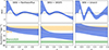 |
Fig. 1. Reconstructed dark-energy EoS, w(z), and Hubble constant, H0(z), from multiple datasets. The GP priors for w(z) and H0(z) use Matérn-3/2 and Gaussian kernels, respectively. The panels in each column correspond to using the same datasets. Solid blue lines show the mean values of the w(z) and H0(z) distributions. The shaded blue regions indicate the corresponding 68% credible intervals. The dashed black lines marks w = −1. The orange and green bands denote H0 estimations from SNe Ia (Riess et al. 2022) and the CMB (Planck Collaboration VI 2020), respectively. |
As a robustness test, the results using Gaussian kernels and Horndeski theory are shown in Figures 2 and 3, respectively. The priors of H0 were generated using the Gaussian kernel with l = 2.0, except for the middle and right panels in Figure 3, which use a Gaussian kernel with l = 1.0. The Gaussian kernel yields smoother reconstructions with a larger length scale, whereas the Matérn kernel allows for greater flexibility. The Horndeski prior produces the most flexible w(z) evolution, capturing more distinct features in the observations. In Figure 2, the blue regions correspond to the priors of w that are generated by the Gaussian kernel with l = 0.2 for DESI + PantheonPlus and DESI + DESY5, and l = 0.05 for the DESI + Union3 scenarios. The resulting Bayes factors relative to wCDM (ΛCDM) model are ln ℬ = 3.74 (0.23), 2.96 (7.24), and 2.86 (2.27), respectively, again showing a very strong preference for DESI + PantheonPlus and a strong preference for other datasets. The purple regions in the right panels represent reconstructions with l = 0.2, yielding consistent shapes compared with other scenarios using different datasets but a smaller ln ℬ = 0.64. For the results using the Horndeski prior shown in Figure 3, Bayes factors relative to wCDM (ΛCDM) model are ln ℬ = 5.04 (1.55), 4.25 (8.53), and 3.06 (2.47) for different datasets, respectively. Notably, the DESI + PantheonPlus combination provides a decisive evidence (ln ℬ > 4.6) favoring the w(z)−H0(z) model.
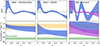 |
Fig. 2. Reconstructed dark-energy EoS, w(z), and Hubble constant, H0(z). Similar to Figure 1, but adopting a Gaussian kernel to define the GP prior covariance for w(z). In the right panel, the blue region represents the results with a maximum Bayes factor with l = 0.05. The purple region corresponds to l = 0.2, assuming the same scale length as in the left and middle panels. A smaller l (l < 0.01) in the DESI + Union case may yield stronger Bayesian evidence, but the resulting w(z) becomes too flexible to provide a clear constraint. Therefore, the right panel only shows the results for l = 0.05 and l = 0.2. |
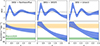 |
Fig. 3. Reconstructed dark-energy EoS, w(z), and Hubble constant, H0(z). Similar to Figure 1, but using the Horndeski theory to derive the w(z) prior. The results in the left panel use a Gaussian kernel with l = 2.0 to derive the H0(z) priors, while the others use l = 1.0 to obtain the maximum Bayes factors. |
All nine scenarios, constructed with different dataset combinations and prior assumptions, consistently indicate that both the dark-energy EoS, w(z), and the Hubble constant, H0, can evolve with redshift. Compared with Equations (1) and (2), the evolved H0 suggests that dynamical dark energy alone may not be sufficient to fully explain the Hubble constant tension, potentially indicating the presence of new physics beyond the standard cosmological model. Several deviations from the ΛCDM model appear at distinct epochs. The reconstructed w(z) crosses into the phantom regime (w < −1) around z ≈ 0.5, consistent with previous nonparametric DESI BAO analyses (Lodha et al. 2025). It returns to the quintessence regime around z ≈ 1.0, and then crosses again into the phantom region near z ≈ 1.5. Particularly, all reconstructions show a preference for w(z) exhibiting two phantom crossings. Furthermore, no clear non-monotonic behavior is observed in H0(z). Instead, all results present a gradual decline from local to higher redshift, with different amplitudes depending on the dataset and prior choice. The DESI + PantheonPlus case with a Gaussian kernel yields the smallest variation, from  to
to  km s−1 Mpc−1, while the DESI + DESY5 case with the Horndeski theory gives the largest one, from
  to
to  km s−1 Mpc−1. Compared with the results based on the classical CPL parameterization (DESI Collaboration 2025), a lower H0 value is typically obtained when w0 > −1, as a consequence of parameter degeneracy inherent in the CPL model (Lee et al. 2022). Differently, our result alleviates the Hubble constant tension through the downward evolution of H0(z), enabled by a dynamical dark energy with greater freedom than the CPL parameterization.
4. Conclusions and discussions
In this work, we have reconstructed the dynamical dark-energy EoS, w(z), together with an evolving Hubble constant, H0(z), with nonparametric methods. Across multiple dataset combinations and prior assumptions, we find consistent evolution patterns: w(z) evolves with redshift and emerges into two potential phantom crossing, and H0(z) decreases smoothly toward high redshift. In particular, the DESI + DESY5 scenario with the Horndeski prior gives the largest downward trend, ΔH0 ∼ 8.4 km s−1 kpc−1, reaching H0 ∼ 67.4 km s−1 Mpc. Compared with the wCDM model and the ΛCDM model (w = −1), the Bayes factors are ln ℬ = 4.25 and 8.53, respectively, providing a promising solution to relieve the Hubble constant tension. Furthermore, the maximum Bayes factor among all scenarios compared with the wCDM model reaches ln ℬ = 5.04, establishing decisive evidence for w(z)−H0(z) model.
The above results and discussions depend on the choice of the characteristic scale length, l. To clarify the selection of l in each case, we compared the Bayes factors relative to the wCDM model for different scale factors, l, across multiple scenarios. As is shown in Figure 4, the panels from left to right display the variations of ln ℬ in the reconstructions of w(z) using Matérn-3/2 and Gaussian kernels, and of the H0(z) using Gaussian kernels. In the left and middle panels, the priors of H0(z) were generated with a Gaussian kernel of l = 2.0, while in the right panel, the priors of w(z) were derived from the Horndeski theory and the priors of H0(z) were constructed with a Gaussian kernel using variable l. The variations of ln ℬ in the middle panel exhibit a moderate increase with larger l, which may result from the reduced effective degrees of freedom introduced by smoother Gaussian-kernel priors. The maximum values of ln ℬ correspond to the results presented in Section 3. Detailed parameter estimation results are listed in Appendix A.
 |
Fig. 4. Comparisons with different scale lengths under various prior assumptions. The red, orange, and blue scatters represent the Bayes factors relative to wCDM models using DESI combined with the PantheonPlus, DESY5, and Union3 datasets, respectively. |
Given that measurements of BAOs rely on the pre-recombination sound-horizon scale and the degeneracy between rd and H0, we examined the impact of rd on the constructions of w(z) and H0(z). Instead of adopting the fixed relation in Equation (4), we assumed rd to be a free parameter with a uniform prior of [120, 180] Mpc. Figure 5 shows the results using the DESI + PantheonPlus datasets. The reconstructed w(z) remains consistent with previous cases, and H0(z) continues to exhibit the same decreasing trend. As was expected, the uncertainties in H0(z) increase because BAO measurements constrain the product H0rd more tightly than the individual parameters (DESI Collaboration 2025). For example, under the Horndeski prior, H0 declines from  to
to  km s−1 kpc−1. Three different prior assumptions were used, including the Matérn-3/2 kernel, the Gaussian kernel with l = 0.2, and the Horndeski theory. The Bayes factors relative to the wCDM model are ln ℬ = 3.17, 2.66, and 4.02, respectively, corresponding to two strong preferences for the w(z)−H0(z) framework and one very strong preference.
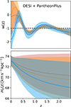 |
Fig. 5. Reconstructions of w(z) and H0(z) using the DESI + PantheonPlus datasets. The prior of H0(z) uses the Gaussian kernel with l = 1.5. The shaded regions indicate the corresponding 68% credible intervals. The red, orange, and blue regions correspond to w(z) priors generated from the Matérn-3/2 kernel (l = 2.5), the Gaussian kernel (l = 0.2), and the Horndeski theory, respectively. |
The reconstruction of w(z) using both Matérn-3/2 and Gaussian kernels shows consistent results with the Horndeski prior, particularly the evidence of two phantom crossings. Based on independent analyses, Gu et al. (2025) and Goldstein et al. (2026) have reported oscillatory features in w(z) consistent with our results. To validate the reconstruction method, we performed the same procedure using the simulated data with observational uncertainties matching those of PantheonPlus and DESI DR2. As is shown in Figure 6, both the CPL parameterization and the oscillation model can be accurately reconstructed using the same kernel function. For the scenario using the CPL parameterization, no pseudo oscillation arises, demonstrating the robustness of our method and the reliability of the physical transition signatures identified in our results.
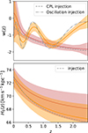 |
Fig. 6. Reconstructions of w(z) and H0(z) based on simulated injection. The gray lines denote the injected models. For w(z), the dashed gray line represents the CPL parameterization with w(z) = − 0.5 − 2(1 − 1/(1 + z)) and the dash-dotted gray line shows the oscillation model with w(z) = 0.8 sin[20(1 − 1/(1 + z))]−1. For simplicity, the other injected parameters are fixed with Ωm = 0.3, ωbh2 = 0.02196, and Mb = −19.5. For H0(z), the dashed gray line corresponds to H0(z) = 73 − 9.8(1 − 1/(1 + z)). The shaded regions indicate the corresponding 90% credible intervals. The prior of H0(z) uses the Gaussian kernel with l = 2.0, and the prior of w(z) was generated from the Matérn-3/2 kernel (l = 2.5). |
As one of the most general scalar-tensor theories involving second-order field equations, the Horndeski framework has been widely investigated for its potential to alleviate the Hubble tension by predicting a large H0 (Petronikolou et al. 2022; Banerjee et al. 2023; Tiwari et al. 2024). After defining the effective Hubble parameters through the expansion rate of ΛCDM and wCDM models, Montani et al. (2025) and Jia et al. (2025b) proposed that a running H0 naturally arises from evolving dark energy. Because phantom-crossing behavior can drive a faster expansion phase, leading to large H0, the concept of an evolved H0(z) is theoretically motivated. Furthermore, our reconstructions of w(z) are compatible with various dynamical dark-energy models. If dark energy can possess multiple internal degrees of freedom, such as multi-field models (Hu 2005; Guo et al. 2005; Cai et al. 2008), modified vacuum models (Parker & Raval 2000; Caldwell et al. 2006), and interacting dark-energy models (Billyard & Coley 2000), phantom crossing can be generated properly.
Beyond traditional approaches, many novel astrophysical probes covering a broad range of redshifts have been proposed to measure the cosmological parameters and the dark-energy EoS. For instance, the spectral peaks of gamma-ray bursts (merger events via gravitational-wave observations) can serve as tracers (standard sirens) of cosmic expansion (Dai et al. 2004; Abbott et al. 2017; Wang et al. 2023; Li et al. 2024), the dispersion measures of fast radio bursts provide independent constraints on H0 and w(z) (Zhou et al. 2014; Wang et al. 2025), and the propagation speed of gravitational waves from multi-messenger events can test large classes of scalar-tensor and dark-energy theories (Ezquiaga & Zumalacárregui 2017). In addition to w(z) and H0, several other cosmological parameters have been modeled as redshift-dependent functions to explain current cosmological tensions (Ó Colgáin et al. 2022; Fazzari et al. 2026; Ó Colgáin et al. 2024). Looking forward, next-generation CMB experiments (CMB-S4, the Simons Observatory, and LiteBIRD) (Abazajian et al. 2022; Lee et al. 2019; LiteBIRD Collaboration 2023), together with high-precision BAO surveys such as Euclid (Euclid Collaboration: Mellier et al. 2025), will substantially tighten cosmological constraints and provide crucial insights into the physics of dark energy and cosmic expansion.
Acknowledgments
We thank the anonymous referee for helpful comments and suggestions. This work is supported in part by NSFC under grants of No. 12233011, the Postdoctoral Fellowship Program of CPSF (No. GZB20250738), and the Jiangsu Funding Program for Excellent Postdoctoral Talent (No. 2025ZB209).
References
- Abazajian, K., Abdulghafour, A., Addison, G. E., et al. 2022, ArXiv e-prints [arXiv:2203.08024] [Google Scholar]
- Abbott, B. P., Abbott, R., Abbott, T. D., et al. 2017, Nature, 551, 85 [Google Scholar]
- Abdalla, E., Abellán, G. F., Aboubrahim, A., et al. 2022, J. High Energy Astrophys., 34, 49 [NASA ADS] [CrossRef] [Google Scholar]
- Abedin, M., Wang, G.-J., Ma, Y.-Z., & Pan, S. 2025, MNRAS, 540, 2253 [Google Scholar]
- Armendariz-Picon, C., Mukhanov, V., & Steinhardt, P. J. 2000, Phys. Rev. Lett., 85, 4438 [Google Scholar]
- Banerjee, S., Petronikolou, M., & Saridakis, E. N. 2023, Phys. Rev. D, 108, 024012 [Google Scholar]
- Benevento, G., Hu, W., & Raveri, M. 2020, Phys. Rev. D, 101, 103517 [Google Scholar]
- Billyard, A. P., & Coley, A. A. 2000, Phys. Rev. D, 61, 083503 [Google Scholar]
- Brieden, S., Gil-Marín, H., & Verde, L. 2023, JCAP, 2023, 023 [CrossRef] [Google Scholar]
- Brout, D., Scolnic, D., Popovic, B., et al. 2022, ApJ, 938, 110 [NASA ADS] [CrossRef] [Google Scholar]
- Buchner, J. 2016, Astrophysics Source Code Library [record ascl:1606.005] [Google Scholar]
- Cai, Y.-F., Qiu, T., Brandenberger, R., Piao, Y.-S., & Zhang, X. 2008, JCAP, 2008, 013 [Google Scholar]
- Caldwell, R. R. 2002, Phys. Lett. B, 545, 23 [Google Scholar]
- Caldwell, R. R., Komp, W., Parker, L., & Vanzella, D. A. T. 2006, Phys. Rev. D, 73, 023513 [Google Scholar]
- Dai, Z. G., Liang, E. W., & Xu, D. 2004, ApJ, 612, L101 [NASA ADS] [CrossRef] [Google Scholar]
- Dainotti, M. G., De Simone, B., Schiavone, T., et al. 2021, ApJ, 912, 150 [NASA ADS] [CrossRef] [Google Scholar]
- Dainotti, M. G., De Simone, B. D., Schiavone, T., et al. 2022, Galaxies, 10, 24 [NASA ADS] [CrossRef] [Google Scholar]
- Dainotti, M. G., De Simone, B., Garg, A., et al. 2025, J. High Energy Astrophys., 48, 100405 [Google Scholar]
- DES Collaboration (Abbott, T. M. C., et al.) 2024, ApJ, 973, L14 [NASA ADS] [CrossRef] [Google Scholar]
- DESI Collaboration (Abdul-Karim, M., et al.) 2025, Phys. Rev. D, 112, 083515 [Google Scholar]
- Di Valentino, E., & Brout, D. 2024, The Hubble Constant Tension (Springer) [Google Scholar]
- Di Valentino, E., Mukherjee, A., & Sen, A. A. 2021, Entropy, 23, 404 [Google Scholar]
- Di Valentino, E., Said, J. L., Riess, A., et al. 2025, Phys. Dark Univ., 49, 101965 [Google Scholar]
- Dymnikova, I., & Khlopov, M. 2000, Mod. Phys. Lett. A, 15, 2305 [Google Scholar]
- Dymnikova, I., & Khlopov, M. 2001, Eur. Phys. J. C, 20, 139 [Google Scholar]
- Euclid Collaboration (Mellier, Y., et al.) 2025, A&A, 697, A1 [Google Scholar]
- Ezquiaga, J. M., & Zumalacárregui, M. 2017, Phys. Rev. Lett., 119, 251304 [NASA ADS] [CrossRef] [Google Scholar]
- Fazzari, E., Giarè, W., & Di Valentino, E. 2026, ApJ, 996, L5 [Google Scholar]
- Feng, B., Wang, X., & Zhang, X. 2005, Phys. Lett. B, 607, 35 [Google Scholar]
- Feng, B., Li, M., Piao, Y.-S., & Zhang, X. 2006, Phys. Lett. B, 634, 101 [Google Scholar]
- Giarè, W. 2025, Phys. Rev. D, 112, 023508 [Google Scholar]
- Goldstein, S., Celoria, M., & Schmidt, F. 2026, Phys. Rev., 113, 023532 [Google Scholar]
- Gu, G., Wang, X., Wang, Y., et al. 2025, Nat. Astron., 9, 1879 [Google Scholar]
- Guo, Z.-K., Piao, Y.-S., Zhang, X., & Zhang, Y.-Z. 2005, Phys. Lett. B, 608, 177 [Google Scholar]
- Holsclaw, T., Alam, U., Sansó, B., et al. 2010, Phys. Rev. Lett., 105, 241302 [NASA ADS] [CrossRef] [Google Scholar]
- Horndeski, G. W. 1974, Int. J. Theor. Phys., 10, 363 [NASA ADS] [CrossRef] [Google Scholar]
- Hu, W. 2005, Phys. Rev. D, 71, 047301 [Google Scholar]
- Jeffreys, H. 1939, Theory of Probability (Oxford: Oxford University Press) [Google Scholar]
- Jia, X. D., Hu, J. P., Yi, S. X., & Wang, F. Y. 2025a, ApJ, 979, L34 [Google Scholar]
- Jia, X. D., Hu, J. P., Gao, D. H., Yi, S. X., & Wang, F. Y. 2025b, ApJ, 994, L22 [Google Scholar]
- Krishnan, C., Ó Colgáin, E., Ruchika, S., et al. 2020, Phys. Rev. D, 102, 103525 [NASA ADS] [CrossRef] [Google Scholar]
- Krishnan, C., Ó Colgáin, E., Sheikh-Jabbari, M. M., & Yang, T. 2021, Phys. Rev. D, 103, 103509 [NASA ADS] [CrossRef] [Google Scholar]
- Lee, A., Abitbol, M. H., Adachi, S., et al. 2019, BAAS, 51, 147 [NASA ADS] [Google Scholar]
- Lee, B.-H., Lee, W., Ó Colgáin, E., Sheikh-Jabbari, M. M., & Thakur, S. 2022, JCAP, 2022, 004 [CrossRef] [Google Scholar]
- Li, Y.-J., Wang, Y.-Z., Han, M.-Z., et al. 2021, ApJ, 917, 33 [NASA ADS] [CrossRef] [Google Scholar]
- Li, Y.-J., Tang, S.-P., Wang, Y.-Z., & Fan, Y.-Z. 2024, ApJ, 976, 153 [Google Scholar]
- LiteBIRD Collaboration (Allys, E., et al.) 2023, Progr. Theor. Exp. Phys., 2023, 042F01 [CrossRef] [Google Scholar]
- Lodha, K., Calderon, R., Matthewson, W. L., et al. 2025, Phys. Rev. D, 112, 083511 [Google Scholar]
- Lopez-Hernandez, M., & De-Santiago, J. 2025, JCAP, 2025, 026 [Google Scholar]
- Malekjani, M., Mc Conville, R., Ó Colgáin, E., Pourojaghi, S., & Sheikh-Jabbari, M. M. 2024, Eur. Phys. J. C, 84, 317 [NASA ADS] [CrossRef] [Google Scholar]
- Montani, G., Carlevaro, N., & Dainotti, M. G. 2025, Phys. Dark Univ., 48, 101847 [Google Scholar]
- Ó Colgáin, E., & Sheikh-Jabbari, M. M. 2025, MNRAS, 542, L24 [Google Scholar]
- Ó Colgáin, E., Sheikh-Jabbari, M. M., Solomon, R., et al. 2022, Phys. Rev. D, 106, L041301 [CrossRef] [Google Scholar]
- Ó Colgáin, E., Sheikh-Jabbari, M. M., Solomon, R., Dainotti, M. G., & Stojkovic, D. 2024, Phys. Dark Univ., 44, 101464 [Google Scholar]
- Pang, Y.-H., Zhang, X., & Huang, Q.-G. 2025, Sci. China Phys. Mech. Astron., 68, 280410 [Google Scholar]
- Parker, L., & Raval, A. 2000, Phys. Rev. D, 62, 083503 [Google Scholar]
- Perivolaropoulos, L., & Skara, F. 2022, New Astron. Rev., 95, 101659 [CrossRef] [Google Scholar]
- Petronikolou, M., Basilakos, S., & Saridakis, E. N. 2022, Phys. Rev. D, 106, 124051 [Google Scholar]
- Planck Collaboration VI. 2020, A&A, 641, A6 [NASA ADS] [CrossRef] [EDP Sciences] [Google Scholar]
- Ratra, B., & Peebles, P. J. E. 1988, Phys. Rev. D, 37, 3406 [Google Scholar]
- Raveri, M., Bull, P., Silvestri, A., & Pogosian, L. 2017, Phys. Rev. D, 96, 083509 [Google Scholar]
- Riess, A. G., Casertano, S., Yuan, W., et al. 2021, ApJ, 908, L6 [NASA ADS] [CrossRef] [Google Scholar]
- Riess, A. G., Yuan, W., Macri, L. M., et al. 2022, ApJ, 934, L7 [NASA ADS] [CrossRef] [Google Scholar]
- Riess, A. G., Li, S., Anand, G. S., et al. 2025, ApJ, 992, L34 [Google Scholar]
- Rubin, D., Aldering, G., Betoule, M., et al. 2025, ApJ, 986, 231 [Google Scholar]
- Scherer, M., Sabogal, M. A., Nunes, R. C., & De Felice, A. 2025, Phys. Rev. D, 112, 043513 [Google Scholar]
- Schöneberg, N. 2024, JCAP, 2024, 006 [Google Scholar]
- Scolnic, D., Brout, D., Carr, A., et al. 2022, ApJ, 938, 113 [NASA ADS] [CrossRef] [Google Scholar]
- Shafieloo, A., Kim, A. G., & Linder, E. V. 2012, Phys. Rev. D, 85, 123530 [CrossRef] [Google Scholar]
- Tiwari, Y., Ghosh, B., & Jain, R. K. 2024, Eur. Phys. J. C, 84, 220 [Google Scholar]
- Wang, Y.-Y., Tang, S.-P., Jin, Z.-P., & Fan, Y.-Z. 2023, ApJ, 943, 13 [NASA ADS] [CrossRef] [Google Scholar]
- Wang, Y.-Y., Gao, S.-J., & Fan, Y.-Z. 2025, ApJ, 981, 9 [Google Scholar]
- Wang, Y.-Y., Lei, L., Tang, S.-P., & Fan, Y.-Z. 2026, JCAP, 2026, 009 [Google Scholar]
- Wong, K. C., Suyu, S. H., Chen, G. C. F., et al. 2020, MNRAS, 498, 1420 [Google Scholar]
- Zhao, G.-B., Crittenden, R. G., Pogosian, L., & Zhang, X. 2012, Phys. Rev. Lett., 109, 171301 [NASA ADS] [CrossRef] [Google Scholar]
- Zhao, G.-B., Raveri, M., Pogosian, L., et al. 2017, Nat. Astron., 1, 627 [NASA ADS] [CrossRef] [Google Scholar]
- Zhou, B., Li, X., Wang, T., Fan, Y.-Z., & Wei, D.-M. 2014, Phys. Rev. D, 89, 107303 [NASA ADS] [CrossRef] [Google Scholar]
We use the PantheonPlus compilation accompanied by the SH0ES Cepheids, obtained from https://github.com/PantheonPlusSH0ES/
The likelihoods of the DESY5 and Union3 compilations are calculated by the cosmological inference software cobaya (https://github.com/CobayaSampler).
Appendix A: The results of parameter estimations for various cosmological models
This appendix presents the posterior distributions of the cosmological parameters and the corresponding Bayesian evidences for all scenarios discussed in the main text. For the reconstructions of H0(z), we show the values at z ∼ 0.01 and z ∼ 0.36. For w(z), the specific and local extreme values are listed.
‘D+P’, ‘D+D’, and ‘D+U’ represents the data combinations of DESI + Pantheon, DESI + DESY5, and DESI + Union, respectively. ‘M’, ‘G’, and ‘U’ represent the cases that the priors of w(z) are derived using the Matérn-3/2 kernel, the Gaussian kernels, and the Horndeski theory. ln(E) denotes the Bayesian evidence corresponding to each case.
All Tables
‘D+P’, ‘D+D’, and ‘D+U’ represents the data combinations of DESI + Pantheon, DESI + DESY5, and DESI + Union, respectively. ‘M’, ‘G’, and ‘U’ represent the cases that the priors of w(z) are derived using the Matérn-3/2 kernel, the Gaussian kernels, and the Horndeski theory. ln(E) denotes the Bayesian evidence corresponding to each case.
All Figures
|
Fig. 1. Reconstructed dark-energy EoS, w(z), and Hubble constant, H0(z), from multiple datasets. The GP priors for w(z) and H0(z) use Matérn-3/2 and Gaussian kernels, respectively. The panels in each column correspond to using the same datasets. Solid blue lines show the mean values of the w(z) and H0(z) distributions. The shaded blue regions indicate the corresponding 68% credible intervals. The dashed black lines marks w = −1. The orange and green bands denote H0 estimations from SNe Ia (Riess et al. 2022) and the CMB (Planck Collaboration VI 2020), respectively. |
| In the text | |
|
Fig. 2. Reconstructed dark-energy EoS, w(z), and Hubble constant, H0(z). Similar to Figure 1, but adopting a Gaussian kernel to define the GP prior covariance for w(z). In the right panel, the blue region represents the results with a maximum Bayes factor with l = 0.05. The purple region corresponds to l = 0.2, assuming the same scale length as in the left and middle panels. A smaller l (l < 0.01) in the DESI + Union case may yield stronger Bayesian evidence, but the resulting w(z) becomes too flexible to provide a clear constraint. Therefore, the right panel only shows the results for l = 0.05 and l = 0.2. |
| In the text | |
|
Fig. 3. Reconstructed dark-energy EoS, w(z), and Hubble constant, H0(z). Similar to Figure 1, but using the Horndeski theory to derive the w(z) prior. The results in the left panel use a Gaussian kernel with l = 2.0 to derive the H0(z) priors, while the others use l = 1.0 to obtain the maximum Bayes factors. |
| In the text | |
|
Fig. 4. Comparisons with different scale lengths under various prior assumptions. The red, orange, and blue scatters represent the Bayes factors relative to wCDM models using DESI combined with the PantheonPlus, DESY5, and Union3 datasets, respectively. |
| In the text | |
|
Fig. 5. Reconstructions of w(z) and H0(z) using the DESI + PantheonPlus datasets. The prior of H0(z) uses the Gaussian kernel with l = 1.5. The shaded regions indicate the corresponding 68% credible intervals. The red, orange, and blue regions correspond to w(z) priors generated from the Matérn-3/2 kernel (l = 2.5), the Gaussian kernel (l = 0.2), and the Horndeski theory, respectively. |
| In the text | |
|
Fig. 6. Reconstructions of w(z) and H0(z) based on simulated injection. The gray lines denote the injected models. For w(z), the dashed gray line represents the CPL parameterization with w(z) = − 0.5 − 2(1 − 1/(1 + z)) and the dash-dotted gray line shows the oscillation model with w(z) = 0.8 sin[20(1 − 1/(1 + z))]−1. For simplicity, the other injected parameters are fixed with Ωm = 0.3, ωbh2 = 0.02196, and Mb = −19.5. For H0(z), the dashed gray line corresponds to H0(z) = 73 − 9.8(1 − 1/(1 + z)). The shaded regions indicate the corresponding 90% credible intervals. The prior of H0(z) uses the Gaussian kernel with l = 2.0, and the prior of w(z) was generated from the Matérn-3/2 kernel (l = 2.5). |
| In the text | |
Current usage metrics show cumulative count of Article Views (full-text article views including HTML views, PDF and ePub downloads, according to the available data) and Abstracts Views on Vision4Press platform.
Data correspond to usage on the plateform after 2015. The current usage metrics is available 48-96 hours after online publication and is updated daily on week days.
Initial download of the metrics may take a while.