| Issue |
A&A
Volume 707, March 2026
|
|
|---|---|---|
| Article Number | A127 | |
| Number of page(s) | 13 | |
| Section | Planets, planetary systems, and small bodies | |
| DOI | https://doi.org/10.1051/0004-6361/202558469 | |
| Published online | 10 March 2026 | |
Precomputed aerosol extinction, scattering, and asymmetry grids for scalable atmospheric retrievals
1
Université Paris Cité, Université Paris-Saclay,
CEA, CNRS, AIM,
91191
Gif-sur-Yvette,
France
2
Kapteyn Institute, University of Groningen,
9747 AD
Groningen,
The Netherlands
★ Corresponding author: This email address is being protected from spambots. You need JavaScript enabled to view it.
Received:
18
December
2025
Accepted:
2
February
2026
Abstract
Context. The unprecedented wavelength coverage and sensitivity of the James Webb Space Telescope (JWST) permits us to measure the absorption features of a wide range of condensate species from silicates to Titan tholins. Atmospheric retrievals are uniquely suited for analyzing these datasets and characterizing the aerosols present in exoplanet atmospheres. However, including the optical properties of condensed particles within retrieval frameworks remains computationally expensive, which limits our ability to fully exploit JWST observations.
Aims. We improve the computational efficiency and scaling behavior of aerosol models in atmospheric retrievals. This enables indepth studies that include multiple condensate species within practical timescales.
Methods. Instead of computing the aerosol Mie coefficients for each sampled model, we precomputed the extinction efficiency (Qext), the scattering efficiency (Qscat), and the asymmetry parameter (g) grids for seven condensate species relevant in exoplanet atmospheres (Mg2SiO4 amorph sol - gel, MgSiO3 amorph glass, MgSiO3 amorph sol - gel, SiO2 alpha, SiO2 amorph, and SiO and Titan tholins). During the retrievals, the relevant values were obtained via linear interpolation between grid points. This reduced the computation times drastically.
Results. The precomputed Qext grids significantly reduce the computation time by between 1.4 and 17 times, with negligible differences on the retrieved parameters. They also scale effortlessly with the number of aerosol species while maintaining the accuracy of cloud models, thereby enabling more complex retrievals as well as broader population studies without increasing the overall error budget. The Qext, Qscat, and g grids are freely available on Zenodo, as is a public TAUREX plugin (TAUREX-PCQ) that uses them. With their speed-ups, the aerosol grids presented in this paper are a significant step forward to handle both high information content and population-level datasets.
Key words: radiative transfer / methods: numerical / planets and satellites: atmospheres / planets and satellites: gaseous planets
© The Authors 2026
 Open Access article, published by EDP Sciences, under the terms of the Creative Commons Attribution License (https://creativecommons.org/licenses/by/4.0), which permits unrestricted use, distribution, and reproduction in any medium, provided the original work is properly cited.
This article is published in open access under the Subscribe to Open model. This email address is being protected from spambots. You need JavaScript enabled to view it. to support open access publication.
1 Introduction
The launch of the James Webb Space Telescope (JWST) has unlocked the characterization of exoatmospheres, which improved the spectral resolution and wavelength coverage of exoplanet spectra by an order of magnitude (Rigby et al. 2023). This drastic increase in data information content has opened the doors to new scientific breakthroughs, including isotopolog detections, previously unseen molecules, the characterization of complex thermal structures, the identification of clouds, and spatial mapping (Barrado et al. 2023; Kühnle et al. 2025; Tsai et al. 2023; Matthews et al. 2025; Voyer et al. 2025; Mollière et al. 2025; Changeat et al. 2025a; Murphy et al. 2024). With increasing data complexity and new physico-chemical processes to constrain, models now have to incorporate many more degrees of freedom. Atmospheric retrievals are the most frequently used statistical inversion technique for exo-atmospheric data and typically require >20 free parameters (Gandhi et al. 2023; Kothari et al. 2024; Matthews et al. 2025; Changeat et al. 2025a). A significant fraction of this increase in complexity (i.e., an increase in computational cost) relates to the modeling of aerosols species, which are now accessible and need to be modeled using nongray prescriptions (see, e.g., VHS-1256b or WASP-107 b; (Miles et al. 2023; Dyrek et al. 2024). To model clouds and hazes, modern retrieval frameworks such as PETITRADTRANS, VIRA, POSEIDON, or TAUREX use optical constants measured in laboratory experiments. These input data are then used to model the absorption features of condensate species such as iron, silicates, Titan hazes, or water (Mollière et al. 2019; Mullens et al. 2024; Constantinou & Madhusudhan 2024; Changeat et al. 2025a). The method, however, requires the computation of the aerosol wavelength-dependent extinction using Mie theory (Bohren & Huffman 1983). Solving these equations for each retrieval sample requires significant computational time and sometimes is even the main computational bottleneck (Sumlin et al. 2018; Changeat et al. 2025a). In parallel to the development of these data-driven methods (i.e., free retrievals), self-consistent models have also improved drastically and are a central focus of the community (Helling 2019; Gao et al. 2021). To model clouds and aerosols in a physically self-consistent manner, frameworks such as MSG couples radiative-convective equilibrium models (e.g., MARCS) with a stationary nonequilibrium cloud formation model (e.g., DRIFT; Estrada et al. 2025). First principle approaches can also incorporate nucleation growth, gas-phase modeling, and 3D global climate models (Min et al. 2020; Ma et al. 2023; Helling et al. 2023). These consistent models also use the wavelength-dependent scattering coefficients and asymmetry parameters to fully model the aerosol behaviors. The opacity of cloud particles was heavily scrutinized when deviations from filled spheres (e.g., fractal or porous particles) were shown to induce significant differences in extinction (Ohno et al. 2020; Kiefer et al. 2024). However, the computational cost of including these complex models has so far mostly prevented their inclusion in atmospheric retrievals. Although significant works are undergoing to couple simplified self-consistent cloud models to retrieval frameworks (e.g., YUNMA and TAUREX, or EXOLYN with PETITRADTRANS; Ma et al. 2023; Huang et al. 2024). To unlock multi-instrument population-level retrieval studies with JWST and with the future ESA-Ariel telescope1, the computation of aerosol extinction must be optimized. We focus our study on homogeneous spherical particles to build fast and scalable haze and cloud radiative models for analyzing populations of exo-atmospheres with atmospheric retrievals. We aim to improve the retrieval speed by removing on-the-fly Mie calculations in cloud models, and we instead relied on precomputed extinction, scattering, and asymmetry coefficients. This method is somewhat similar to what is employed for molecular cross sections (Chubb et al. 2021) and to the procedure presented by Batalha et al. (2025) for the VIRGA-V1 cloud models. However, the technique is not commonly employed by the retrieval community, and no sensitivity study ensuring numerical convergence has been performed so far. We construct a new TAUREX plugin: TAUREX-PCQ. This offers this new feature to the widest community in an open-source flexible framework, and we perform a rigorous benchmark study to validate all the assumptions baked in the precomputation of the extinction grids. Section 2 describes how the different grids were built and validated, and Sect. 3 demonstrates performance improvements for four different test cases. In this last section, we explicitly benchmark precomputed extinction coefficient retrievals (hereafter PCQ retrievals) against retrievals using on-the-fly Mie computations.
2 Method
Recently, retrieval codes have included Mie theory to model the absorption of clouds in exo-atmospheres (see e.g., Mollière et al. 2019; Changeat et al. 2025a). Mie theory is nonlinear with respect to particle size (noted a), but using a fine grid sampling can enable linearization for atmospheric retrieval. We implemented such an approximation and estimated its effect on the induced errors of atmospheric retrievals (i.e., we compared the recovered posterior distributions). As our primary goal was to improve the speed and scalability of free retrievals, we first focused on Qext. We generalize our method in Sect. 2.3 to Qscat and g, which are used in broader applications. To compute haze and cloud absorption, the extinction of a single particle needs to be computed as a function of its size and wavelength (noted λ). We used the open-source Python library PYMIESCATT (Sumlin et al. 2018), packaged in the TAUREX-PYMIESCATT (Changeat et al. 2025a) plugin, to compute the absorption of aerosol particles. PYMIESCATT performs on-the-fly inversion of Lorenz-Mie theory equations to compute the aerosol extinction coefficient (Qext) of a particle of size a and wavelength λ,
 (1)
(1)
with  , and the Mie coefficients an and bn being defined with the complex optical constants m(λ) = n(λ) - ik(λ). The computational time needed for these calculation increases rapidly with radius of the particle (see Fig. 1) because the number of multipole orders required for a correct approximation nmax is given by

For a more complete description, we refer to Bohren & Huffman (1983) and Kitzmann & Heng (2018). Figure 1 also shows the average time for a cloud-free forward model with Tau-REx (Al-Refaie et al. 2021): the forward model computing time becomes dominated by cloud calculations when a > 0.3 μm when an single cloud species is considered. However, in the JWST era, atmospheric retrievals often require more than one cloud species to explain the observed data (Mollière et al. 2025; changeat et al. 2025a). When four aerosols are included, the forward-model computation is slowed down by the Mie calculation as soon as a > 0.008 μm (see Fig. 1). Additionally, with nested sampling retrievals (the most commonly used retrieval in the exoplanet community), the parameter space exploration is synchronized between MPI processes at every N live-point evaluation. Optimal scaling performances are therefore obtained when all forward-model evaluations take the same amount of time, otherwise, faster processes halt and wait for synchronization. With the poor scaling of Mie calculations with a, the progression of the algorithm always scales with the highest evaluated a, which wastes significant computing resources. To avoid slowing retrievals down with these computations, a better scaling model is required. To do this, we precomputed Qext for different molecules and for a range of a. With this method, Qext can be estimated by interpolating between the closest known values. However, since radiative transfer is highly nonlinear, even seemingly negligible errors on the extinction coefficient can produce strong biases. We therefore conducted rigorous tests to build grids at safe, numerically adapted resolutions. We used the retrieval framework TAUREX32 and its recently published TAUREX-PYMIESCATT3 plugin in Changeat et al. (2025a) to compare between retrievals using on-the-fly Mie computation or linearized extinction coefficient (Al-Refaie et al. 2021).
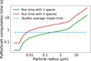 |
Fig. 1 PyMieScatt computation time for the extinction coefficient of a Titan tholin spherical particle vs. the particle size. For each particle size, the Qext are computed on the full wavelength grid of the optical constants (see Sect. 2.1). The green and red lines represent the run time of a model with PYMIESCATT with one and four cloud species, respectively. The time displayed are the median times for ten iterations to avoid outliers. The dashed blue line is the average model time for a cloud-free TAUREX forward model with 100 layers (Al-Refaie et al. 2021). |
2.1 Optical constants
To compute the extinction, scattering, and asymmetry coefficients, the complex optical constants of the particles m(λ) are required (see Eq. (1)). These constants are measured experimentally in laboratories using the Kramers-Kroning analysis and the Lorenz oscillator fit method on the reflection spectra of the powdered compound (Jäger et al. 2003). The variations and features of m(λ) create the absorption features of the aerosols (see Fig. 2). To accurately model cloud and haze absorption bands, the optical indexes must therefore be measured with sufficient spectral resolution (Bohren & Huffman 1983; Kitzmann & Heng 2018). in the literature, however, the spectral resolution and wavelength coverage of available optical indexes varies (Jäger et al. 2003; Dorschner et al. 1995; Zeidler et al. 2013; Henning & Mutschke 1997; Palik 1985; Khare et al. 1984). Other studies, for instance Batalha et al. (2025), have adopted a common wavelength grid to interpolate and/or extrapolate optical indexes between 0.3 to 300 microns. They used a grid with a varying resolution from 2.5 to 250, but recommended a resolution of 300 to interpret JWST datasets following Grant et al. (2023).
Changeat et al. (2025a) interpolated the optical indexes at a resolution of 100 for all the aerosols in TAUREX-PYMIESCATT. In many cases, this resolution is well suited for Mie computations and precomputed Qext grids because of the relatively low number of points, which limits computation time and memory cost. In the interval λ ∈ [0.3-50] μm (i.e., the wavelength range of the EXOMOL cross sections), only 517 wavelength points are needed. In some cases, such as MgSiO3, the optical constants need to be interpolated because they are experimentally measured at a spectral resolution lower than 100. In this case, the interpolation, and hence our knowledge of the optical constants, becomes the dominant error factor. For some species with sharp features, such as SiO2 amorph (or SiO, SiO2 α), a higher resolution is needed (and measured): the 100 resolution does not suffice to accurately interpolate the variations of n(λ) and k(λ), as shown in Fig. 2. For a particle of SiO2 amorph with a = 700 nm, an interpolation of n(λ) and k(λ) at resolution 100 induces a relative error of ≈4% in the tip of the Si - O stretch band. While this level of uncertainty does not affect the retrieval outcomes of transit spectroscopy retrievals (see Fig. 5), it is sufficient to significantly bias the retrieval of directly imaged objects (see Fig. A.1). To correct for this bias, we combined the wavelength grid at resolution 100 from Changeat et al. (2025a) with local higher-resolution grids (between 500 and 1000) in a manually selected key wavelength region to produce smooth Qext features. This method only adds between 30 to 100 points to the wavelength grid, depending on the species, and it is much better suited for a retrieval analysis of high information content (see Fig. A.1).
2.2 Radius grid and Qext computations
We followed Mie theory from (Bohren & Huffman 1983). In exo-atmospheric studies, we seek to constrain the cloud particle mass-mixing ratio, vertical extent, and particle radius a. Codes such as TAUREX or PETITRADTRANS often retrieve a as a free parameter from the cloud absorption properties in the spectrum (i.e., scattering slope and aerosol features). Since cloud layers display a distribution of particles rather than singlesized particles, a few evaluations of Qext at different a are needed for each model. Precomputing Qext can save significant computing time. We precomputed Qext for all the relevant species in Table 1. We describe the procedure for the Titan tholin, but the same steps were applied to all molecules. Based on recent studies, aerosol particle sizes in planetary and substellar atmospheres typically range from about 10 nm to 10 μm (Gao et al. 2020; Teinturier et al. 2025). To capture a conservative range of plausible grains, we adopted a ∈ [0.001, 30] μm and computed Qext with PYMIESCATT (Sumlin et al. 2018) for the wavelengths λ ∈ [0.3,50] μm. We chose these wavelength limits to match those of the EXOMOL cross sections as they are intended to be used together in retrievals (Tennyson et al. 2016).
We did not use the same grid spacing in a for all the species. Instead, we adopted the smallest (in hard-drive space) nonuniform grid that ensured a target accuracy for Qext (see Table 1), which is different for each species. We defined the accuracy by the relative error to the exact computation with PyMieScatt and set it to ε = 10−4. The following paragraph describes how the radius grids are built.
We started by computing the largest grid step δa, which provides an accuracy lower than 6 for the maximum (amax = 30 μm) and minimum (amin = 1 nm) radii, for example, in the case of the tholins, δamin = 0.05 nm and δamax = 1 mm. We recall that for each particle radius, the Qext is computed over a wavelength range with λ ∈ [0.3,50] μm. Thus, for at a given radius, the accuracy is in fact a distribution of values: one for each wavelength. We imposed that for each a, the 90 quantile of the accuracy should be inferior to ε. Using these grids steps, we computed the linear coefficient m and b so that the equation δa = m ∙ a + b verified δamin = 0.05 nm and δamax = 1mm for a ∈ [0.001,30] μm. Using this formula for δa, we computed the radius grid  . Then, for each radius a in
  , we computed the accuracy. When the accuracy was superior to ε for a radius afail, we repeated the above procedure between amin and afail. We thus obtained {m1, b1} for a ∈ [amin, afail] and {m2, b2} for a ∈ [afail, amax] and computed the radius grid
  . We repeated the process until accuracy was reached for the full radius range (between one and four times for the species in Table 1).
Using the method described above, we built a grid of Qext for each species. We considered the species shown in Table 1. As an example, for Titan tholins, a grid of 58 000 radius points is necessary to cover 1 nm to 30 μm, and it requires 240 Mb of memory space. In Fig. 3 we show the error introduced by our linearization of the Mie theory in the case of the Titan tholins. Our grid strategy ensures that each radius has more than 90% of the Qext relative error below the accuracy limit of 10−4 (see Fig. 3), which should be indistinguishable in current JWST and Ariel retrievals, but provides significant speed-ups.
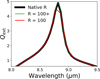 |
Fig. 2 Extinction coefficient for a 700 nm SiO2 amorph particle vs. wavelength. The black, red, and green lines show the Qext computed using optical constants at native resolution, at a resolution of 100, and at a global resolution of 100, respectively, but with a local 500 resolution for key features. |
Aerosol species now available on the Zenodo repository with the respective sizes of the associated grids and reference of the optical indexes.
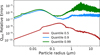 |
Fig. 3 Qext relative error between PYMIESCATT and linear interpolation for each radius interval in the titan tholin grid. For each radius, Qext is computed for 517 wavelengths from 0.3 to 50 microns. The 0.5, 0.9, and 0.99 quantile shown in red, blue, and green, respectively, are computed at each radius from the relative error vs. wavelength array. |
2.3 Scattering coefficient and asymmetry parameter
Although we primarily focused on Qext, Mie theory was also used to compute the scattering efficiency Qscat and asymmetry parameter g. While Qscat and g are not currently included in free atmospheric retrieval frameworks, they are commonly required by self-consistent models. Consequently, eliminating on-the-fly Mie calculations in the general case requires precomputing all three quantities. As Qscat and g are also computed with the Mie coefficients an and bn, PYMIESCATT computes the three coefficients all at once,
 (2)
(2)
and
 (3)
(3)
where α is the scattering angle and p(a, α) is the scattering phase function. We refer to Kitzmann & Heng (2018) for the detailed expression of p(a, α) and to Bohren & Huffman (1983) for the full derivation. Thus, for each of our Qext grids, we also computed one grid for Qscat and another for g. These grids used the same radius grids as for Qext, so we remind users that they might not be as optimal (i.e., we did not impose a tolerance criterion for Qscat and g). Nonetheless, performing the same error analysis as for Qext, we found that the accuracy is similar, with our grid most of the time satisfying our tolerance criterion of ε = 10−4. For Mg2SiO4 amorp sol - gel, MgSiO3 amorph glass, MgSiO3 amorph sol - gel, and the Titan tholins, the relative error on Qscat was superior to 6 for very small particle radii, that is, a < 10 nm. To correct this, we decreased the radius grid step in this region for these four species. When we added only ≈500 more radius steps, the accuracy of the four Qscat grids listed above increased and passed our threshold of ε = 10−4. The Qscat and g grids are also available on Zenodo4 and have the same memory size as their Qext counterparts (see Table 1). However, since TAUREX does not use Qscat and g, we did not test these grids further in the self-retrieval verification process described below.
2.4 Synthetic spectra
Our method ensures relative errors on Qext below 0.1% for all the species. However, radiative transfer is a highly nonlinear process with respect to opacities (their effect is via the Beer Lambert exponential law), even negligible errors in the Qext and linearizations can introduce significant differences in the final spectrum (and retrieved parameters, because the sampled space is also nonlinear). To assess the difference of the TAUREX-PCQ approach for aerosol versus full Mie (i.e., PYMIESCATT) retrievals, we conducted four different tests (see Table 2). We considered standard scenarios in transit and emission spectroscopy by direct imaging with JWST and with the upcoming Ariel Telescope (Tinetti et al. 2021). Each test case we created was strongly inspired by a real exoplanet, but we do not claim here that the simulations we present are relevant for these particular exoplanets. We studied atmospheres similar to those of WASP-107 b, GJ 436 b, HD 189733 b, and 2MASS J2236+4751 b (hereafter 2M2236 b; Dyrek et al. 2024; Changeat et al. 2025a; Mukherjee et al. 2025; Moses et al. 2011; Bowler et al. 2017). To simulate these cases, we used the code TAUREX. The parameters used for the simulations are summarized in Tables B.1 and B.2. For the JWST WASP 107 b synthetic spectra, we used PANDEXO to simulate the error bars (Batalha et al. 2017). We used the uncertainties from the real observations for 2M2236 b since this information is readily available (PID:1188). For Ariel, we employed the radiometric model ArielRad5 to simulate realistic tier 3 noise in the case of GJ 436 b and HD 189733 b (Mugnai et al. 2020). The four simulated observations, obtained after convolving the atmospheric model with the instrument noise profiles, are shown in Fig 4. The retrievals with the best-fit model for the on-the-fly Mie calculation versus our TAUREX-PCQ approach are also shown and discussed in the next section. In every case, the input simulation is scattered using the standard deviation from the noise profiles (i.e., we assumed Gaussian noise and used a single instance).
Overview of the test cases used to validate our approach.
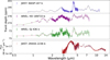 |
Fig. 4 Synthetic spectra created for the self-retrievals, inspired by WASP 107 b, HD 189733 b, GJ436 b, and 2MASS 2236b. To generate the error bars for WASP 107 b, we use the PANDEXO framework (Batalha et al. 2017). The error bars for 2MASS 2236 b come from real JWST observations (PID:1188). For ARIEL, we made use of ARIELRAD to simulate tier 3 noise, stacking two transits for HD 189733 b and ten for GJ436 b. In each panel, the colored lines represent the best-fit models using TAUREX-PyMieScatt and our grid-based methods. |
3 Results
3.1 JWST transmission spectroscopy for WASP 107b
WASP 107 b is a warm (Teff = 740 K) Neptune with an inflated radius of ≈0.84RJ that shows signs of photochemistry, significant mixing, disequilibrium chemistry, and a 10 μm silicate absorption feature. This absorption signature at 10 μm is created by the stretching of Si-O atomic bonds in aerosols. The family of molecules that contributes to this feature (the silicates) regroups among other SiO, SiO2, MgSiO3, Mg2SiO4, or olivine (MgFeSiO4). These particles condense with different crystalline structures, for instance, amorphous or alpha for SiO2, depending on the formation conditions. Different structures of the particles will yield different optical indexes and change the shape of the resonance bands. For WASP 107 b, we chose to simulate the atmosphere using MgSiO3 in its amorphous glass form. The atmospheric parameters used to create the synthetic spectra, summarized in Tables B.1 and B.2, are inspired from Changeat et al. (2025a). We built our synthetic spectrum with TAUREX including error bars from JWST NIRISS, NIR-Spec G395H, and MIRI LRS observation and scattering the data points. The MgSiO3 amorph glass cloud layer has particles with a radius of 0.5 μm. In Fig. 5 we show the posterior distribution of the same retrieval performed with on-the-fly Mie computation and TAUREX-PCQ. The retrieved parameters and posterior distributions between the two methods are the same, which validates our approach for JWST transits of this quality. We recorded the computation time, and the TAUREX-PCQ retrieval was 1.4 times faster than the retrieval using PYMIESCATT.
However, when more species are included, the two methods scale differently. This is because of the a dependence of computation times with PYMIESCATT, which increase with larger a, as described previously, and significantly penalize retrievals with a larger number of species (i.e., sampled a) and live points. With precomputed Qext grids, several cloud species do not significantly change the computational time. When we included four condensed species (i.e., SiO, SiO2, MgSiO3, and Mg2SiO4) in a similar WASP-107 b scenario, the TAUREX-PCQ retrieval was 17 times faster.
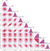 |
Fig. 5 Posterior distributions for WASP 107 b inspired self-retrieval. PYMIESCATT and TAUREX-PCQ are shown in blue and red, respectively. The median value of each retrieved parameter is shown on top of the corresponding histogram. The truth values are displayed in black. |
3.2 Ariel transmission spectroscopy of HD 189733 b and GJ436b
By observing ≈1000 exoplanet atmosphere, the Ariel mission will be able to study clouds and aerosols of exoplanets on a population scale. As a complementary example to the JWST simulations and to highlight the relevance of aerosol modeling with Ariel, we also explored simulations with this future observatory. We chose to simulate two synthetic bright exoplanets inspired by the hot Jupiter HD 189733 b for which SiO26 might be present, and the sub-Neptune GJ436 b, for which aerosols similar to the tholins on Titan might explain the blueward Mie scattering slope. We used atmospheric parameters from Zhang et al. (2024) and Inglis et al. (2024) for HD 189733 b and from Mukherjee et al. (2025) for GJ436b to build our synthetic spectrum with TAUREX (see Tables B.1 and B.2). Then, we used ARIELRAD to simulate the noise for a transit spectrum, assuming that the target is observed in tier 3 resolution (i.e., native Ariel resolution), stacking two and ten transits for HD 189733 b and GJ436 b, respectively (Mugnai et al. 2020). The posterior distributions for both planets are shown in Figs. A.2 and A.3. As for the previous WASP 107 b JWST case, each figure shows the on-the-fly PyMieScatt retrieval versus the TAUREX-PCQ retrieval. As in the JWST case, the retrieved parameters for HD 189733 b and GJ 436 b with Ariel are independent of the aerosol model we used, which validates that our Qext grid approach is numerically converged and equivalent for Ariel data. Similar speed improvements are observed: the TAUREX-PCQ retrieval is 2.3 times faster for HD 189733 b and 2.75 faster for GJ 436 b. For the Ariel survey concept, speed-ups of this order are crucial to ensure the analysis of hundreds of atmospheric spectra. In addition, even though the main silicate absorption feature (at λ ≈ 9-10 μm) is beyond the wavelength range of Ariel (0.6-7.9 μm), if priors on the type of particles can be placed (e.g., via synergy with JWST-MIRI (Changeat et al. 2025b) or using more informative aerosol formation models (Ma et al. 2023), Ariel might be able to inform us on the particle properties (e.g., radius, altitude, and cloud density; see Fig. A.2).
3.3 JWST emission spectroscopy of 2MASS J2236+4751 b
While the field of transiting exoplanets is delivering dozens of high-quality atmospheric spectra, observations of brown dwarfs, planetary mass companions, and exoplanets in direct imaging with JWST have yielded spectra with a much higher resolution (R > 2700) and signal-to-noise ratio (S/N > 100) (Miles et al. 2023; Barrado et al. 2023). Currently, these datasets are numerically the most challenging for atmospheric retrievals. Interpreting datasets with these information content challenges our analysis framework in terms of complexity, model accuracy, and convergence times. In particular, a number of these spectra exhibits clear absorption features from condensate species: for instance, L dwarfs have strong silicate absorption features (Miles et al. 2023; Mollière et al. 2025). For these objects, very few Bayesian atmospheric retrievals have been attempted because robust convergence can only be achieved over several months of computations in HPC facilities. It is essential, however, to characterize the clouds of these objects, particularly in the L/T transition, for understanding the mechanisms that shape the atmosphere of L and T dwarfs. L-type objects are notorious for their silicates absorption features, but it is tedious and time-consuming to determine the specific particles that create this feature (Mollière et al. 2025). A significantly decrease in the computational cost of the cloud model is required to enable more widespread retrieval analyses and to test several aerosol hypotheses in reasonable time frames. We validated the benefits of our PCQ approach on a simulated high-information content spectrum in direct imaging. We created a synthetic spectrum inspired by the late-L planetary mass companion 2MASS J2236+4751 b with an added MgSiO3 cloud layer (see specific input parameters in Tables B.1 and B.2; Bowler et al. 2017). We used error bars from observations of the real planet with NIR-Spec IFU and MIRI LRS (PID:1188). The posterior distribution of the retrievals using TAUREX-PYMIESCATT and TAUREX-PCQ are shown in Fig. A.4 and demonstrate that both methods accurately retrieve the appropriate solution. Hence, it is appropriate to use linearized Qext with e < 10−4 for even spectra with the highest information content available today. We note an improvement of 2.1 in the convergence speed for this case.
4 Summary and conclusions
We presented a new approach for incorporating aerosols into atmospheric retrievals that substantially reduces the computational cost of these retrievals. Aerosols are typically modeled by computing extinction, scattering coefficients, and the asymmetry parameter from the complex refractive indices of condensate species by solving the Lorenz-Mie equations for a range of particle radii and wavelengths. However, the repeated evaluation of Mie theory during a free retrieval or self-consistent model is computationally expensive and often dominates the run time. To circumnavigate this bottleneck, we constructed precomputed extinction, scattering, and asymmetry grids for seven aerosol species (silicates and the Titan tholins) covering a wide range of particle radii and wavelengths. This strategy is effectively equivalent to linearizing Mie theory with respect to particle size. We quantified the interpolation errors introduced by this approximation and evaluated their effect on the retrieval performance. In every grid, the 90 quantile of the relative error (i.e., the error on Qext, Qscat, or g) for each particle radius is below 10−4. We also focused on the optical constants, which are required for Mie theory computations. The wavelength resolution that is used for these constants can affect the retrieval outcomes for very high information datasets such as direct imaging. We showed that an adaptive wavelength grid for species with sharp features is required to avoid systematic errors. For the Qext grids, we employed self-retrievals on synthetic spectra based on four representative atmospheric scenarios, each scattered with real or realistic error bars, and we found that the interpolation errors are negligible and do not affect the retrieved atmospheric parameters. When on-the-fly Mie computations were removed, the retrievals converged significantly faster. The speed-up depends on the true particle size and on the number of aerosol species included, with gains of 1.4-2.3 for single-species cases. A key advantage of our method is its scaling with the number of clouds: while the Mie theory approach slows down exponentially as more condensates are added, the TAUREX-PCQ method runtime is essentially independent of the number of clouds. For instance, although a single-cloud retrieval using Qext grids achieved a speed-up of 1.4, the same retrieval with four clouds became 17 times faster than the corresponding retrieval using direct Mie calculations. Most importantly, these significant speed-ups are achieved without any loss in accuracy. This new method for clouds in atmospheric retrieval is essential to enable the retrieval analysis of high-information content datasets within reasonable timescales. Furthermore, it is also a key development to enable the uniform analysis of large exoplanet populations.
Data availability
We make these Qext, Qscat and g grids freely available for the community at https://doi.org/10.5281/zenodo.17456673. We also publish TAUREX-PCQ, publicly available on GitHub at: https://github.com/groningen-exoatmospheres/taurex-PCQ a plugin that integrates the Qext grids in the open source TAUREX3 retrieval framework.
Acknowledgements
M. Voyer acknowledges funding support by CNES. The authors thank P-O. Lagage for his precious inputs and insightful discussions. This project was provided with computing HPC and storage resources by GENCI at TGCC thanks to the grant 2024-15722 and 2025-15722 on the supercomputer Joliot Curie’s SKL and ROME partition. This publication is part of the project “Exoplanet Atmospheres with Next-generation Space Telescopes” with file no. VI.Veni.242.091 (PI: Q. Changeat) of the “NWO Talent Programme Veni Science domain 2024” under the grant https://doi.org/10.61686/QPZSS86131. It is also part of the project “Interpreting exoplanet atmospheres with JWST” with file no. 2024.034 (PI: Q. Changeat) of the research programme “Rekentijd nationale Computersystemen” which is (partly) financed by the Dutch Research Council (NWO) under the grant https://doi.org/10.61686/QXVQT85756. This work used the Dutch national e-infrastructure with the support of the SURF Cooperative using grant no. 2024.034.
References
- Al-Refaie, A. F., Changeat, Q., Waldmann, I. P., & Tinetti, G. 2021, ApJ, 917, 37 [NASA ADS] [CrossRef] [Google Scholar]
- Barrado, D., Mollière, P., Patapis, P., et al. 2023, Nature, 624, 263 [NASA ADS] [CrossRef] [Google Scholar]
- Batalha, N. E., Mandell, A., Pontoppidan, K., et al. 2017, PASP, 129, 064501 [Google Scholar]
- Batalha, N. E., Rooney, C. M., Visscher, C., et al. 2025, Condensation Clouds in Substellar Atmospheres with Virga [Google Scholar]
- Bohren, C. F., & Huffman, D. R. 1983, Absorption and Scattering of Light by Small Particles [Google Scholar]
- Bowler, B. P., Liu, M. C., Mawet, D., et al. 2017, AJ, 153, 18 [Google Scholar]
- Changeat, Q., Bardet, D., Chubb, K., et al. 2025a, A&A, 699, A219 [NASA ADS] [CrossRef] [EDP Sciences] [Google Scholar]
- Changeat, Q., Lagage, P.-O., Tinetti, G., et al. 2025b, On the Synergetic Use of Ariel and JWST for Exoplanet Atmospheric Science [Google Scholar]
- Chubb, K. L., Rocchetto, M., Yurchenko, S. N., et al. 2021, A&A, 646, A21 [NASA ADS] [CrossRef] [EDP Sciences] [Google Scholar]
- Constantinou, S., & Madhusudhan, N. 2024, MNRAS, 530, 3252 [Google Scholar]
- Dorschner, J., Begemann, B., Henning, T., Jaeger, C., & Mutschke, H. 1995, A&A, 300, 503 [Google Scholar]
- Dyrek, A., Min, M., Decin, L., et al. 2024, Nature, 625, 51 [Google Scholar]
- Estrada, B. C., Lewis, D. A., Helling, C., et al. 2025, A&A, 694, A275 [NASA ADS] [CrossRef] [EDP Sciences] [Google Scholar]
- Gandhi, S., de Regt, S., Snellen, I., et al. 2023, ApJ, 957, L36 [NASA ADS] [CrossRef] [Google Scholar]
- Gao, P., Thorngren, D. P., Lee, E. K. H., et al. 2020, Nat. Astron., 4, 951 [NASA ADS] [CrossRef] [Google Scholar]
- Gao, P., Wakeford, H. R., Moran, S. E., & Parmentier, V. 2021, J. Geophys. Res., 126, e2020JE006655 [Google Scholar]
- Grant, D., Lewis, N. K., Wakeford, H. R., et al. 2023, ApJ, 956, L32 [NASA ADS] [CrossRef] [Google Scholar]
- Helling, C. 2019, Annu. Rev. Earth Planet. Sci., 47, 583 [CrossRef] [Google Scholar]
- Helling, C., Samra, D., Lewis, D., et al. 2023, A&A, 671, A122 [NASA ADS] [CrossRef] [EDP Sciences] [Google Scholar]
- Henning, T., & Mutschke, H. 1997, A&A, 327, 743 [NASA ADS] [Google Scholar]
- Huang, H., Ormel, C. W., & Min, M. 2024, A&A, 691, A291 [NASA ADS] [CrossRef] [EDP Sciences] [Google Scholar]
- Inglis, J., Batalha, N. E., Lewis, N. K., et al. 2024, ApJ, 973, L41 [NASA ADS] [CrossRef] [Google Scholar]
- Jäger, C., Dorschner, J., Mutschke, H., Posch, T., & Henning, T. 2003, A&A, 408, 193 [NASA ADS] [CrossRef] [EDP Sciences] [Google Scholar]
- Khare, B. N., Sagan, C., Arakawa, E. T., et al. 1984, Icarus, 60, 127 [CrossRef] [Google Scholar]
- Kiefer, S., Samra, D., Lewis, D. A., et al. 2024, A&A, 690, A244 [NASA ADS] [CrossRef] [EDP Sciences] [Google Scholar]
- Kitzmann, D., & Heng, K. 2018, MNRAS, 475, 94 [NASA ADS] [CrossRef] [Google Scholar]
- Kothari, H., Cushing, M. C., Burningham, B., et al. 2024, ApJ, 971, 121 [NASA ADS] [CrossRef] [Google Scholar]
- Kühnle, H., Patapis, P., Mollière, P., et al. 2025, A&A, 695, A224 [NASA ADS] [CrossRef] [EDP Sciences] [Google Scholar]
- Ma, S., Ito, Y., Al-Refaie, A. F., et al. 2023, ApJ, 957, 104 [NASA ADS] [CrossRef] [Google Scholar]
- Matthews, E. C., Mollière, P., Kühnle, H., et al. 2025, ApJ, 981, L31 [Google Scholar]
- Miles, B. E., Biller, B. A., Patapis, P., et al. 2023, ApJ, 946, L6 [NASA ADS] [CrossRef] [Google Scholar]
- Min, M., Ormel, C. W., Chubb, K., Helling, C., & Kawashima, Y. 2020, A&A, 642, A28 [NASA ADS] [CrossRef] [EDP Sciences] [Google Scholar]
- Mollière, P., Wardenier, J. P., van Boekel, R., et al. 2019, A&A, 627, A67 [Google Scholar]
- Mollière, P., Kühnle, H., Matthews, E. C., et al. 2025, A&A, 703, A79 [NASA ADS] [CrossRef] [EDP Sciences] [Google Scholar]
- Moses, J. I., Visscher, C., Fortney, J. J., et al. 2011, ApJ, 737, 15 [Google Scholar]
- Mugnai, L. V., Pascale, E., Edwards, B., Papageorgiou, A., & Sarkar, S. 2020, Exp. Astron., 50, 303 [NASA ADS] [CrossRef] [Google Scholar]
- Mukherjee, S., Schlawin, E., Bell, T. J., et al. 2025, ApJ, 982, L39 [Google Scholar]
- Mullens, E., Lewis, N. K., & MacDonald, R. J. 2024, ApJ, 977, 105 [Google Scholar]
- Murphy, M. M., Beatty, T. G., Schlawin, E., et al. 2024, Nat. Astron., 8, 1562 [NASA ADS] [CrossRef] [Google Scholar]
- Ohno, K., Okuzumi, S., & Tazaki, R. 2020, ApJ, 891, 131 [Google Scholar]
- Palik, E. D. 1985, Handbook of Optical Constants of Solids [Google Scholar]
- Rigby, J., Perrin, M., McElwain, M., et al. 2023, PASP, 135, 048001 [NASA ADS] [CrossRef] [Google Scholar]
- Sumlin, B. J., Heinson, W. R., & Chakrabarty, R. K. 2018, JQSRT, 205, 127 [NASA ADS] [CrossRef] [Google Scholar]
- Teinturier, L., Charnay, B., Spiga, A., & Bezard, B. 2025, Clouds as the Driver of Variability and Colour Changes in Brown Dwarf Atmospheres [Google Scholar]
- Tennyson, J., Yurchenko, S. N., Al-Refaie, A. F., et al. 2016, J. Mol. Spectrosc., 327, 73 [Google Scholar]
- Tinetti, G., Eccleston, P., Haswell, C., et al. 2021, Ariel: Enabling Planetary Science across Light-Years [Google Scholar]
- Tsai, S.-M., Lee, E. K. H., Powell, D., et al. 2023, Nature, 617, 483 [CrossRef] [Google Scholar]
- Voyer, M., Changeat, Q., Lagage, P.-O., et al. 2025, ApJ, 982, L38 [Google Scholar]
- Zeidler, S., Posch, T., & Mutschke, H. 2013, A&A, 553, A81 [NASA ADS] [CrossRef] [EDP Sciences] [Google Scholar]
- Zhang, M., Paragas, K., Bean, J. L., et al. 2024, AJ, 169, 38 [Google Scholar]
Ariel will observe thousands of exoplanets and produce up to three transmission spectra a day, with wavelengths from 0.7 to 7.8 microns that are sensitive to haze and clouds (Tinetti et al. 2021).
TAUREX-PYMIESCATT is available at https://github.com/groningen-exoatmospheres/taurex-pymiescatt
For reference, Ariel simulations employ: ArielRad v2.4.26, ExoRad v2.1.111, Payload v0.0.17.
We here include the amorphous glass form of MgSiO3.
Appendix A Additional figures
Figure A.1 shows the impact of the resolution of the optical indexes on the retrieved parameters for a 2M 2236 b inspired planet with an added SiO2 α absorption feature. Then, we show the posterior distributions for the HD 189733 b, GJ 436 b and 2M 2236 b inspired self-retrieval respectively in Fig. A.2, Fig. A.3 and Fig. A.4.
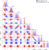 |
Fig. A.1 Posterior distributions for two retrievals on a 2M 2236 b inspired planet with a SiO2 α absorption feature. Truths are shown in black. The blue retrieval uses optical constants at resolution 100 whereas the red retrieval utilize a mix 100 and 1000 resolution for the optical constants. |
Appendix B Additional tables
Tables B.1 and B.2 summarize the atmospheric parameters used to create the synthetic spectra shown in Fig. 4.
Parameter used for generate the synthetic spectra 1/2.
Parameter used for generate the synthetic spectra 2/2.
All Tables
Aerosol species now available on the Zenodo repository with the respective sizes of the associated grids and reference of the optical indexes.
All Figures
|
Fig. 1 PyMieScatt computation time for the extinction coefficient of a Titan tholin spherical particle vs. the particle size. For each particle size, the Qext are computed on the full wavelength grid of the optical constants (see Sect. 2.1). The green and red lines represent the run time of a model with PYMIESCATT with one and four cloud species, respectively. The time displayed are the median times for ten iterations to avoid outliers. The dashed blue line is the average model time for a cloud-free TAUREX forward model with 100 layers (Al-Refaie et al. 2021). |
| In the text | |
|
Fig. 2 Extinction coefficient for a 700 nm SiO2 amorph particle vs. wavelength. The black, red, and green lines show the Qext computed using optical constants at native resolution, at a resolution of 100, and at a global resolution of 100, respectively, but with a local 500 resolution for key features. |
| In the text | |
|
Fig. 3 Qext relative error between PYMIESCATT and linear interpolation for each radius interval in the titan tholin grid. For each radius, Qext is computed for 517 wavelengths from 0.3 to 50 microns. The 0.5, 0.9, and 0.99 quantile shown in red, blue, and green, respectively, are computed at each radius from the relative error vs. wavelength array. |
| In the text | |
|
Fig. 4 Synthetic spectra created for the self-retrievals, inspired by WASP 107 b, HD 189733 b, GJ436 b, and 2MASS 2236b. To generate the error bars for WASP 107 b, we use the PANDEXO framework (Batalha et al. 2017). The error bars for 2MASS 2236 b come from real JWST observations (PID:1188). For ARIEL, we made use of ARIELRAD to simulate tier 3 noise, stacking two transits for HD 189733 b and ten for GJ436 b. In each panel, the colored lines represent the best-fit models using TAUREX-PyMieScatt and our grid-based methods. |
| In the text | |
|
Fig. 5 Posterior distributions for WASP 107 b inspired self-retrieval. PYMIESCATT and TAUREX-PCQ are shown in blue and red, respectively. The median value of each retrieved parameter is shown on top of the corresponding histogram. The truth values are displayed in black. |
| In the text | |
|
Fig. A.1 Posterior distributions for two retrievals on a 2M 2236 b inspired planet with a SiO2 α absorption feature. Truths are shown in black. The blue retrieval uses optical constants at resolution 100 whereas the red retrieval utilize a mix 100 and 1000 resolution for the optical constants. |
| In the text | |
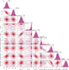 |
Fig. A.2 Same as Fig. 5 but for HD 189733 b. |
| In the text | |
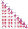 |
Fig. A.3 Same as Fig. 5 but for GJ 436 b. |
| In the text | |
 |
Fig. A.4 Same as Fig. 5 but for 2M 2236 b. |
| In the text | |
Current usage metrics show cumulative count of Article Views (full-text article views including HTML views, PDF and ePub downloads, according to the available data) and Abstracts Views on Vision4Press platform.
Data correspond to usage on the plateform after 2015. The current usage metrics is available 48-96 hours after online publication and is updated daily on week days.
Initial download of the metrics may take a while.