© The Authors 2026

1. Introduction

The making of large-scale magnetism by turbulent fluid flow in symmetry-broken rotating systems, such as stars or galaxies, is known as the large-scale dynamo effect, and is an archetypal case of highly multiscale turbulent dynamics in astrophysics. This problem presents us with major theoretical challenges, starting with its intrinsically three-dimensional nature; we have come to rely increasingly on high-performance computing (HPC) to decipher these challenges. Regular numerical progress has been achieved in modelling the convectively driven solar dynamo (Parker 1955) since the pioneering work of Gilman (1983) (see reviews by Brandenburg & Subramanian 2005; Rincon 2019; Charbonneau 2020; Käpylä 2025 and, over the last ten years, modelling work by Guerrero et al. 2016; Hotta et al. 2016; Käpylä et al. 2017; Strugarek et al. 2018; Hotta & Kusano 2021; Brun et al. 2022; Käpylä 2023; Warnecke et al. 2025). Magnetohydrodynamic (MHD) modelling of the solar cycle nevertheless remains a numerical quagmire; there are discrepancies between models currently attributed to several physical effects, including rotation, magnetic feedbacks, geometry, and to specific numerical implementations (Charbonneau 2020). However, an even more general question looms: turbulence regimes accessible to simulations, notably characterised by the kinetic and magnetic Reynolds numbers, Re and Rm, remain far from the astrophysical realm (bottom right of Fig. 1). Accordingly, we need to understand how far we are from accurate computer models of astrophysical dynamos. Are they even on the horizon ?

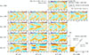Fig. 1. Butterfly diagrams ${\overline{B}}_x(z,t)$ of large-scale non-linear helical dynamo modes vs Re and Rm. Run S01 (Pm = 0.5) is the rightmost plot; run T06 (Pm = 4) of R21 is the topmost plot. The parameter range spanned is shown at the bottom right. The same colour scale is used in all plots.

Addressing these questions requires proceeding methodically towards large Re and Rm, preferably with the right ordering between the two. However, global models, many relying on numerical dissipation, have favoured large-scale realism (spherical geometry, differential rotation, radial stratification) at the expense of turbulent non-linearities and explicit dissipation. While tricks can be used to probe linear large-scale dynamos at large Rm (Tobias & Cattaneo 2013), in minimal controlled set-ups with reduced effective dimensionality, they cannot describe the relevant dynamical non-linear regimes (Pongkitiwanichakul et al. 2016). Overall, limited work has been devoted (in solar physics at least; see e.g. Sheyko et al. (2016), Schaeffer et al. (2017), Aubert et al. (2017) for the faster-rotating geodynamo) to a careful exploration via direct numerical simulation (DNS), using explicit viscosity and resistivity, of the non-linear regime at large Re and Rm. This is an issue for several reasons; for instance, the large-Rm asymptotics of catastrophic quenching of helical dynamos (Brandenburg & Subramanian 2005) cannot be studied with global simulations (Simard et al. 2016). Del Sordo et al. (2013), and more recently Rincon (2021) (hereafter R21) and Brandenburg & Vishniac (2025), have attempted to explore in simpler local cartesian set-ups how non-linear dynamos with hemispheric helicity distributions, such as those expected from rotating convection, change with Re and Rm and, in relation to catastrophic quenching, what dominant magnetic-helicity budget balances are satisfied asymptotically. In addition, most models have magnetic Prandtl numbers Pm > 1, opposite to the Sun. Overall, many uncertainties remain as to how small- and large-scale dynamics couple at large Rm (Warnecke et al. 2025).

This Letter expands significantly on R21 to probe large-scale non-linear helical dynamos at large Re and Rm. I present new analyses that point to an ultimate large-Rm solar dynamo regime involving magnetic helicity fluxes, and compute such numerical solutions at both Pm > 1 and Pm < 1. A standardised comparison with global simulations suggests that they are not in this regime, and I pinpoint their key intrinsic limitations. I also discuss the current limitations of my own results, and possible ways for global models to reach the ultimate regime at reasonable cost.

2. Cartesian helical dynamo simulations

I considered the 3D MHD numerical experiment introduced in R21 (see Appendix A) to study the non-linear phase of a helically driven large-scale turbulent dynamo effect. In a spatially periodic, cartesian box elongated along the z-direction, a turbulent flow was forced at the (x, y) box scale by a Galloway-Proctor-inspired helical forcing term reversing at z = 0 (Galloway & Proctor 1992). Anticipating the large-scale nature of the emerging dynamo mode, the box was made larger by a factor of 4 in the z direction than in the (x, y) directions, L_z/(L_x, L_y) = 4 in order to allow a minimal scale-separation between the turbulence injection scale, L_f ∼ L_x, and the scale ∼L_z of the dynamo mode itself. This forcing and set-up ensures a hemispheric sinusoidal distribution of kinetic helicity reversing at the ‘equator’ (here z = 0, L_z/2, see Fig. B.1), typical of rotating turbulent astrophysical systems, such as solar convection banana cells. The goal, then, is to grasp how the non-linear dynamo properties change with Re = u_rms/(k_fν) and Rm = u_rms/(k_fη). Here, k_f = 2π/L_f is the forcing wavenumber, u_rms is the rms turbulent velocity, ν is the kinematic viscosity, and η is the magnetic diffusivity.

This maximally simplified setting still captures the physical essence of what I think is minimally required to drive a spatially distributed large-scale dynamo in a rotating turbulent system, such as the Sun or a galaxy. The experiment is fully 3D and non-linear, and has built-in scale-separation without the burden of complex geometry and stratification effects. Its turbulence has a realistic order-one correlation to turnover time ratio, with a well-defined hemispheric turbulent helicity distribution, but zero net volume-averaged helicity, a key feature to escape the catastrophic dynamo quenching (see e.g. Brandenburg 2001 and R21). This simplicity enables the use of exponentially fast converging spectral methods to probe large Re and Rm regimes with an optimal use of the numerical resolution and, critically, all dissipative processes under control. Using the incompressible MHD spectral code SNOOPY with 2/3 dealiasing (Lesur & Longaretti 2007) at resolutions up to 512² × 2048, one can reach large Re, Rm = O(3000) by astrophysical MHD standards.

The R21 simulations are complemented by a new high-resolution run, labelled S01, with Re = 2800 and Pm = ν/η = 0.5 (Table B.1), to probe the Pm < 1 behaviour of the dynamo, typical of the solar interior. Instead, the highest-resolution T06 simulation in R21 at Rm = 2800 was focused on pushing into the large-Rm asymptotics, and limited to Pm = 4 to adequately resolve all scales. Each simulation was run for a minimum of 50 forcing times 2π/ω_f (up to ∼200 actual flow turnover times L_f/u_rms) to allow for the statistical emergence, saturation, and long-time evolution of a large-scale dynamo mode. A mosaic overview of butterfly diagrams of the x-component ${\overline{B}}_x(z,t)$ of the (x, y)-averaged magnetic field emerging in the simulations is shown in Fig. 1. In all runs, a large-scale mode is excited and dynamically sustained. Two prominent trends can be seen:

• As Rm (Pm) increases at constant Re, the system bifurcates from a bistable-like steady state to a migrating wave state, and the magnitude of $\overline{B}$ decreases (see Table B.1 and Fig. D.2;).

• At large Rm, the dynamo wave period increases with increasing Re (decreasing Pm); at lower Rm, the system also transitions from a steady state to a wave as Re increases.

The results of the new S01 run (Pm = 0.5) are similar to the larger Rm, lower Re run T06 (Pm = 4). This includes the dynamo wave pattern and large-scale field saturation level (Table B.1). Their time-averaged kinetic and magnetic energy spectra are shown in Fig. B.2. The magnetic and kinetic dissipative cutoffs, k_η = 2π/L_η and k_ν = 2π/L_ν are closer in S01, as expected. However, the factor of eight difference in Pm only has a modest effect on the overall mode and turbulent cascades.

Magnetic helicity is an important near-invariant in this problem (Brandenburg & Subramanian 2005; Moffatt 2016; Kleeorin & Rogachevskii 2022), and a detailed analysis of its dynamics is key to unlocking the complexity of this landscape. Building on R21, I show in Appendix C that the simulations can be divided into three distinct regimes (Fig. C.1): a low-Rm resistive (R) regime up to Rm ∼ 50; an intermediate (I) regime up to Rm = O(500), still subject to a strong small-scale magnetic-helicity quenching bottleneck; and an asymptotic large-Rm ultimate (U) regime where resistive quenching of helicity is asymptotically subdominant at both large and small scales. There, the dominant balance in both large- and small-scale helicity budgets is between electromotive-force-driven helicity generation and the divergences of the z-oriented mean fluxes of helicity, two processes independent of resistivity that non-linearly adjust to each other during the self-consistent dynamical evolution.

This phase diagram illuminates Fig. 1. At low Rm, each hemisphere develops its own steady catastrophically quenched helical dynamo, and there is little communication between the two hemispheres except when Re, and therefore turbulent diffusion becomes significant, thereby triggering weak helicity fluxes in z. The qualitative change in the nature of the solutions at Rm > 50 is therefore interpreted as a symptom of the transition between the low and intermediate regimes. In the ultimate large-Rm regime, on the other hand, magnetic helicity fluxes dominate over resistive dissipation of helicity even at low Re, and are thus freely exchanged between the two hemispheres. This allows the dynamo to escape catastrophic quenching and gives rise to hemispheric synchronicity in the form of migrating α²-dynamo waves, whose period depends on the strength of turbulent diffusion, controlled by Re. Of all runs, only those with Rm > 1000 lie comfortably in the ultimate regime. This includes T05, T06 at Pm ≥ 1, and, importantly, also the new run S01 at Pm < 1.

In Appendix D, I show that a satisfactory diffusive transport model can be devised to fit, and also interpret the simulation results. This model recovers all three regimes with reasonable parameters, such as turbulent magnetic diffusion, fractional helicities, and effective fluctuation and mean-field scales, fitted to the simulation data (Fig. D.1). Most importantly, it correctly predicts the decrease in $\overline{B}$ with Rm in simulations, including the rather sluggish asymptote into the ultimate regime (Fig. D.2).

3. Comparison with global models

Table 1 provides a comparison of the (standardised) parameter regimes of recent spherical global models of the solar dynamo, and of idealised cartesian models of large-scale helical dynamo with spatially reversing helicity distributions: Re, Rm (as defined in this work on forcing wavenumbers), Pm, and $k_{\mathrm{f}}/\overline{k}$ (Appendix D; when k_f was not provided, k_f = ℓ_peak/R_⊙, where ℓ_peak is the peak harmonic of the kinetic energy spectrum, and $\overline{k}=1-2/R_{\odot }$, corresponding to a dipolar or quadrupolar field, were used; *Pm = 1.46 from (Hotta et al. 2016) was used to estimate Rm in Hotta & Kusano (2021). Local DNS models fare much better in terms of Re and Rm, both due to their spectral convergence (for R21 and this work) and to smaller controlled scale separations between the turbulent injection scale and the box scale, which provides more resolution for turbulent dissipative structures. Both Fig. 1 and the analyses in Appendices C–D suggest that most global models are far from the regime touched by T06 and S01. Most lie somewhere in the lower left intermediate-regime quarter of Fig. 1, where the dynamo pattern appears most sensitive to Re and Rm. This may go a long way towards explaining why the outcomes of global simulations, including cycle periods, are extremely model-dependent (Charbonneau 2020), and vary significantly as Pm barely changes at mild Rm (e.g. Käpylä et al. 2017). Our diffusive model, in particular Eqs. (D.11)–(D.13) for $\overline{B}$, further suggests that different fractional helicities injected in convection at different Rossby numbers (encapsulated by the θ parameters of the model) can significantly contribute to the scatter and rotational dependence of global models.

The H-model of Hotta & Kusano (2021) is currently the only global model approaching the turbulent regimes of the T06 and S01 runs. This can be seen by comparing the spectra in their Fig. 4 with Fig. B.2 here. In all cases, the ratio of the peak turbulence injection scale to the magnetic dissipation scale is ∼50. However, there is a subtle but key caveat here. As pointed out by Mitra et al. (2010), and made explicit in Appendix D, the critical Rm_I − U separating the intermediate and ultimate regimes has a strong dependence $\propto {(k_f/\overline{k})}^2$ on the scale-separation between the mean field and turbulent injection scales. In the H-run of Hotta & Kusano (2021), the spectral peak of convection is shifted towards rather small scales (spherical harmonics ℓ ≳ 30) compared to a large-scale spherical dipole or quadrupole, making this scale-ratio ($k_f/\overline{k}\sim 15-30$) much higher than in the present controlled set-up ($k_f/\overline{k}\sim 4-8$; see Table 1 and Appendix D). Because of this large-scale separation inherent to global models (and likely to the Sun itself), I estimate that achieving the ultimate regime with realistic global models may require Rm > 5000. Accordingly, and despite their massive resolution and similar Rm to the present highest-resolution runs, the runs of Hotta & Kusano (2021) likely lie in the core of the intermediate regime, not in the ultimate regime as for S01 and T06. This is further supported by their report (Fig. 3b) of a decrease in $\overline{B}$ with increasing Rm, typical of the intermediate regime (Eq. (D.12) and Fig. D.2). It is also notable in this respect that they find no true oscillating large-scale field in their high-resolution run.

The effective Pm of most global models so far is larger than one, which may be a problem with respect to solar realism. Here, the new results hint at a little piece of good news: the overall similarity between the Pm = 0.5 and Pm = 4 runs suggests that large-scale dynamos with hemispheric helicity distributions, and their saturation at large Rm, may only be weakly dependent on Pm at large Re. Further support for this hypothesis comes from my earlier remark that turbulent helicity fluxes, which are key to the excitation of dynamo waves, should plateau at large Re.

Finally, S01 is above the critical small-scale dynamo (SSD) threshold at Pm = 0.5; considering its similarity with T06 at Pm = 4, this suggests that the issue of SSD–no SSD (Hotta et al. 2016; Hotta & Kusano 2021; Warnecke et al. 2025) may only be secondary to the production of a dynamo with a large-scale component (Kazantsev-model analyses (Malyshkin & Boldyrev 2007, 2009) suggest that the helical dynamo at large Rm is a self-consistent unified multiscale mode like that I simulated, not the mere composition of different modes). The relative vigor of small-scale fields at different Rm and Pm are nevertheless likely to strongly affect the broader turbulent dynamics and how magnetic fields and differential rotation interact. This particular issue cannot be easily examined within my simplified framework.

4. Conclusions and discussion

Using a parameter scan and analysis of maximally simplified three-dimensional cartesian MHD simulations of large-scale non-linear helical dynamos with hemispheric distributions of turbulent kinetic helicity, I have provided detailed numerical evidence and phenomenological arguments for the existence of an asymptotic ultimate non-linear regime of the large-scale solar dynamo involving magnetic helicity fluxes between hemispheres. I obtained corresponding numerical solutions at both Pm > 1 and Pm < 1, and put forward physical interpretations of how the nature of this large-scale dynamo changes in the Re-Rm parameter space. The results, together with the recent study of Brandenburg & Vishniac (2025) with shear and rotation, suggest that these ultimate solutions can currently only be obtained in simplified numerical DNS set-ups where most of the numerical resolution can be put in resolving turbulent structures and transport processes. The large scatter between global solar dynamo simulations outcomes has long been puzzling modellers (Charbonneau 2020). Our analysis highlights that they currently populate a non-asymptotic regime in parameter space where results are highly sensitive to Re and Rm, and likely more generally to the specific implementation of dissipative processes.

Despite the simplifying modelling assumptions required to achieve large Rm, the core physics driving this dynamo (and that of Del Sordo et al. 2013 and Brandenburg & Vishniac 2025 for different flow forcings), is in essence the same as that available in standard global solar dynamo models, in which hemispheric distributions of kinetic helicity have clearly been diagnosed (Simard et al. 2016; Strugarek et al. 2018). Since a generic α²-type mechanism and equally generic turbulent fluxes drive these solutions in the ultimate regime, there is good reason to believe that they bear some relevance to the Sun. However, this simplified approach has its own limitations. Brandenburg & Vishniac (2025) have recently taken on looking at the explicit role of shear and rotation using a similar approach. Their results suggest that the large-scale field does not asymptote towards a small-value in this case. A realistic interplay between the tachocline, differential rotation, and this dynamo is yet to be studied though, and so are the geometric interplay between convection and the Coriolis force to inject helicity, meridional circulation, stratification, and magnetic buoyancy effects, which are all likely to affect the overall picture.

The high resolution and estimated Rm = u_rms/(k_fη) > 5000 required to enter the astrophysically relevant ultimate regime for solar-like scale separations between the mean field and turbulent injection scales are likely to hard-prevent global models with realistic geometries from approaching it in the foreseeable future, at any reasonable computational cost. It would be extremely useful now to produce diagnostics for these simulations, such as those shown in Fig. C.1, to gauge their lack of asymptoticity in Rm. In parallel, it might be possible to tune them into convection regimes with larger injection scales, minimising the scale separation with the desired large-scale field to reach the ultimate regime at lower Rm_I − U. Because magnetic-helicity fluxes play a key role in this regime, they notably provide the strong hemispheric coupling lacking in current global 3D models (Charbonneau 2020). Hence, such a trade-off could produce more reliable solar-like dynamo cycles. Another avenue would be to devise transport closures, for example based on machine-learning informed by the turbulent transport effects isolated here, as such techniques require prior physical insights into the relevant processes to be informative (e.g. Ross et al. 2023; Eyring et al. 2024). Finally, a hydrodynamic anisotropic kinetic alpha effect (AKA/Λ) similar to the large-scale helical MHD dynamo is also possible in helical flows (Frisch et al. 1987). It could be interesting to investigate by similar means whether an ultimate large-Re regime exists for this effect, and how current helicity feeds back, in the saturated regime, on the helical flow driving the dynamo.

Much remains to be done to understand how the essence of the ultimate regime distilled here and in Brandenburg & Vishniac (2025) translates to global models. Judging by the pace at which the size of simulations has increased in recent years, my concern is that this may require a full power plant, something we should be wary of avoiding in the current environmental emergency.

Acknowledgments

This work was granted access to the HPC resources of IDRIS under GENCI allocation 2020-A0080411406, and of CALMIP under allocation P09112. 2.5 MCPU hours were used, for an estimated 8.75 CO2eq tons carbon footprint, using typical 2020 French supercomputer emission numbers (Berthoud et al. 2020). This article is dedicated to my close friend and colleague, Nuno F. Loureiro, who tragically passed away in December 2025.

References

Appendix A: Magnetohydrodynamic model

The code solves the equations of incompressible non-linear magnetohydrodynamics, namely the momentum (Navier-Stokes) equation

$$\begin{array}{c}\hfill \frac{\partial \mathbf{u}}{\partial t}+\mathbf{u}·\mathbf{\nabla }\mathbf{u}=-\mathbf{\nabla }\mathrm{\Pi }+\mathbf{B}·\mathbf{\nabla }\mathbf{B}+\nu \mathrm{\Delta }\mathbf{u}+\mathbf{f}(\mathbf{x},t),\end{array}$$(A.1)

and the induction equation

$$\begin{array}{c}\hfill \frac{\partial \mathbf{B}}{\partial t}+\mathbf{u}·\mathbf{\nabla }\mathbf{B}=\mathbf{B}·\mathbf{\nabla }\mathbf{u}+\eta \mathrm{\Delta }\mathbf{B},\end{array}$$(A.2)

supplemented with

$$\begin{array}{c}\hfill \mathbf{\nabla }·\mathbf{u}=0,\mathbf{\nabla }·\mathbf{B}=0.\end{array}$$(A.3)

Here u and B are the velocity and magnetic fields respectively (there is no mean flow, so a lower case variable is used for the former), B is expressed as an Alfen velocity, Π = P + B²/2 is the total pressure and, as in R21, the forcing term is defined as

$$\begin{array}{c}\hfill \begin{array}{c}\mathbf{f}(\mathbf{x},t)=k_f{A}_f\times \hfill \\ \left(\begin{array}{c}{\displaystyle -2sin(\frac{2\pi y}{L_f}+sin{\omega }_{f}t)sin\frac{2\pi z}{L_z}}\\ {\displaystyle -2cos(\frac{2\pi x}{L_f}+cos{\omega }_{f}t)sin\frac{2\pi z}{L_z}}\\ {\displaystyle sin(\frac{2\pi x}{L_f}+cos{\omega }_{f}t)+cos(\frac{2\pi y}{L_f}+sin{\omega }_{f}t)}\end{array}\right),\hfill \end{array}\end{array}$$(A.4)

where ω_f and A_f are a forcing frequency and amplitude, L_x = L_y ≡ L_f and k_f = 2π/L_f is the forcing wavenumber (L_f = 1, L_z = 4L_f, ω_f = 1 and A_f = 0.1 in all simulations).

Appendix B: Simulation runs

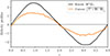Fig. B.1. Time-averaged and (x, y)-averaged kinetic and current helicity z-profiles in run S01 (Rm ≃ 1400, Re ≃ 2900).

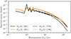Fig. B.2. Energy spectra for run S01 (Rm ≃ 1450, Re ≃ 2900, full line) and run T06 (Rm ≃ 2800, Re ≃ 700, dashed line).

Appendix C: Three regimes

As in R21, I start with the magnetic-helicity budget

$$\begin{array}{c}\hfill \frac{\partial }{\partial t}(\mathbf{A}·\mathbf{B})+\mathbf{\nabla }·{\mathbf{F}}_{{\mathcal{H}}_{\mathbf{m}}}=-2\eta \mathbf{J}·\mathbf{B},\end{array}$$(C.1)

where F_ℋm = c(φB+E×A) is the magnetic-helicity flux, c is the speed of light, E is the electric field, φ is the electrostatic potential, A is the magnetic vector potential, and J = ∇×B is the electric current (in all that follows, I work in the Coulomb gauge). Decomposing B into its mean (average over the (x, y) plane) and fluctuations, $\mathbf{B}(\mathbf{r},t)=\overline{\mathbf{B}}(z,t)+\mathbf{b}(\mathbf{r},t)$ (and similarly for J and A), Eq. (C.1) is separated into large-scale/mean and small-scale/fluctuating parts,

$$\begin{array}{cc}\hfill \frac{\partial }{\partial t}(\overline{\mathbf{A}}·\overline{\mathbf{B}})+\mathbf{\nabla }·{\overline{\mathbf{F}}}_{{\mathcal{H}}_{m,\mathrm{mean}}}& =2\overline{\mathcal{E}}·\overline{\mathbf{B}}-2\eta \left(\mathbf{\nabla }\times \overline{\mathbf{B}}\right)·\overline{\mathbf{B}},\hfill \end{array}$$(C.2)

$$\begin{array}{cc}\hfill \frac{\partial }{\partial t}(\overline{\mathbf{a}·\mathbf{b}})+\mathbf{\nabla }·{\overline{\mathbf{F}}}_{{\mathcal{H}}_{m,\mathrm{fluct}}}& =-2\overline{\mathcal{E}}·\overline{\mathbf{B}}-2\eta \overline{(\mathbf{\nabla }\times \mathbf{b})·\mathbf{b}},\hfill \end{array}$$(C.3)

where ${\overline{\mathbf{F}}}_{{\mathcal{H}}_{m,\mathrm{mean}}}$ and ${\overline{\mathbf{F}}}_{{\mathcal{H}}_{m,\mathrm{fluct}}}$ denote the mean flux of large and small-scale magnetic helicity respectively (see R21 for their detailed definition). ℰ = u × B is the electromotive force (EMF) for a flow u, and we have used ℰ ⋅ B = 0, so that the EMF itself only redistributes helicity into large and small-scale parts. In a statistically steady non-linear state, Eqs. (C.2)–(C.3) reduce to

$$\begin{array}{c}\hfill \frac{|\langle \mathbf{\nabla }·{\overline{\mathbf{F}}}_{{\mathcal{H}}_{m,\mathrm{fluct}}}\rangle +2\eta \langle \overline{\mathbf{j}·\mathbf{b}}\rangle |}{|\langle \mathbf{\nabla }·{\overline{\mathbf{F}}}_{{\mathcal{H}}_{m,\mathrm{mean}}}\rangle +2\eta \langle \overline{\mathbf{J}}·\overline{\mathbf{B}}\rangle |}=1.\end{array}$$(C.4)

Equation (C.4) gives rises to three distinct regimes, established in R21 and now explicitly tagged here in Fig. C.1:

1. A resistively dominated (R) low-Rm regime, where the dominant balance in both Eqs. (C.2)–(C.3) is between the EMF and resistive terms, so that the resistive terms dominate both the numerator and denominator of Eq. (C.4). The same low-Rm helicity budget dominant balance was previously obtained by Mitra et al. (2010) using a similar, albeit distinct forcing.

2. An intermediate-Rm (I) regime, where the resistive term still balances the EMF in Eq. (C.3), and thefore still dominates the numerator in Eq. (C.4), but the dominant balance in Eq. (C.2) is now between the EMF and helicity flux divergence term, so that the mean flux of large-scale helicity dominates in the denominator of Eq. (C.4). This regime was also found, and first probed by Del Sordo et al. (2013) using a similar, albeit distinct forcing.

3. A large Rm, asymptotic ultimate (U) regime, where the resistive helicity dissipation terms are subdominant in both Eqs. (C.2)–(C.3), and the mean fluxes of small-scale and large-scale helicities consequently dominate the numerator and denominator in Eq. (C.4). This regime was first probed by runs T05-T06 in R21 at Pm > 1, but Fig. C.1 further shows that the new run S01 at Pm = 0.5 and Re = 2900 also lies in this regime, and that its helicity budgets are almost identical to those obtained for run T05 at the same Rm but lower Re.

Let us denote the transition Rm between the R and I regimes as Rm_R − I, and that between the intermediate and ultimate regimes as Rm_I − U. The latter is the likely regime of astrophysical interest, and a key question follows: how are current global solar dynamo simulations positioned with respect to Rm_I − U ? This question can be addressed using a phenomenlogical diffusive flux model, described below in Appendix D.

Appendix D: Diffusive helicity-flux model

To make phenomenological progress on the problem, I follow Brandenburg (2001), Mitra et al. (2010) by devising the folllowing diffusive helicity flux model postulating

$$\begin{array}{ccc}\hfill {\overline{\mathbf{F}}}_{{\mathcal{H}}_{m,\mathrm{mean}}}& \widehat{=}\hfill & \hfill -{\kappa }_t\mathbf{\nabla }(\overline{\mathbf{A}}·\overline{\mathbf{B}}),\\ \hfill {\overline{\mathbf{F}}}_{{\mathcal{H}}_{m,\mathrm{fluct}}}& \widehat{=}\hfill & \hfill -{\kappa }_t\mathbf{\nabla }\left(\overline{\mathbf{a}·\mathbf{b}}\right).\end{array}$$(D.1)

Using a dimensional mixing-length argument, we expect

$$\begin{array}{c}\hfill {\kappa }_t=\xi \frac{u_{\mathrm{rms}}}{3k_f},\end{array}$$(D.2)

where ξ is a numerical prefactor to be determined. An effective two-scale parametrisation is adopted by introducing $\overline{k}$, which stands for the dominant wavenumber of the large-scale magnetic field, and k_eff ≥ k_f, an effective wavenumber of turbulent magnetic fluctuations. Also introducing $\overline{\theta }=\overline{k}\overline{\mathbf{A}}·\overline{\mathbf{B}}/{\overline{B}}^2$ and ${\theta }_{\mathrm{eff}}=k_{\mathrm{eff}}\overline{\mathbf{a}·\mathbf{b}}/\overline{b^2}$, the fractional helicities of the large-scale and fluctuation magnetic field respectively, we can express the different terms in Eq. (C.4) as

$$\begin{array}{ccc}\hfill \mathbf{\nabla }·{\overline{\mathbf{F}}}_{{\mathcal{H}}_{m,\mathrm{mean}}}& \sim \hfill & \hfill \overline{\theta }\xi \frac{u_{\mathrm{rms}}}{3}\frac{\overline{k}}{k_f}{\overline{B}}^2,\\ \hfill \mathbf{\nabla }·{\overline{\mathbf{F}}}_{{\mathcal{H}}_{m,\mathrm{fluct}}}& \sim \hfill & \hfill {\theta }_{\mathrm{eff}}\xi \frac{u_{\mathrm{rms}}}{3}\left(\frac{{\overline{k}}^2}{k_{\mathrm{eff}}{k}_f}\right)\overline{b^2},\end{array}$$(D.3)

$$\begin{array}{ccc}\hfill 2\eta \overline{\mathbf{J}}·\overline{\mathbf{B}}& \sim \hfill & \hfill 2\eta \overline{\theta }\overline{k}{\overline{B}}^2,\\ \hfill 2\eta \overline{\mathbf{j}}·\overline{\mathbf{b}}& \sim \hfill & \hfill 2\eta {\theta }_{\mathrm{eff}}{k}_{\mathrm{eff}}\overline{b^2}.\end{array}$$(D.4)

Equation (C.4) then provides a simple prescription for the saturation level of the large-scale field,

$$\begin{array}{c}\hfill \frac{\langle {\overline{B}}^2\rangle }{\langle \overline{b^2}\rangle }=\left(\frac{{\theta }_{\mathrm{eff}}}{\overline{\theta }}\right)\left(\frac{\overline{k}}{k_{\mathrm{eff}}}\right)\frac{1+R{m}_{2-3}/Rm}{1+R{m}_{1-2}/Rm},\end{array}$$(D.5)

with

$$\begin{array}{cc}\hfill R{m}_{R-I}& =\frac{6}{\xi },\hfill \\ \hfill R{m}_{I-U}& =\frac{6}{\xi }{\left(\frac{k_{\mathrm{eff}}}{\overline{k}}\right)}^2.\hfill \end{array}$$(D.6)

In the low-Rm limit (resistive regime),

$$\begin{array}{c}\hfill \frac{\langle {\overline{B}}^2\rangle }{\langle \overline{b^2}\rangle }=\left(\frac{{\theta }_{\mathrm{eff}}}{\overline{\theta }}\right)\left(\frac{k_{\mathrm{eff}}}{\overline{k}}\right).\end{array}$$(D.7)

In the intermediate-Rm regime,

$$\begin{array}{c}\hfill \frac{\langle {\overline{B}}^2\rangle }{\langle \overline{b^2}\rangle }=\frac{6}{\xi }\left(\frac{{\theta }_{\mathrm{eff}}}{\overline{\theta }}\right)\left(\frac{k_{\mathrm{eff}}}{\overline{k}}\right)\frac{1}{\mathit{Rm}}.\end{array}$$(D.8)

Finally, in the large-Rm limit (ultimate regime),

$$\begin{array}{c}\hfill \frac{\langle {\overline{B}}^2\rangle }{\langle \overline{b^2}\rangle }=\left(\frac{{\theta }_{\mathrm{eff}}}{\overline{\theta }}\right)\left(\frac{\overline{k}}{k_{\mathrm{eff}}}\right).\end{array}$$(D.9)

We are now finally in a position to calibrate the above model against the suite of simulations. Figure D.1 for run T06 first shows that the diffusion approximation, Eqs. (D.1)–(D.2), works reasonably well to model both fluxes of large and small-scale magnetic helicity in the highest-Rm simulations, giving consistent values ξ ≃ 0.55 − 0.6. This value is also consistent with previous results obtained by Del Sordo et al. (2013) using a different turbulent forcing (ξ here is the same as κ_f/η_t in their Table 2).

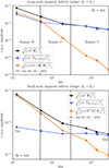Fig. D.1. Helicity budgets for the T and S runs as a function of Rm, with corresponding regime tags and qualitative separations between regimes (vertical dashed lines). The lines and full circles correspond to the T runs (Re ≃ 694 based on T06) in R21; the empty squares show the same quantities for the new Re ≃ 2900, Pm = 0.5 run S01.

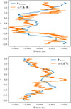Fig. D.2. Turbulent fluxes of large and small-scale magnetic helicity in the T06 run at Rm = 2800, and their respective diffusive fits. The best fit for the turbulent flux of large-scale helicity gives κt = 0.6 urms/(3 kf), and that for the flux or small-scale helicity κt = 0.55 urms/(3 kf).

Figure D.2 shows that this phenomenological effective model can provide a good fit to the results of the simulations, and a sound basis for their interpretation. Two key observations are in order. First, both the model and numerical results suggest a sluggish asymptote of this large-scale dynamo towards the large-Rm limit, that even run T06 at Rm = 2800, corresponding to the rightmost point in the figure, barely starts to trace. Second, as already pointed out by Brandenburg (2001), Mitra et al. (2010) and in the main text, the transition Rm_I − U to the ultimate large-Rm regime scales as the square of the scale separation between the large-scale field and turbulent forcing scale, see Eq. (D.10) with k_eff ∼ k_f. For this set-up, Fig. D.2 shows that Rm_I − U ≃ 670, with $k_{\mathrm{eff}}/\overline{k}=7$ consistent with k_fL_z/(2π) = 4. Were the scale separation between the large-scale dynamo field and turbulent forcing scale significantly larger than that, as expected in global spherical models of the solar dynamo, that transition is expected to occur at much higher Rm_I − U than in the present carefully optimised set-up.

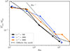Fig. D.3. Comparison of simulations with the diffusive-flux model for $\langle {\overline{B}}^2\rangle /\langle \overline{b^2}\rangle$ as a function of Rm. The model parameters, extracted from fits to the simulations, are ξ ∼ 0.55, $\overline{k}=3$, $k_{\mathrm{eff}}/\overline{k}=7.8$, θeff = 0.15, $\overline{\theta }=0.6$, corresponding to RmR − I = 11 and RmI − U = 670.

All Tables

All Figures

	Fig. 1. Butterfly diagrams ${\overline{B}}_x(z,t)$ of large-scale non-linear helical dynamo modes vs Re and Rm. Run S01 (Pm = 0.5) is the rightmost plot; run T06 (Pm = 4) of R21 is the topmost plot. The parameter range spanned is shown at the bottom right. The same colour scale is used in all plots.
In the text

	Fig. B.1. Time-averaged and (x, y)-averaged kinetic and current helicity z-profiles in run S01 (Rm ≃ 1400, Re ≃ 2900).
In the text

	Fig. B.2. Energy spectra for run S01 (Rm ≃ 1450, Re ≃ 2900, full line) and run T06 (Rm ≃ 2800, Re ≃ 700, dashed line).
In the text

	Fig. D.1. Helicity budgets for the T and S runs as a function of Rm, with corresponding regime tags and qualitative separations between regimes (vertical dashed lines). The lines and full circles correspond to the T runs (Re ≃ 694 based on T06) in R21; the empty squares show the same quantities for the new Re ≃ 2900, Pm = 0.5 run S01.
In the text

	Fig. D.2. Turbulent fluxes of large and small-scale magnetic helicity in the T06 run at Rm = 2800, and their respective diffusive fits. The best fit for the turbulent flux of large-scale helicity gives κt = 0.6 urms/(3 kf), and that for the flux or small-scale helicity κt = 0.55 urms/(3 kf).
In the text

	Fig. D.3. Comparison of simulations with the diffusive-flux model for $\langle {\overline{B}}^2\rangle /\langle \overline{b^2}\rangle$ as a function of Rm. The model parameters, extracted from fits to the simulations, are ξ ∼ 0.55, $\overline{k}=3$, $k_{\mathrm{eff}}/\overline{k}=7.8$, θeff = 0.15, $\overline{\theta }=0.6$, corresponding to RmR − I = 11 and RmI − U = 670.
In the text

References

- Aubert, J., Gastine, T., & Fournier, A. 2017, J. Fluid Mech., 813, 558 [NASA ADS] [CrossRef] [Google Scholar]
- Berthoud, F., Bzeznik, B., Gibelin, N., et al. 2020, hal-02549565v4 [Google Scholar]
- Brandenburg, A. 2001, in Dynamo and Dynamics (Springer), 125 [Google Scholar]
- Brandenburg, A. 2001, ApJ, 550, 824 [Google Scholar]
- Brandenburg, A., & Subramanian, K. 2005, Phys. Rep., 417, 1 [NASA ADS] [CrossRef] [Google Scholar]
- Brandenburg, A., & Vishniac, E. T. 2025, ApJ, 984, 78 [Google Scholar]
- Brun, A. S., Strugarek, A., Noraz, Q., et al. 2022, ApJ, 926, 21 [NASA ADS] [CrossRef] [Google Scholar]
- Charbonneau, P. 2020, Liv. Rev. Solar Phys., 17, 4 [Google Scholar]
- Del Sordo, F., Guerrero, G., & Brandenburg, A. 2013, MNRAS, 429, 1686 [Google Scholar]
- Eyring, V., Collins, W., Gentine, P., et al. 2024, Nat. Climate Change, 14, 916 [Google Scholar]
- Frisch, U., She, Z. S., & Sulem, P. L. 1987, Phys. D, 28, 382 [Google Scholar]
- Galloway, D. J., & Proctor, M. R. E. 1992, Nature, 356, 691 [CrossRef] [Google Scholar]
- Gilman, P. A. 1983, ApJS, 53, 243 [NASA ADS] [CrossRef] [Google Scholar]
- Guerrero, G., Smolarkiewicz, P. K., de Gouveia Dal Pino, E. M., Kosovichev, A. G., & Mansour, N. N. 2016, ApJ, 819, 104 [NASA ADS] [CrossRef] [Google Scholar]
- Hotta, H., & Kusano, K. 2021, Nat. Astron., 5, 1100 [NASA ADS] [CrossRef] [Google Scholar]
- Hotta, H., Rempel, M., & Yokoyama, T. 2016, Science, 351, 1427 [NASA ADS] [CrossRef] [Google Scholar]
- Käpylä, P. J. 2023, A&A, 669, A98 [NASA ADS] [CrossRef] [EDP Sciences] [Google Scholar]
- Käpylä, P. J. 2025, Liv. Rev. Solar Phys., 22, 3 [Google Scholar]
- Käpylä, P. J., Käpylä, M. J., Olspert, N., Warnecke, J., & Brandenburg, A. 2017, A&A, 599, A4 [NASA ADS] [CrossRef] [EDP Sciences] [Google Scholar]
- Kleeorin, N., & Rogachevskii, I. 2022, MNRAS, 515, 5437 [Google Scholar]
- Lesur, G., & Longaretti, P.-Y. 2007, MNRAS, 378, 1471 [NASA ADS] [CrossRef] [Google Scholar]
- Malyshkin, L., & Boldyrev, S. 2007, ApJ, 671, L185 [Google Scholar]
- Malyshkin, L., & Boldyrev, S. 2009, ApJ, 697, 1433 [Google Scholar]
- Mitra, D., Candelaresi, S., Chatterjee, P., Tavakol, R., & Brandenburg, A. 2010, Astron. Nachr., 331, 130 [NASA ADS] [CrossRef] [Google Scholar]
- Moffatt, H. K. 2016, Proc. R. Soc. Lond. Ser. A, 472, 20160183 [Google Scholar]
- Parker, E. N. 1955, ApJ, 122, 293 [Google Scholar]
- Pongkitiwanichakul, P., Nigro, G., Cattaneo, F., & Tobias, S. 2016, ApJ, 825, 23 [Google Scholar]
- Rincon, F. 2019, J. Plasma Phys., 85, 205850401 [NASA ADS] [CrossRef] [Google Scholar]
- Rincon, F. 2021, Phys. Rev. Fluids, 6, L121701 [Google Scholar]
- Ross, A., Li, Z., Perezhogin, P., Fernandez-Granda, C., & Zanna, L. 2023, J. Adv. Model. Earth Syst., 15, e2022MS003258 [Google Scholar]
- Schaeffer, N., Jault, D., Nataf, H., & Fournier, A. 2017, Geophys. J. Int., 211, 1 [NASA ADS] [CrossRef] [Google Scholar]
- Sheyko, A., Finlay, C. C., & Jackson, A. 2016, Nature, 539, 551 [Google Scholar]
- Simard, C., Charbonneau, P., & Dubé, C. 2016, Adv. Space Res., 58, 1522 [NASA ADS] [CrossRef] [Google Scholar]
- Strugarek, A., Beaudoin, P., Charbonneau, P., & Brun, A. S. 2018, ApJ, 863, 35 [Google Scholar]
- Tobias, S. M., & Cattaneo, F. 2013, Nature, 497, 463 [Google Scholar]
- Warnecke, J., Korpi-Lagg, M. J., Rheinhardt, M., Viviani, M., & Prabhu, A. 2025, A&A, 696, A93 [NASA ADS] [CrossRef] [EDP Sciences] [Google Scholar]