| Issue |
A&A
Volume 707, March 2026
|
|
|---|---|---|
| Article Number | A66 | |
| Number of page(s) | 7 | |
| Section | Extragalactic astronomy | |
| DOI | https://doi.org/10.1051/0004-6361/202558667 | |
| Published online | 02 March 2026 | |
One H2 molecule per ten million H atoms reveals sub-parsec-scale cold overdensities at z ∼ 4★
1
Institut d’Astrophysique de Paris, CNRS-SU, UMR 7095 98bis bd Arago 75014 Paris, France
2
Ioffe Institute Polyteknicheskaya 26 194021 Saint-Petersburg, Russia
3
NRC Herzberg Astronomy and Astrophysics Research Centre 5071 West Saanich Road Victoria BC V9E 2E7, Canada
4
Department of Physics and Astronomy, Camosun College 3100 Foul Bay Road Victoria BC V8P 5J2, Canada
5
INAF – Osservatorio Astronomico di Trieste, Via G. B. Tiepolo 11 34143 Trieste, Italy
6
IFPU – Institute for Fundamental Physics of the Universe Via Beirut 2 34151 Trieste, Italy
7
National Institute for Nuclear Physics Via Valerio 2 34127 Trieste, Italy
8
Departamento de Astronomía, Universidad de Chile Casilla 36-D Santiago 7550000, Chile
9
LERMA, Observatoire de Paris, Université PSL, Sorbonne Université 75014 Paris, France
10
Laboratoire de Physique de l’École Normale Supérieure, PSL, CNRS, SU, Université de Paris 75005 Paris, France
11
Centre for Extragalactic Astronomy, Durham University South Road Durham DH1 3LE, UK
★★ Corresponding authors: This email address is being protected from spambots. You need JavaScript enabled to view it.
, This email address is being protected from spambots. You need JavaScript enabled to view it.
Received:
18
December
2025
Accepted:
23
January
2026
Abstract
We present the detection and analysis of H2 absorption at z = 4.24 towards the bright quasar J 0007−5705, which was observed with the Very Large Telescope as part of the ESPRESSO QUasar Absorption Line Survey (EQUALS). The high resolving power of R ≈ 120 000 enables the identification of extremely weak H2 lines in several rotational levels at a total column density of N(H2)≈2 × 1014 cm−2, which is among the lowest ever measured in quasar absorption systems. Remarkably, this constitutes the highest redshift H2 detection to date. Two velocity components are resolved that are separated by only 3 km s−1: a narrow (b ∼ 1.7 km s−1) and a broader (b ≃ 6.2 km s−1) component. Modelling the rotational population of H2 yields a density of log nH/cm−3 ∼ 2.8 and temperature of ∼40 K (typical of the cold neutral medium) for the narrow component and log nH/cm−3 ∼ 1.4, T ∼ 600 K for the warmer, more turbulent component under a moderate ultraviolet (UV) field, suggesting at least a several-megaparsec distance from the quasar. This system reveals the existence of tiny (down to ∼0.01 pc), cold overdensities in the neutral medium. Their detection among only seven damped Lyman-α systems in EQUALS suggests that they may be widespread yet usually remain undetected. H2 provides an exceptionally sensitive probe of these structures: even a minute molecular fraction produces measurable Lyman-Werner absorption lines along the extremely narrow optical beam –the size of the quasar’s accretion disc– when observed at sufficiently high spectral resolution. High-resolution spectroscopy on extremely large telescopes may routinely detect and resolve such structures in the distant Universe, where 21-cm absorption traces the collective contribution of many cold cloudlets towards larger radio background sources.
Key words: ISM: molecules / ISM: structure / quasars: absorption lines
Based on observations collected at the European Southern Observatory under programme ID 112.25NR.
© The Authors 2026
 Open Access article, published by EDP Sciences, under the terms of the Creative Commons Attribution License (https://creativecommons.org/licenses/by/4.0), which permits unrestricted use, distribution, and reproduction in any medium, provided the original work is properly cited.
This article is published in open access under the Subscribe to Open model. This email address is being protected from spambots. You need JavaScript enabled to view it. to support open access publication.
1. Introduction
Molecular hydrogen (H2), the simplest and by far the most abundant molecule in the Universe, plays a central role in tracing the physical conditions of the interstellar and circumgalactic media. Owing to its specific formation, destruction, and excitation processes, it provides sensitive diagnostics of gas density, temperature, and radiation field via its rotational and vibrational populations (e.g. Jura 1975; Bialy et al. 2017). In addition, H2 can reveal dynamical effects such as the dissipation of turbulent energy in vortices and shocks (e.g. Godard et al. 2009; Lesaffre et al. 2020) and phase-transition processes such as condensation and evaporation of cold-neutral-medium (CNM) clouds (Valdivia et al. 2016; Bellomi et al. 2020).
Infrared H2 emission lines are typically detected in dense warm gas illuminated by massive stars (Habart et al. 2003), but they can also arise from diffuse and translucent gas, likely due to the reprocessing of mechanical or ultraviolet (UV) energy (Villa-Vélez et al. 2024). Nevertheless, the most sensitive way to detect H2 remains through electronic (Lyman and Werner) absorption lines against background sources. Since these lines lie in the far-UV, observations of H2 in our Galaxy and up to intermediate redshifts require space-based instruments. Pioneering studies with Copernicus (e.g. Savage et al. 1977) and later with the Far Ultraviolet Spectroscopic Explorer (e.g. Shull et al. 2000; Gillmon et al. 2006) provided a detailed view of molecular gas in the Milky Way and nearby galaxies, while the Cosmic Origins Spectrograph (COS) onboard the Hubble Space Telescope (HST) extended these studies to z ∼ 0.7 (e.g. Muzahid et al. 2015).
At higher redshifts, the Lyman-Werner bands of H2 shift into the optical window accessible from the ground (Levshakov & Varshalovich 1985). In particular, the Ultraviolet and Visual Echelle Spectrograph (UVES) and X-shooter on the Very Large Telescope (VLT) have revealed the presence of H2 in a fraction of damped Lyα systems (DLAs) in quasar spectra at z ∼ 2 − 3 (e.g. Ledoux et al. 2003; Noterdaeme et al. 2008; Balashev et al. 2019). Building on the idea proposed by Stern et al. (2021) that the inner circumgalactic medium in the early Universe may contain a larger neutral fraction than is typically inferred at low redshifts, recent simulations with detailed H I–H2 transition models suggest that such gas can produce DLA-level H I columns while maintaining low molecular fractions (Gurman et al. 2025). This could explain the low detection rate of H2 in most systems at z ∼ 2 − 3, although some sight lines with higher atomic and molecular content likely intersect galactic discs (Ranjan et al. 2018).
Pushing the observations to z ∼ 4 is key to probing the neutral phase, but it introduces additional challenges: the increasing density of the Lyα forest and the dimming of background sources and their declining number all hamper absorption-line studies. Fortunately, the recent discovery of bright quasars at z > 3 (e.g. Boutsia et al. 2020; Wolf et al. 2020) has enabled a high-resolution (R ∼ 120 000) legacy survey of 23 z ∼ 4 quasars with the Echelle SPectrograph for Rocky Exoplanets and Stable Spectroscopic Observations (ESPRESSO, Pepe et al. 2021) on the VLT: the QUasar Absorption Line Survey (EQUALS, Berg et al. 2025).
Here, we report the detection of H2 absorption in a strong DLA at zabs ≈ 4.24 towards J 000736.56−570151.8 (hereafter J 0007−5705; zQ ≈ 4.271). This marks the highest redshift at which H2 absorption has been detected to date. Although only slightly beyond the zabs = 4.22 absorber reported by Ledoux et al. (2006), its much lower column density would likely have remained undetected without the sensitivity and resolution of our observations. These are presented together with the data reduction in Sect. 2. The analysis is described in Sect. 3, and the results are presented in Sect. 4. We discuss the results and conclude in Sect. 5.
2. Observations and data reduction
J 0007−5705 was observed seven times in October 2023, with each observation consisting of a 3053 s on-target ESPRESSO exposure. All exposures were obtained in dark time, and under clear or better conditions with a seeing of < 0.9″ and an airmass of < 1.5; we adopted a 4 × 2 binning in SINGLEHR mode. We reduced the data using ESO ESPRESSO pipeline v3.3.10. Individual exposures were shifted to the barycentric frame and combined into a single 1D spectrum using Astrocook (Cupani et al. 2020). Atmospheric H2O and O2 absorption was modelled in each individual observed exposure using Molecfit (Smette et al. 2015), and the resulting transmission spectra were then combined in the same way as the science data to produce an effective model of the atmospheric transmission in the final spectrum.
3. Analysis
We performed multi-component Voigt profile fitting to derive the column densities (N), redshifts (z), and Doppler parameters (b) of the H I metals and H2 absorption features. Telluric absorption lines were taken into account by including the effective atmospheric transmission in the overall fitted model.
3.1. Neutral hydrogen
We initially reconstructed the unabsorbed quasar continuum using a spline function with nodes placed in absorption-free regions. Over the Ly-α emission line –affected by the DLA– we positioned the spline anchor points manually, guided by a matched quasar composite spectrum. The continuum was then refined by simultaneously fitting the Lyman series lines along with a Chebyshev polynomial. From this procedure, we measured the total neutral hydrogen column density to be  . The effective Doppler parameter and redshift are also well constrained from the sharp edges of the high-order Lyman series to be
  km s−1 and
  (see Fig. 1).
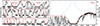 |
Fig. 1. H I Lyman series at z = 4.24 towards J 0007−5705. ESPRESSO data are shown in black, with the synthetic H I profile overplotted in red. For Ly-α, the reconstructed quasar emission profile is indicated by the dashed blue line. |
3.2. Metals
Singly ionised metal absorption lines show that the neutral gas is distributed over only about 50 km s−1 (Fig. 2), with a shallow satellite component separated by about 60 km s−1 from the rest. Atomic data from Morton (2003) were used to fit the metals, except for S II, for which Ritz wavelengths were taken from the NIST Atomic Spectra Database2. A mismatch with the data was evident for S IIλ1253 when using the wavelength from Morton (2003, 1253.805 Å), as noted by Noterdaeme et al. (2007a). In contrast, the Ritz wavelengths provide an excellent match (with 1253.811 Å). While the profiles of O I, Si II and C II are strongly saturated and not fitted, those of S II, Fe II and C II in its first excited level are well reproduced with a seven component model (Table 1).
Results from fitting singly ionised metal lines.
3.3. Molecular hydrogen
H2 absorption lines were detected in the first four rotational levels (see Fig. 2). To account for both continuum uncertainties and frequent blending with intergalactic features, we simultaneously fitted intervening H I components and H2 lines. Two components – one narrow and one broad – were required to model the H2 absorption profile. During the fit, the redshifts (z) and Doppler parameters (b) were tied across rotational levels (J). For the narrow component, the Doppler parameter is primarily constrained by the J = 1 level, which shows numerous transitions spanning from optically thin to intermediate optical depths. In contrast, lines from higher J levels lie mostly in the optically thin regime, where the column densities are largely insensitive to the b value, and the observed line width merely reflects the instrumental line spread function. The broad component is in turn well resolved, and its Doppler parameter is directly constrained by the observed line widths. The optically thin J ≠ 1 lines justify our assumption of a shared b across levels, and, importantly, it allowed us to distinguish between kinematically and thermally distinct components rather than fitting a single, level-dependent effective profile. Allowing b to vary with level may actually cause the contributions of different gas phases to blend, obscuring the underlying structure (see Table 2).
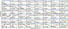 |
Fig. 2. Voigt-profile fit to H2 and metal lines towards J 0007−5705. The origin is set at zH2 = 4.242745. The observed normalised spectrum is shown in black, with the total synthetic absorption in red. H2 components are shown in blue (narrow) and orange (wide) while metal components are shown in green. The transmission from the DLA H I lines, as well as telluric lines (visible in e.g. S IIλ1253 and Fe IIλ1125 panels), is shown in purple. Additional components in grey, fitted jointly with H2 and metal lines, represent intervening Lyman-α forest lines (the v ∼ 20 km s−1 component in the H2W3-0R0 panel is actually Ly-β from a z = 3.838 system, also visible in Ly-α at the blue edge of the Fe IIλ1121 panel). |
Results from fitting H2 lines.
4. Results
4.1. Chemical enrichment
From the total column densities of neutral gas, log N(H I) = 21.36 ± 0.05, and of volatile, singly ionised sulphur, log N(S II) = 14.64 ± 0.02, we inferred the average metallicity of the system to be Z ≃ 0.01 Z⊙ and the depletion of iron to be [Fe/S] = −0.4. One component has stronger depletion with [Fe/S] ≈ −1.2 and coincides (within 0.4 km s−1) with the narrow H2 component. This suggests that the main H2-formation route remains catalytic reactions on the surface of dust grains (e.g. Wakelam et al. 2017), even in this low-metallicity environment (see Glover 2003 for a discussion about the possible dominance of gas-phase reactions in environments with a low dust content).
4.2. Physical conditions
The abundance of H2 in the neutral gas depends on the formation-photodissociation equilibrium (Jura 1975):
 (1)
(1)
with  ; D0 = 5.8 × 10⁻¹¹IUV s−1, where IUV is the UV field intensity in Draine units; 𝒮 is the self-shielding function, which, given the low H2 column density, can be approximated here to unity; and R is the formation rate onto dust grains. When introducing the molecular fraction
  , Eq. (1) becomes
 (2)
(2)
Considering the typical density-to-UV ratio in high-z CNM simulations, 〈n/I/UV〉 = N(H I/1021 cm−2) cm−3 (Gurman et al. 2025), the observed ⟨fH2⟩ ≈ 1.7 × 10⁻⁷ implies an average formation rate of ⟨R⟩ ≃ 2 × 10⁻¹⁸ s−1. This is below the standard CNM value in the local ISM (R ≃ 3 × 10⁻¹⁷ s−1; Jura 1975), but somewhat above expectations at the measured metallicity3. In other words, if average densities from the simulations are assumed, reproducing the H2 constraints requires adopting a formation rate higher than that implied by the mean metal content. This suggests that localised density peaks contribute to H2 production. We note that moderately elevated dust abundances assumptions were also used in the fiducial model of Gurman et al. (2025) to reproduce global H2 detection rates in DLAs.
Next, we investigated the regions where H2 is effectively formed. From the Doppler parameters of the narrow and broad components (b = 1.7 and 6.2 km s−1), assuming pure thermal contribution, it is possible to derive strict upper limits on the gas temperatures to be ∼350 K and ∼4600 K. In other words, the narrow component arises from cold medium, while the broad one could in principle arise from a warmer medium.
Key information about the gas temperature comes from the population of H2 across different rotational levels (Fig. 3). For the narrow component, we measure T01 ≈ 233 ± 33 K, with the distribution across levels (J = 0 − 3) reasonably fitted by a single excitation temperature of Tex ∼ 390 K. While T01 is generally considered a good proxy for the kinetic temperature of the gas in the high-column-density regime, where H2 is self-shielded in the low rotational levels, it more likely represents an upper limit here, since H2 formation tends to overpopulate J = 1 relatively to J = 0. The broad component, in turn, exhibits a flatter excitation diagram with Tex ∼ 600 ± 100 K and a J = 1/J = 0 ratio consistent with 3 –the ratio of statistical weights– i.e., the value expected when the ortho-para ratio is set by H2 formation and destruction processes (Abgrall et al. 1992). This directly indicates that the number density in the broad component is lower than that in the narrow one, where collisional excitation is likely at play. In contrast, in the broad component, the rotational populations do not directly trace the gas kinetic temperature.
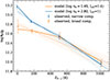 |
Fig. 3. Rotational J = 0 − 3 population of H2 for both components. Points are artificially shifted by ±5 K along the x-axis for clarity. Dashed lines show single-temperature fits (with shaded uncertainties), and solid lines show our best fiducial Cloudy models. |
To further constrain the physical conditions, we investigated the rotational excitation of H2 in constant-density models with Cloudy v25 (see Chatzikos et al. 2023). We assumed a plane-parallel geometry for the two H2-bearing clouds illuminated by a radiation field. As a starting point, we adopted observational constraints whenever possible and standard values when no constraints were available. We included a fixed metagalactic background from Khaire & Srianand (2019) at z = 4.24 and an additional Draine-like UV field, which was treated as a varying parameter. H-ionising photons were removed, as our focus is on the neutral gas. We adopted a Galactic cosmic-ray (CR) ionisation rate of 2 × 10⁻¹⁶ s−1 per H0 (Indriolo et al. 2007) and scaled the metal and dust abundances to 1% the local ISM values, according to the mean DLA metallicity.
Under these assumptions, we created model grids varying only the gas density and the strength of the UV field. Our fiducial model best reproduces the observed H2 excitation in both components for densities of log nH ≈ 2.8 and 1.4 for the narrow and broad components, respectively, under a UV field comparable with the Galactic level for both components (see Figs. 3 and 4). The modelled gas temperatures, 40 and 560 K, correspond to similar thermal pressure (Pth/kB ∼ 2 × 10⁴ K cm−3) in the two components and are consistent with the limits implied by the Doppler parameters. Although we did not attempt to reproduce the metal column densities (as the association between metals and H2 components is uncertain and the depletion pattern is not well constrained), the predicted Si II and C II* columns are reasonably close to (below) the observed values, providing additional confidence in the model.
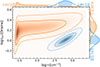 |
Fig. 4. Posterior distributions of the UV field and number density in the broad (orange) and narrow (blue) components. The likelihood was derived by comparing the observed H2J = 0 to J = 3 column densities with those from a grid of Cloudy models and converted into 2D posterior distribution assuming independent flat priors in logarithmic space. The 1D marginalised posteriors are shown along the top and right axes. |
We also tested models with CR ionisation rates varied by a factor of ten and with either baseline or tenfold-higher metal and grain abundances. These provide poorer fits to the H2 excitation and metal column densities, especially when assuming identical UV field and CR rates for both components. A more realistic model, where the cold component has a higher gas-phase metallicity – consistent with stronger iron depletion – but still a low grain abundance (as dust scales sub-linearly with metals), improves the match to the C II* and Si II columns without changing the derived density or UV field. Since C II* excitation scales as nT0.35 (Balashev et al. 2022), the derived temperatures and densities imply a C II*/C II ratio about four times higher in the narrow component, in agreement with the observations.
4.3. Length scales
The inferred densities imply length scales of L ≃ 0.01 pc (narrow H2 component) to a few parsecs (broad component), pointing to a highly fragmented neutral medium, consistent with lower-redshift studies of self-shielded H2 systems (e.g. Jorgenson et al. 2009; Balashev et al. 2011). Here, H2 is merely a tracer of cold gas, yet it reveals that the latter is structured down to very small scales. The fact that the larger cloud is also the more turbulent one is consistent with the trend expected from Larson’s scaling (bturb ∝ L0.38, Larson 1981), providing a self-consistent link between cloud sizes and the underlying turbulent dynamics of the gas. The coexistence of these narrow and broad H2 components likely reflects the underlying nH distribution shaped by turbulence and self-gravity. Such a close physical association could also explain the previously reported increase in the b parameter when the absorption is considered as a whole (e.g. Jenkins & Peimbert 1997; Noterdaeme et al. 2007a; Tchernyshyov 2022).
Motivated by the very small inferred size of the cold cloud, we investigated the possibility of partial coverage. This occurs when the absorbing cloud does not fully cover the background source, which is expected when the cloud’s characteristic size is smaller than, or comparable to, that of the emitter at the absorption wavelength. This effect is most readily identified through a non-zero residual flux at the bottom of saturated lines, as observed, for example, in strong H2 absorption against the parsec-scale broad emission-line regions of quasars (e.g. Balashev et al. 2011).
In the present case, the 0.01-pc length scale inferred for the cold component is comparable to the light-day scale of quasar accretion discs (e.g. Yu et al. 2020), against which the H2 absorption is observed. However, the H2 lines are optically thin, so any partial-coverage signature is expected to be subtle. Nevertheless, introducing the covering fraction as a free parameter for the narrow H2 component yields a covering factor of Cf ∼ 60% and a slight improvement in the fit, most noticeably for a few H2 lines (Fig. 5). This provides an independent, transverse indication of the small cloud size. While the formal preference of the model with partial covering factor is high (ΔAIC ≈ 45, where AIC is the Akaike information criterion), the improvement is modest in a visual sense4. Higher signal-to-noise (S/N) data will be required to robustly confirm partial coverage and to fully disentangle it from possible modelling systematics that could arise from component decomposition, line spread function, local continuum placement, or local deviation in noise properties.
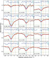 |
Fig. 5. Comparison of best-fit model including partial coverage for the narrow component (red) and assuming full coverage (violet). Only a subset of H2 lines is shown, focusing on transitions where profile differences are most pronounced. Graphical elements follow Fig. 2. The horizontal dashed green line depicts (1 − Cf), the fraction of the background source uncovered by the narrow H2 component. |
In this scenario, the inferred column densities in all rotational levels increase by ≈0.3 dex (Table 3), with no noticeable impact on the derived physical conditions. The inferred cloud size becomes about twice as large, and the predicted metal column densities increase accordingly, bringing them closer to the observed values.
Results from fitting H2 lines allowing for partial coverage for the narrow component.
5. Discussions and conclusion
As the inferred incident UV radiation field is close to the Galactic value (IUV ≃ 1), the absorber likely lies far from the quasar influence. Given the quasar’s brightness (i = 17.2) and redshift (z ≃ 4.27), its UV luminosity (Lν ∼ 3 × 1032 erg s−1 Hz−1) would produce a Galactic-level field only beyond ∼2 Mpc, which is consistent with the ∼1500 km s−1 velocity offset between the quasar and the DLA (∼3 Mpc for pure Hubble flow). This illustrates that proximity in velocity space does not necessarily imply physical proximity. Conversely, the inferred UV field can be explained by the quasar alone, without requiring additional sources. This, in turn, suggests that the absorbing gas may reside far away from any luminous galaxy.
The physical conditions inferred for the H2-bearing gas are broadly consistent with those reported for other H2-bearing DLAs (e.g. Petitjean et al. 2000; Cui et al. 2005; Noterdaeme et al. 2007b; Jorgenson et al. 2010; Albornoz Vásquez et al. 2014; Noterdaeme et al. 2017; Balashev et al. 2019; Klimenko & Balashev 2020; Balashev & Kosenko 2024), as well as for diffuse molecular gas observed along high-latitude lines of sight through the Milky Way disc and halo (Richter et al. 2003; Gillmon et al. 2006; Wakker 2006). However, the gas densities inferred here – particularly for the narrow component – lie towards the upper end of the range typically reported in previous studies. This relatively high density allows trace amounts of H2 to form in a low-metallicity environment without self-shielding. In this optically thin regime, the gas density determines both the kinetic temperature and the H2 excitation. By contrast, the broader component has a density closer to those commonly inferred in the literature, although such densities are usually associated with much higher molecular columns; its temperature is also substantially higher. What distinguishes the present system, therefore, is not extreme physical conditions per se, but the presence of dense, although almost fully atomic, gas.
Even in the cold clump, the molecular fraction remains indeed diminute (log fH2 < −5), highlighting H2 as a sensitive overdensity tracer in low-metallicity neutral gas. Here, it could trace a very compact structure, with a density of log nH ∼ 2.8 over a length scale of only ∼0.01 pc. Yet, the detection of such an absorber among only seven DLAs in the EQUALS sample suggests that these overdensities may be relatively common. This system also likely reflects key evolutionary effects: a higher average gas density at these redshifts and a lower metallicity. The latter reshapes the thermal balance, restricting the formation of cold gas to higher densities because of the reduced metal-line cooling.
A second example is found at z = 2.97 in the EQUALS spectrum of J 0204−3251 (Appendix A). Despite its lower S/N and more uncertain measurements, this system presents similar properties: a relatively low H2 column density distributed over two closely spaced components and a broader component (b ∼ 2.6 km s−1) more highly excited than the narrow one (b ∼ 0.8 km s−1). Cold overdensities could thus actually be frequent enough in the neutral medium at high redshift to collectively build a significant covering fraction.
Individual CNM cloudlets would likely remain undetectable in 21-cm absorption, even with the Square Kilometer Array, because their physical sizes are much smaller than the extent of radio sources. A sufficiently large covering factor could in principle make their collective 21-cm imprint detectable, despite their low volume-filling factor, but the signal could remain shallow, as clouds may spread over a relatively broad velocity interval. In the optical, such compact structures are also challenging to identify at lower spectral resolution or S/N than those achieved here. Their detection in this system was only possible thanks to the achieved resolving power combined with the brightness of the background quasar. Even the broader ∼4-pc component would have remained hidden without the narrow feature flagging the presence of cold gas. ESPRESSO’s sensitivity to narrow absorption lines thus provides a rare probe of the small-scale density structure of the neutral medium at high redshift. Looking ahead, using weak H2 as a routine tracer of CNM cloudlets in low metallicity gas at high redshift (potentially leading to star formation before reaching high molecular fraction; Krumholz 2012; Glover & Clark 2012) will require much larger collecting areas, which will be provided by ANDES on the ELT. Re-observing known H2-bearing systems at higher spectral resolution will also help isolate multi-phase structures and uncover weak H2 components that are otherwise difficult to detect.
Acknowledgments
We thank the referee for useful comments and suggestions. We thank IFPU in Trieste for hospitality. SL acknowledges support by FONDECYT grant 1231187.
References
- Abgrall, H., Le Bourlot, J., Pineau Des Forets, G., et al. 1992, A&A, 253, 525 [Google Scholar]
- Albornoz Vásquez, D., Rahmani, H., Noterdaeme, P., et al. 2014, A&A, 562, A88 [NASA ADS] [CrossRef] [EDP Sciences] [Google Scholar]
- Balashev, S. A., & Kosenko, D. N. 2024, MNRAS, 527, 12109 [Google Scholar]
- Balashev, S. A., Petitjean, P., Ivanchik, A. V., et al. 2011, MNRAS, 418, 357 [Google Scholar]
- Balashev, S. A., Klimenko, V. V., Noterdaeme, P., et al. 2019, MNRAS, 490, 2668 [NASA ADS] [CrossRef] [Google Scholar]
- Balashev, S. A., Telikova, K. N., & Noterdaeme, P. 2022, MNRAS, 509, L26 [Google Scholar]
- Bellomi, E., Godard, B., Hennebelle, P., et al. 2020, A&A, 643, A36 [NASA ADS] [CrossRef] [EDP Sciences] [Google Scholar]
- Berg, T., D’Odorico, V., Boera, E., et al. 2025, The Messenger, 195, 23 [Google Scholar]
- Bialy, S., Burkhart, B., & Sternberg, A. 2017, ApJ, 843, 92 [NASA ADS] [CrossRef] [Google Scholar]
- Boutsia, K., Grazian, A., Calderone, G., et al. 2020, ApJS, 250, 26 [NASA ADS] [CrossRef] [Google Scholar]
- Chatzikos, M., Bianchi, S., Camilloni, F., et al. 2023, Rev. Mexicana Astron. Astrofis., 59, 327 [Google Scholar]
- Cuellar, R., Noterdaeme, P., Balashev, S., et al. 2025, A&A, 694, A294 [NASA ADS] [CrossRef] [EDP Sciences] [Google Scholar]
- Cui, J., Bechtold, J., Ge, J., & Meyer, D. M. 2005, ApJ, 633, 649 [Google Scholar]
- Cupani, G., D’Odorico, V., Cristiani, S., et al. 2020, SPIE Conf. Ser., 11452, 114521U [NASA ADS] [Google Scholar]
- Gillmon, K., Shull, J. M., Tumlinson, J., & Danforth, C. 2006, ApJ, 636, 891 [NASA ADS] [CrossRef] [Google Scholar]
- Glover, S. C. O. 2003, ApJ, 584, 331 [NASA ADS] [CrossRef] [Google Scholar]
- Glover, S. C. O., & Clark, P. C. 2012, MNRAS, 421, 9 [NASA ADS] [Google Scholar]
- Godard, B., Falgarone, E., & Pineau Des Forêts, G. 2009, A&A, 495, 847 [NASA ADS] [CrossRef] [EDP Sciences] [Google Scholar]
- Gurman, A., Sternberg, A., Bialy, S., Cochrane, R. K., & Stern, J. 2025, ApJ, 995, 116 [Google Scholar]
- Habart, E., Boulanger, F., Verstraete, L., et al. 2003, A&A, 397, 623 [NASA ADS] [CrossRef] [EDP Sciences] [Google Scholar]
- Indriolo, N., Geballe, T. R., Oka, T., & McCall, B. J. 2007, ApJ, 671, 1736 [NASA ADS] [CrossRef] [Google Scholar]
- Jenkins, E. B., & Peimbert, A. 1997, ApJ, 477, 265 [NASA ADS] [CrossRef] [Google Scholar]
- Jorgenson, R. A., Wolfe, A. M., Prochaska, J. X., & Carswell, R. F. 2009, ApJ, 704, 247 [Google Scholar]
- Jorgenson, R. A., Wolfe, A. M., & Prochaska, J. X. 2010, ApJ, 722, 460 [NASA ADS] [CrossRef] [Google Scholar]
- Jura, M. 1975, ApJ, 197, 575 [NASA ADS] [CrossRef] [Google Scholar]
- Khaire, V., & Srianand, R. 2019, MNRAS, 484, 4174 [NASA ADS] [CrossRef] [Google Scholar]
- Klimenko, V. V., & Balashev, S. A. 2020, MNRAS, 498, 1531 [CrossRef] [Google Scholar]
- Krumholz, M. R. 2012, ApJ, 759, 9 [NASA ADS] [CrossRef] [Google Scholar]
- Larson, R. B. 1981, MNRAS, 194, 809 [Google Scholar]
- Ledoux, C., Petitjean, P., & Srianand, R. 2003, MNRAS, 346, 209 [NASA ADS] [CrossRef] [Google Scholar]
- Ledoux, C., Petitjean, P., & Srianand, R. 2006, ApJ, 640, L25 [NASA ADS] [CrossRef] [Google Scholar]
- Lesaffre, P., Todorov, P., Levrier, F., et al. 2020, MNRAS, 495, 816 [NASA ADS] [CrossRef] [Google Scholar]
- Levshakov, S. A., & Varshalovich, D. A. 1985, MNRAS, 212, 517 [NASA ADS] [Google Scholar]
- Morton, D. C. 2003, ApJS, 149, 205 [Google Scholar]
- Muzahid, S., Srianand, R., & Charlton, J. 2015, MNRAS, 448, 2840 [Google Scholar]
- Noterdaeme, P., Ledoux, C., Petitjean, P., et al. 2007a, A&A, 474, 393 [NASA ADS] [CrossRef] [EDP Sciences] [Google Scholar]
- Noterdaeme, P., Petitjean, P., Srianand, R., Ledoux, C., & Le Petit, F. 2007b, A&A, 469, 425 [NASA ADS] [CrossRef] [EDP Sciences] [Google Scholar]
- Noterdaeme, P., Ledoux, C., Petitjean, P., & Srianand, R. 2008, A&A, 481, 327 [NASA ADS] [CrossRef] [EDP Sciences] [Google Scholar]
- Noterdaeme, P., Krogager, J.-K., Balashev, S., et al. 2017, A&A, 597, A82 [NASA ADS] [CrossRef] [EDP Sciences] [Google Scholar]
- Pepe, F., Cristiani, S., Rebolo, R., et al. 2021, A&A, 645, A96 [NASA ADS] [CrossRef] [EDP Sciences] [Google Scholar]
- Petitjean, P., Srianand, R., & Ledoux, C. 2000, A&A, 364, L26 [NASA ADS] [Google Scholar]
- Ranjan, A., Noterdaeme, P., Krogager, J. K., et al. 2018, A&A, 618, A184 [NASA ADS] [CrossRef] [EDP Sciences] [Google Scholar]
- Richter, P., Wakker, B. P., Savage, B. D., & Sembach, K. R. 2003, ApJ, 586, 230 [Google Scholar]
- Roman-Duval, J., Jenkins, E. B., Tchernyshyov, K., et al. 2022, ApJ, 935, 105 [Google Scholar]
- Savage, B. D., Bohlin, R. C., Drake, J. F., & Budich, W. 1977, ApJ, 216, 291 [NASA ADS] [CrossRef] [Google Scholar]
- Shull, J. M., Tumlinson, J., Jenkins, E. B., et al. 2000, ApJ, 538, L73 [NASA ADS] [CrossRef] [Google Scholar]
- Smette, A., Sana, H., Noll, S., et al. 2015, A&A, 576, A77 [NASA ADS] [CrossRef] [EDP Sciences] [Google Scholar]
- Stern, J., Sternberg, A., Faucher-Giguère, C.-A., et al. 2021, MNRAS, 507, 2869 [NASA ADS] [CrossRef] [Google Scholar]
- Tchernyshyov, K. 2022, ApJ, 931, 78 [Google Scholar]
- Valdivia, V., Hennebelle, P., Gérin, M., & Lesaffre, P. 2016, A&A, 587, A76 [NASA ADS] [CrossRef] [EDP Sciences] [Google Scholar]
- Villa-Vélez, J. A., Godard, B., Guillard, P., & Pineau des Forêts, G. 2024, A&A, 688, A96 [NASA ADS] [CrossRef] [EDP Sciences] [Google Scholar]
- Wakelam, V., Bron, E., Cazaux, S., et al. 2017, Mol. Astrophys., 9, 1 [Google Scholar]
- Wakker, B. P. 2006, ApJS, 163, 282 [Google Scholar]
- Wolf, C., Hon, W. J., Bian, F., et al. 2020, MNRAS, 491, 1970 [NASA ADS] [CrossRef] [Google Scholar]
- Yu, Z., Martini, P., Davis, T. M., et al. 2020, ApJS, 246, 16 [Google Scholar]
zQ = 4.26 was originally derived from the shallow Si IV and C IV emission in the Irénée du Pont telescope discovery spectrum. The presence of N V absorption at z ≈ 4.27 suggests a redshift at or slightly above this value (see Cuellar et al. 2025).
R < 0.4 × 10⁻¹⁸ s−1, accounting for the sub-linear scaling of R with metallicity (e.g. Roman-Duval et al. 2022) and its  -dependence.
We checked that it is not only driven by the strongest transition, W1-0Q1; see Fig. 5.
Appendix A: H2 at z ∼ 3 towards J 0204-3251
The quasar J 0204-3251 (zQ ≃ 3.8) has also been observed with ESPRESSO as part of the EQUALS survey. It features a strong intervening DLA at zabs ≃ 2.97 with log N(H I) = 21.41 ± 0.01. The metal-line profile is complex, with numerous components spanning ∼250 km s−1, and indicates an overall metallicity of [Si/H] ≈ −0.86 (Fig. A.1). Because silicon is mildly depleted, this value likely represents a lower limit to the true metallicity; Zn II lines are not covered and S II lines fall within the Lyα forest.
Although this spectrum has a lower S/N (particularly in the blue) and covers fewer H2 bands than the main system discussed in this paper, the higher H2 column density enabled the detection of two closely spaced components (Δv ≈ 2.8 km s−1) from J = 0 to J = 3 (Fig. A.2 and Table A.1). The corresponding excitation diagram is shown in Fig. A.3.
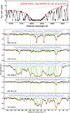 |
Fig. A.1. Fit to H I Ly-α and low-ionisation metals lines in the z = 2.97 DLA system towards J 0204-3251. The zero of the velocity scale corresponds to the strongest H2 component. Colours are as per Fig. 2. |
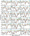 |
Fig. A.2. H2 absorption lines towards J 0204−3251. |
Results from fitting H2 lines towards J 0204−3251.
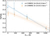 |
Fig. A.3. H2 excitation diagram at z = 2.97 towards J 0204−3251. |
All Tables
Results from fitting H2 lines allowing for partial coverage for the narrow component.
All Figures
|
Fig. 1. H I Lyman series at z = 4.24 towards J 0007−5705. ESPRESSO data are shown in black, with the synthetic H I profile overplotted in red. For Ly-α, the reconstructed quasar emission profile is indicated by the dashed blue line. |
| In the text | |
|
Fig. 2. Voigt-profile fit to H2 and metal lines towards J 0007−5705. The origin is set at zH2 = 4.242745. The observed normalised spectrum is shown in black, with the total synthetic absorption in red. H2 components are shown in blue (narrow) and orange (wide) while metal components are shown in green. The transmission from the DLA H I lines, as well as telluric lines (visible in e.g. S IIλ1253 and Fe IIλ1125 panels), is shown in purple. Additional components in grey, fitted jointly with H2 and metal lines, represent intervening Lyman-α forest lines (the v ∼ 20 km s−1 component in the H2W3-0R0 panel is actually Ly-β from a z = 3.838 system, also visible in Ly-α at the blue edge of the Fe IIλ1121 panel). |
| In the text | |
|
Fig. 3. Rotational J = 0 − 3 population of H2 for both components. Points are artificially shifted by ±5 K along the x-axis for clarity. Dashed lines show single-temperature fits (with shaded uncertainties), and solid lines show our best fiducial Cloudy models. |
| In the text | |
|
Fig. 4. Posterior distributions of the UV field and number density in the broad (orange) and narrow (blue) components. The likelihood was derived by comparing the observed H2J = 0 to J = 3 column densities with those from a grid of Cloudy models and converted into 2D posterior distribution assuming independent flat priors in logarithmic space. The 1D marginalised posteriors are shown along the top and right axes. |
| In the text | |
|
Fig. 5. Comparison of best-fit model including partial coverage for the narrow component (red) and assuming full coverage (violet). Only a subset of H2 lines is shown, focusing on transitions where profile differences are most pronounced. Graphical elements follow Fig. 2. The horizontal dashed green line depicts (1 − Cf), the fraction of the background source uncovered by the narrow H2 component. |
| In the text | |
|
Fig. A.1. Fit to H I Ly-α and low-ionisation metals lines in the z = 2.97 DLA system towards J 0204-3251. The zero of the velocity scale corresponds to the strongest H2 component. Colours are as per Fig. 2. |
| In the text | |
|
Fig. A.2. H2 absorption lines towards J 0204−3251. |
| In the text | |
|
Fig. A.3. H2 excitation diagram at z = 2.97 towards J 0204−3251. |
| In the text | |
Current usage metrics show cumulative count of Article Views (full-text article views including HTML views, PDF and ePub downloads, according to the available data) and Abstracts Views on Vision4Press platform.
Data correspond to usage on the plateform after 2015. The current usage metrics is available 48-96 hours after online publication and is updated daily on week days.
Initial download of the metrics may take a while.