© The Authors 2026

1 Introduction

The definition of a lunar reference time (LRT; IAU 2024b) has drawn much attention recently. It must satisfy the following (and potentially other) criteria (Bourgoin et al. 2026):

• C1: it should be defined as a linear function of Lunar Coordinate Time (TCL; IAU 2024a).

• C2: it should be practical and available so that all actors can refer to it. It should be based on Earth’s clocks until an accurate clock can be deployed on the Moon.

• C3: it should have a clear relationship with the Coordinated Universal Time (UTC).

The first criterion leads to the following three options (Bourgoin et al. 2026):

• O1: the LRT is exactly the same as the TCL.

• O2: the LRT is a coordinate time that has the same average rate of the proper time of a clock on a given lunar geoid. We refer to this as the ‘selenoid time’ in this paper.

• O3: the LRT deviates from Terrestrial Time (TT) by periodic variations only.

O1 has the obvious advantage of simplicity, but it would be inconvenient for clocks on the lunar surface with a frequency accuracy better than 3 × 10⁻¹¹ since such a clock would have a frequency offset with respect to the TCL at the same level (Bourgoin et al. 2026). Although O2 and O3 would be convenient for individuals using clocks on the lunar surface and Earth navigation satellite signals, respectively, their scalings of the TCL would imply the same scalings of spatial coordinates and mass parameters in the Solar System, which could cause confusion. Moreover, it is still very challenging to deploy and maintain clocks on the surface of the Moon.

In an attempt to reconcile these pros and cons, we propose a method that simultaneously realizes both O1 and O2. We show that there exists an orbit around the Moon on which the readings of an ideal clock equal the selenoid time (O2). Meanwhile, one can determine the TCL (O1) by scaling the readings of such an orbital clock with a factor related to the potential of the selenoid. We call this orbit the ‘time-aligned orbit’.

In Sect. 2, we explain the underlying reasons for the existence of the time-aligned orbit. We present the properties of the time-aligned orbit in a more realistic lunar environment with a numerical simulation in Sect. 3. We conclude this work and discuss its scalability to other planets in Sect. 4.

2 Theory

In this section we explain why a time-aligned orbit exists around the Moon and extend this concept to a more generic case. Under the Lunar Celestial Reference System (LCRS; IAU 2024a), the coordinate time (TCL) and the proper time (τ) of a clock in the vicinity of the Moon satisfy the following relation (Bourgoin et al. 2026): $$\text{TCL}-{\text{TCL}}_0=\tau -{\tau }_0+\frac{1}{c^2}\underset{{\tau }_0}{\overset{\tau }{{\displaystyle \int }}}\left[U_{\text{M}}(Y)+\frac{{\dot{Y}}^2}{2}\right]\text{d}\tau +O\left(c^{-4}\right),$$(1)

where τ₀ is the initial reading of the clock, TCL₀ is the TCL moment corresponding to τ₀, Y and Ẏ aa58803-25are the position and velocity vectors of the clock in the LCRS, and U_M(Y) represents the gravitational potential at the clock from the Moon, ignoring effects from all of the other bodies in the Solar System.

Considering the proper time (τ_s) of an ideal clock on the equator of a given selenoid with its specified potential (W_M0), Eq. (1) leads to (Nelson 2011) $$\text{TCL}=\left(1+L_{\text{L}}\right)\left({\tau }_{\text{s}}-{\tau }_{\text{s}0}\right)+{\text{TCL}}_{\text{s}0}+O\left(c^{-4}\right)$$(2)

with $$L_{\text{L}}\equiv c^{-2}{W}_{\text{M}0}\approx \frac{G{M}_{\text{M}}}{c^2{R}_{\text{M}}}\left(1+\frac{1}{2}{J}_2^{\text{M}}+\frac{1}{2}{\eta }_{\text{M}}\right),$$(3)

where M_M, R_M, and $J_2^{\text{M}}$ are the mass, mean equatorial radius, and dynamical form factor of the Moon, and we neglect the higher-order spherical harmonic components of U_M. The parameter η_M represents the ratio $${\eta }_{\text{M}}=\frac{{\dot{Y}}_{\text{M}}^2}{{\mathcal{V}}_{\text{M}}^2},$$(4)

where Ẏ_M aa58803-25is the rotational velocity at the location of the clock on the surface of the Moon, and ${\mathcal{V}}_{\text{M}}=\sqrt{G{M}_{\text{M}}/R_{\text{M}}}$ is the first cosmic velocity of the Moon.

For the proper time (τ_p) of an ideal clock in a mean circular orbit (ē_p = 0) around the Moon, Eq. (1) gives (Kouba 2004; Formichella et al. 2021) $$\text{TCL}=\left(1+L_{\text{P}}\right)\left({\tau }_{\text{p}}-{\tau }_{\text{p}0}\right)+{\text{TCL}}_{\text{p}0}+O\left(c^{-4}\right)$$(5)

with $$L_{\text{P}}\equiv \frac{3}{2}\frac{G{M}_{\text{M}}}{c^2{\overline{a}}_{\text{p}}}\left[1+\frac{7}{3}{J}_2^{\text{M}}\frac{R_{\text{M}}^2}{{\overline{a}}_{\text{p}}^2}\left(1-\frac{3}{2}{\sin }^2{\overline{i}}_{\text{p}}\right)\right],$$(6)

where ā_p, ē_p, and ī_p are the mean semi-major axis, eccentricity, and inclination of the orbit with respect to the equator of the Moon, respectively, and we neglect the higher-order spherical harmonic components of U_M. Although the contribution of J₂ in Eq. (6) is well known, sign errors and a missing factor are found in the literature, as detailed by Formichella et al. (2021).

If we choose TCL for the coordinate simultaneity of these two clocks’ proper times (Eqs. (2) and (5)), we have $${\tau }_{\text{s}}=\frac{1+L_{\text{P}}}{1+L_{\text{L}}}{\tau }_{\text{p}}+{\tau }_{\text{s}0}-\frac{1+L_{\text{P}}}{1+L_{\text{L}}}{\tau }_{\text{p}0}+\frac{{\text{TCL}}_{\text{p}0}-{\text{TCL}}_{\text{s}0}}{1+L_{\text{L}}}.$$(7)

After adjusting the initial constants in the above equation, we can align the orbital proper time (τ_p) with the selenoid time, i.e. τ_s = τ_p , as long as L_P = L_L. This leads to the specific mean semi-major axis $${\overline{a}}_{\text{p}}=\frac{3}{2}\frac{G{M}_{\text{M}}}{c^2{L}_{\text{L}}}\left[1+\frac{28}{27}{J}_2^{\text{M}}{L}_{\text{L}}^2{\left(\frac{G{M}_{\text{M}}}{c^2{R}_{\text{M}}}\right)}^{-2}\left(1-\frac{3}{2}{\sin }^2{\overline{i}}_{\text{p}}\right)\right],$$(8)

where we neglect the non-linear effect of $J_2^{\text{M}}$. We call such an orbit the ‘time-aligned orbit’. It has two distinctive properties: (i) the proper time of an ideal clock in the time-aligned orbit can naturally equal the selenoid time, which has the same average rate of the proper time of a clock on the selenoid; and (ii) the TCL can easily be found by scaling the proper time of an ideal clock in the time-aligned orbit with a known factor related the potential of the selenoid, i.e. TCL = (1 + L_L)τ_p + constant.

We can drop the $J_2^{\text{M}}$ term in Eq. (8) when specific inclination $3{\sin }^2{\overline{i}}_{\text{p}}=2,$, and can thus determine the mean semi-major axis of the time-aligned orbit around the Moon using the following equation: $${\overline{a}}_{\text{p}}=\frac{3}{2}\frac{G{M}_{\text{M}}}{c^2{L}_{\text{L}}}=2605.9\text{km}.$$(9)

Here we adopted L_L = 3.14027 × 10⁻¹¹ (Ardalan & Karimi 2014). Then, using Eqs. (3) and (8), we can write $${\overline{a}}_{\text{p}}\approx \frac{3}{2}{R}_{\text{M}}\left[1+J_2^{\text{M}}\left(\frac{29}{54}-\frac{14}{9}{\sin }^2{\overline{i}}_{\text{p}}\right)-\frac{1}{2}{\eta }_{\text{M}}\right]\approx 1.5R_{\text{M}},$$(10)

since $J_2^{\text{M}}$ ≪ 1 and η_M ≪ 1 for the Moon. This provides us with the more helpful insight that if the rotational surface speed of a nearly spherical body is much lower than its first cosmic speed, then it has a time-aligned orbit above its surface with a height of about a half of the body’s radius.

With the help of the International Astronomical Union resolutions (Soffel et al. 2003; IAU 2024a), we can trace the proper time (τ_p) of an ideal clock in the time-aligned orbit back to UTC via $$\text{UTC}=(1-k){\tau }_{\text{p}}+P+\text{const}.$$(11)

Here the clock can have a significant frequency offset (k) of about 6.5 × 10⁻¹⁰ = 56 µs d⁻¹ with respect to the UTC (Kopeikin & Kaplan 2024; Turyshev et al. 2025), P includes all of the periodic variations with amplitudes of up 1.6 ms, and the constant is a combination of the initial reading of the clock and other defining constants.

3 Simulation

To understand whether and to what extent a clock on the predicted time-aligned orbit could be used to realize the selenoid time in a realistic lunar environment, we carried out a set of numerical simulations. In these simulations, we included the point-mass gravitational effects of the Moon, Sun, and all planets and the higher-order spherical harmonics of the Moon. Effects of the Sun and planets are included through the tidal potential in the TCL-τ equation (Eq. (1)) and through the gravitational perturbations in the equations of motion of the orbital clock. Table 1 compares the model we used for theoretical analysis in Sect. 2 with that used in our numerical simulations.

We chose four different orbits, with initial inclinations of i_p,0 = {0, 25^◦, 54.74^◦, 85^◦} and initial semi-major axes (a_p,0) calculated based on Eq. (8). We propagated the trajectory of each orbit for a year. By using Eq. (1), we can calculate the proper time (${\tau }_{\text{p}}^{*}$) on each simulated orbit from the TCL. As such, we can obtain the de-synchronization, $${\text{Δ}}^{\ast }={\tau }_{\text{p}}^{\ast }-{\tau }_{\text{s}}$$(12)

which indicates how well a clock on the time-aligned orbit can be used to realize the selenoid time. We can derive its frequency offset (∆f^∗) to determine the drift rate between them using $$\text{Δ}{f}^{\ast }=\langle \frac{{\text{dΔ}}^{\ast }}{\text{d}{\tau }_{\text{p}}^{\ast }}\rangle ,$$(13)

where ⟨·⟩ means the average over a long-term time span.

Figure 1a shows that the de-synchronization (∆^∗) grows with the initial inclination, from ∆^∗ = 50 ns for i_p,0 = 0 to ∆^∗ = 190 ns for i_p,0 = 85^◦ after a year. This suggests that the frequency offset (∆f^∗) is at the level of ≲ 6 × 10⁻¹⁵ (see Table 2 for details). This de-synchronization (∆^∗) and frequency offset (∆f^∗) demonstrate the deviations of the time and frequency of a clock in a time-aligned orbit, whose model takes the Moon’s point-mass and $J_2^{\text{M}}$ terms only, from a more realistic one that includes more gravitational perturbations from the Sun, the planets, and high-order harmonics of the Moon. We compared this with the uncertainty when realizing the selenoid time in O2, finding that the offset (∆f^∗) of the time-aligned orbit is just 3.75% of the frequency difference of 1.6 × 10⁻¹³ in O2 due to the high variations of the lunar surface topography (Bourgoin et al. 2026). This suggests that realizing O2 by deploying clocks in the time-aligned orbit would be less susceptible to interference from natural causes than by landing clocks on the lunar surface.

We hypothesize that the deviation of the mean orbital elements in our numerical simulations from those required by the time-aligned orbit (Eq. (8)) causes the de-synchronization and frequency offset depicted in Fig. 1a. To test this hypothesis, we corrected the simulated ${\tau }_{\text{p}}^{*}$, ∆^∗, and ∆f^∗ as $${\tau }_{\text{p},\text{c}}^{\ast }={\tau }_{\text{p}}^{\ast }-\text{Δ}{L}_{\text{P}}{\tau }_{\text{p}}^{\ast },$$(14) $${\text{Δ}}_{\text{c}}^{\ast }={\tau }_{\text{p},\text{c}}^{\ast }-{\tau }_{\text{s}},$$(15) $$\text{Δ}{f}_{\text{c}}^{\ast }=\text{Δ}{f}^{\ast }-\text{Δ}{L}_{\text{P}},$$(16)

with $$\begin{array}{l}\begin{array}{ll}\text{Δ}{L}_{\text{P}}\hfill & =L_{\text{P}}\left({\overline{a}}_{\text{p}}^{\ast },{\overline{i}}_{\text{p}}^{\ast }\right)-L_{\text{P}}\left({\overline{a}}_{\text{p}},{\overline{i}}_{\text{p}}\right)\hfill \\ \hfill & =-\frac{3}{2}\frac{G{M}_{\text{M}}}{c^2{\overline{a}}_{\text{p}}}\frac{\text{Δ}a}{{\overline{a}}_{\text{p}}}\hfill \end{array}\\ -\frac{21}{2}{J}_2^{\text{M}}\frac{G{M}_{\text{M}}}{c^2{\overline{a}}_{\text{p}}}\frac{R_{\text{M}}^2}{{\overline{a}}_{\text{p}}^2}\left(1-\frac{3}{2}{\sin }^2{\overline{i}}_{\text{p}}\right)\frac{\text{Δ}a}{{\overline{a}}_{\text{p}}}\\ \begin{array}{ll}\hfill & -\frac{21}{2}{J}_2^{\text{M}}\frac{G{M}_{\text{M}}}{c^2{\overline{a}}_{\text{p}}}\frac{R_{\text{M}}^2}{{\overline{a}}_{\text{p}}^2}\sin {\overline{i}}_{\text{p}}\cos {\overline{i}}_{\text{p}}\text{Δ}i\hfill \\ \hfill & +O\left[{(\text{Δ}a)}^2,\text{Δ}a\text{Δ}i,{(\text{Δ}i)}^2\right],\hfill \end{array}\end{array}$$(17)

where L_P is defined in Eq. (6), ${\overline{a}}_{\text{p}}^{\ast }$ and ${\overline{i}}_{\text{p}}^{\ast }$ are the mean elements obtained by averaging outcomes of numerical simulations, and we neglect the non-linear effects of $\Delta a={\overline{a}}_{\text{p}}^{\ast }-{\overline{a}}_{\text{p}}$ and $\Delta i={\overline{i}}_{\text{p}}^{\ast }-{\overline{i}}_{\text{p}}$. Since $J_2^{\text{M}}\ll 1$, we believe the first term of ∆a in Eq. (17) plays the most important role there. Figure 1b shows that the absolute values of corrected ${\Delta }_{\text{c}}^{*}$ are no more than 13 ns after a year and that the absolute corrected $\Delta f_{\text{c}}^{*}$ is no more than 4 × 10⁻¹⁶. This suggests that a more careful deployment of a clock into the time-aligned orbit could improve O2 performance by a factor of 10.

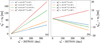Fig. 1 Left panel: de-synchronizations (${\Delta }^{*}={\tau }_{\text{p}}^{*}-{\tau }_s$) and frequency offsets (∆f∗) of four numerically simulated time-aligned orbits with different initial inclinations. Right panel: corrected ${\Delta }_{\text{c}}^{*}={\tau }_{\text{p,c}}^{*}-{\tau }_s$ and $\Delta f_{\text{c}}^{*}$ for the same four simulated orbits by accounting for the deviation of the mean orbital elements in our simulations from the ones required by the time-aligned orbits.

4 Conclusions and discussion

In the context of defining the LRT and the challenges for landing clocks on the surface of the Moon, we show that there exist time-aligned orbits around the Moon with semi-major axes of about 1.5 lunar radii. The readings of an ideal clock in such an orbit can equal the selenoid time, and the same readings could easily be converted to the TCL via a known linear transformation. Therefore, it could be possible to simultaneously realize the LRT options O1 and O2 of Bourgoin et al. (2026) with a single orbital clock. To assess its performance, we conducted a set of numerical simulations. We find that the proper time in the time-aligned orbit under a more realistically lunar gravitational environment would de-synchronize from the selenoid time by up to 190 ns after a year with a frequency offset of 6 × 10⁻¹⁵, which is only 3.75% of the frequency difference in O2 caused by the lunar surface topography. Meanwhile, if we can account for the deviation of the mean orbital elements in our simulations from those required by the time-aligned orbits, we would reduce the de-synchronization and frequency offset by an order of magnitude to 13 ns and 4 × 10⁻¹⁶.

The terrestrial planets may also have their own time-aligned orbits (see Table 3). This would mean that it might be possible to realize the reference times of planets beyond the Earth–Moon system with clocks in these orbits. This shows that options based on the time-aligned orbits are scalable, meaning we could avoid the risks associated with landing clocks on the surfaces of these planets.

Acknowledgements

We acknowledge very useful and helpful comments and suggestions from our anonymous referee. This work is funded by the National Natural Science Foundation of China (Grant Nos. 62394350, 62394351 and 12273116) and the Strategic Priority Research Program on Space Science of the Chinese Academy of Sciences (XDA300103000, XDA30040000, XDA30030000, XDA0350300, XDA30040500 and XDA0350404). J.Z. is funded by the Jiangsu Funding Program for Excellent Postdoctoral Talent (Grant No. 2025ZB724).

References

All Tables

All Figures

Fig. 1 Left panel: de-synchronizations (${\Delta }^{*}={\tau }_{\text{p}}^{*}-{\tau }_s$) and frequency offsets (∆f∗) of four numerically simulated time-aligned orbits with different initial inclinations. Right panel: corrected ${\Delta }_{\text{c}}^{*}={\tau }_{\text{p,c}}^{*}-{\tau }_s$ and $\Delta f_{\text{c}}^{*}$ for the same four simulated orbits by accounting for the deviation of the mean orbital elements in our simulations from the ones required by the time-aligned orbits.

In the text

References

- Ardalan, A. A., & Karimi, R. 2014, Celest. Mech. Dyn. Astron., 118, 75 [Google Scholar]
- Bourgoin, A., Defraigne, P., & Meynadier, F. 2026, Metrologia, 63, 015003 [Google Scholar]
- Formichella, V., Galleani, L., Signorile, G., & Sesia, I. 2021, GPS Solut., 25, 56 [Google Scholar]
- IAU 2024a, Resolution II: “to establish a standard Lunar Celestial Reference System (LCRS) and Lunar Coordinate Time (TCL)”, https://www.iau.org/Iau/Publications/List-of-Resolutions [Google Scholar]
- IAU 2024b, Resolution III: “on the establishment of a coordinated lunar time standard by international agreement”, https://www.iau.org/Iau/Publications/List-of-Resolutions [Google Scholar]
- Kopeikin, S. M., & Kaplan, G. H. 2024, Phys. Rev. D, 110, 084047 [Google Scholar]
- Kouba, J. 2004, GPS Solut., 8, 170 [Google Scholar]
- Nelson, R. A. 2011, Metrologia, 48, S171 [Google Scholar]
- Soffel, M., Klioner, S. A., Petit, G., et al. 2003, AJ, 126, 2687 [Google Scholar]
- Turyshev, S. G., Williams, J. G., Boggs, D. H., & Park, R. S. 2025, ApJ, 985, 140 [Google Scholar]
All Tables
Comparison of nominal mean orbital elements () and mean orbital elements () from our numerical simulations with σ = {a, e, i}.
Mean semi-major axis (āp) of the time-aligned orbits for four terrestrial planets.