| Issue |
A&A
Volume 707, March 2026
|
|
|---|---|---|
| Article Number | L9 | |
| Number of page(s) | 4 | |
| Section | Letters to the Editor | |
| DOI | https://doi.org/10.1051/0004-6361/202659064 | |
| Published online | 06 March 2026 | |
Letter to the Editor
Solar magnetic field stratification from Ca I 4227 Å spectropolarimetric inversions
1
Istituto ricerche solari Aldo e Cele Daccò (IRSOL), Faculty of Informatics, Università della Svizzera italiana 6605 Locarno, Switzerland
2
Euler Institute, Faculty of Informatics, Università della Svizzera italiana 6900 Lugano, Switzerland
3
Institut für Sonnenphysik (KIS) Georges-Köhler-Allee 401a 79110 Freiburg, Germany
4
Faculty of Mathematics, University of Belgrade Studentski Trg 12-16 11000 Belgrade, Serbia
5
Astronomical Observatory Volgina 7 11000 Belgrade, Serbia
★ Corresponding author: This email address is being protected from spambots. You need JavaScript enabled to view it.
Received:
21
January
2026
Accepted:
14
February
2026
Abstract
Spectropolarimetric data for the solar Ca I line at 4227 Å can be acquired from ground-based facilities and theoretical modeling studies have established their sensitivity to magnetic fields across a broad range of atmospheric heights; however, a routinely usable inference tool has been lacking until now. Here, we present the first successful inversion of the spectropolarimetric observations in Ca I 4227 acquired with the ZIMPOL polarimeter at the IRSOL observatory in Locarno. The inversion process incorporates the physical ingredients required for an accurate modeling of these observations, including non-local thermodynamic equilibrium effects, partial frequency redistribution in the general angle-dependent formulation, and the magnetic sensitivity arising from the joint action of the Hanle, Zeeman, and magneto-optical effects. By simultaneously fitting the height-dependent plasma bulk velocity and magnetic field that best reproduce the observed polarization signals, we inferred a physically meaningful stratification of the magnetic field from the photosphere to the low chromosphere. Such inversions demonstrate the feasibility of developing a pipeline to provide information on the magnetism of the low chromosphere and the underlying photosphere from Ca I 4227 spectropolarimetric observations.
Key words: polarization / scattering / Sun: chromosphere / Sun: magnetic fields / Sun: photosphere
© The Authors 2026
 Open Access article, published by EDP Sciences, under the terms of the Creative Commons Attribution License (https://creativecommons.org/licenses/by/4.0), which permits unrestricted use, distribution, and reproduction in any medium, provided the original work is properly cited.
This article is published in open access under the Subscribe to Open model. This email address is being protected from spambots. You need JavaScript enabled to view it. to support open access publication.
1. Introduction
A major challenge in contemporary heliophysics is to accurately measure the magnetic field in the outer layers of the solar atmosphere, a priority goal endorsed by the NASA Heliophysics Science and Technology Roadmap for 2014-2033 and further supported in recent studies (e.g., Carlsson et al. 2019; De Pontieu et al. 2021). The chromosphere poses a particular problem, as traditional magnetic field diagnostics based on the Zeeman effect are less effective in this layer and only a limited number of spectral lines encode information about this region. Recent research has explored alternative approaches, exploiting the magnetic sensitivity of strong resonance lines through the joint action of the Zeeman, Hanle, and magneto-optical (MO) effects (e.g., Trujillo Bueno & del Pino Alemán 2022).
In this context, the polarization of the Ca I resonance line at 4227 Å is noteworthy because its formation is controlled by all the above-mentioned mechanisms, which are sensitive to magnetic fields across a wide range of atmospheric heights. Moreover, spectropolarimetric observations in Ca I 4227 can be performed from the ground; for instance, with ViSP (de Wijn et al. 2022) at the Daniel K. Inouye Solar Telescope (DKIST, Rimmele et al. 2020) or with ZIMPOL (Ramelli et al. 2010) at the IRSOL or GREGOR telescopes (Ramelli et al. 2014). Great efforts have been directed toward observing (e.g., Bianda et al. 2011; Capozzi et al. 2020) and modeling (e.g., Anusha et al. 2011; Supriya et al. 2014; Alsina Ballester et al. 2018; Belluzzi et al. 2024) the polarization of this line, with special focus on the strong signal produced by the scattering of anisotropic radiation (a.k.a. scattering polarization).
In this line, the Zeeman effect produces circular polarization signals when spatially resolved magnetic fields are present in the upper photosphere. The linear scattering polarization signal of this line (the strongest in the visible range of the solar spectrum) shows a sharp peak in the line core and broad lobes in the wings (Gandorfer 2002). The line-core peak is sensitive through the Hanle effect to low chromospheric magnetic fields as low as 5 G (Stenflo 1982; Faurobert-Scholl 1992), while MO effects make the wing lobes sensitive to similarly weak magnetic fields in the lower photosphere (e.g., Alsina Ballester et al. 2018; Capozzi et al. 2022). Building on this research direction, this letter presents pioneering spectropolarimetric inversions of a Ca I 4227 observation with limited spatial and temporal resolutions, targeting a magnetic region situated away from the disk center. We applied the inversion code presented in Janett et al. (2025) and by exploiting the individual signatures of the MO, Zeeman, and Hanle effects, we inferred the vertical stratification of the magnetic field from the photosphere to the low chromosphere.
2. Observation and data reduction
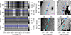 |
Fig. 1. Left: Observed slit-spectra of the Ca I 4227 Stokes vector, whereby the horizontal blue and black dashed lines indicate the spatial regions considered for the inversion. Center and right: Context of the observation given by the continuum and magnetogram (clipped at ±50 gauss) image of HMI on board SDO. The cyan line represents the slit (width not to scale), with the red cross indicating its center, placed at a limb distance of μ = 0.43 (see magenta dashed lines). The blue and black crosses on the slit-spectra images mark the centers of two spatial regions, labeled as A and B, which were considered for the inversion. |
We conducted the observations on October 31, 2024, using the Zurich IMaging POLarimeter (ZIMPOL; Ramelli et al. 2010) in combination with a high-resolution Czerny-Turner slit spectrograph (slit width of 0 5), attached to the 45 cm aperture Gregory Coudé Telescope of the IRSOL observatory in Locarno, Switzerland. We targeted a plage region close to Active Region 13879, with observations commencing at 10:19 UT. During the 10 minutes of observing time, we acquired a total of 320 images, each with a 1 second of exposure time. The slit-center limb distance μ = cos θ = 0.43, with θ as the heliocentric angle, was calibrated by co-aligning our slit-jaw image with a continuum image from the Helioseismic and Magnetic Imager onboard the Solar Dynamics Observatory (HMI/SDO Schou et al. 2012; Pesnell et al. 2012), as shown in Fig. 1. The image spatial sampling is 1
 3 pixel−1, while the spectral sampling is 5.3 mÅ pixel−1, with an estimated spectrally flat stray light contribution of 3%. The seeing was typical for the observatory (1″–3″). To record the four Stokes parameters, ZIMPOL demodulates at 42 kHz on-chip synchronously with a photoelastic modulator combined with an analyzer (see Gandorfer & Povel 1997). The two telescope folding mirrors induce instrumental polarization offsets and circular-to-linear polarization cross-talk, which we minimized by combining ZIMPOL with the slow modulation technique (see details and applications in Zeuner et al. 2022a,b; Esteban Pozuelo et al. 2025), preserving a photon-noise-limited performance.
The acquired images were dark-corrected and polarimetrically calibrated for the fast modulation according to the standard data reduction pipeline. The intensity image was flat-field corrected and residual fringes from the camera micro lenses were reduced1. The resulting Stokes images were combined according to the slow modulation to correct for the polarimetric offsets and circular-to-linear polarization cross-talk (see Zeuner et al. 2022b). A local polarization reference frame was defined for each spatial pixel, with +Q/I parallel to the nearest limb accounting for the limb curvature. The residual Q/I ↔ U/I cross-talk from instrumental uncertainties was corrected by a 3.5° rotation on the Poincaré sphere (6% cross-talk) determined by minimizing the continuum signal in U/I. The photon noise level in the line core is < 0.05% for all Stokes parameters.
Figure 1 presents the fully reduced Ca I 4227 slit spectra. The intensity spectrum exhibits a broad absorption profile with extended wings, accompanied by numerous blends. The Q/I spectrum reveals its distinctive triplet peak structure, characterized by a sharp central peak and prominent lobes in the wings. The Q/I and U/I line-core signals show clear spatial variations along the slit with localized features of both signs, while V/I is much smoother. This indicates that the sensitivity to Hanle and MO effects acting on the linear polarization is stronger than the sensitivity to the Zeeman effect on V/I. Moreover, the substantial U/I signals suggest the presence of resolved chromospheric magnetic fields (e.g., Anusha et al. 2011).
For the inversions, we chose two distinct spatial regions (labeled with A and B in Fig. 1) that exhibit different polarization profiles. Both observations are averaged over a few spatial pixels to enhance the S/N, resulting in a 7 8 spatial resolution.
3. Inversion strategy
The Ca I line at 4227 Å is produced by a resonant transition between the ground level of neutral calcium with a total angular momentum of J = 0 and an upper level with J = 1. The upper level is not radiatively coupled to any level with lower energy apart from the ground level. Due to these atomic properties, the scattering polarization signal of this line can be suitably modeled using a two-level atom with an unpolarized and infinitely sharp lower level (e.g., Alsina Ballester et al. 2018). To accurately model this signal, it is necessary to account for PRD effects in the general angle-dependent formulation (e.g., Janett et al. 2021; Belluzzi et al. 2024). Here, we employed the PRD theory of Bommier (1997a,b), including arbitrary magnetic fields (Hanle-Zeeman regime) and bulk velocities.
As pointed out by Li et al. (2022), outside highly magnetized solar regions (e.g., sunspots), the effect of polarization and magnetic fields on the intensity spectrum is negligible, making it possible to decouple the inversion of the Stokes I profile from the inversion of the polarization profiles. We also note that because of the low spatial and temporal resolution of our observation, the Stokes I profile can be suitably reproduced using a semi-empirical plane-parallel model of the solar atmosphere. Hence, we split our inversion strategy into two distinct steps.
In the first step, we satisfactorily reproduced the observed intensity spectra at μ = 0.43, adopting the atmospheric stratification of temperature and pressure from model C of Fontenla et al. (1993), with micro-turbulent velocities from Fontenla et al. (1991). The synthetic profile was calculated with the RH code (Uitenbroek 2001), considering a multi-level atomic model of calcium and including a series of blends from Fe I, Ti II, Zr I, and Ce II, which influence the extended wings of Ca I 4227.
In the second step, we fitted the height-dependent magnetic field vector and the vertical component of the bulk velocity to the observed fractional polarization profiles, following the approach described in Janett et al. (2025), which is based on the forward engine of the TRAP4 code (Riva et al. 2025). The RH calculation in the previous step also provides the lower-level population of Ca I 4227 and the opacity due to continuum and blends, which are required for the TRAP4 synthesis.
We stress that the adopted strategy is suited due to the low spatio-temporal resolution of the observations. This allows us to consider the thermal stratification of semi-empirical plane-parallel models, instead of recovering it by inverting the intensity spectrum. It also allows us to safely disregard the impact of nonmagnetic axial symmetry-breaking effects, such as horizontal radiative transfer and horizontal bulk velocities (Li et al. 2022). Furthermore, the near-identical intensity spectra of the two observed regions suggest that thermal stratification is similar in both. Consequently, we are confident that the observed spatial variations in the polarization profiles are primarily of magnetic origin. Given the low resolution of the observation, we caution that the inferred vertical bulk velocity should ultimately be interpreted with care. In this context, the vertical bulk velocity likely serves as a nuisance parameter, adjusting the anisotropy and line asymmetry (see also Carlin et al. 2012), rather than representing the actual plasma velocity.
For the forward modeling, we discretized the wavelength interval [4221.4 Å, 4232.0 Å] with 213 spectral points and with a higher density of points in the core of the spectral lines. In the angular dimension, we used seven uniformly distributed points for the azimuth and ten Gauss-Legendre points for the inclination, for a total of 70 angular grid points. We also conducted a solution verification with finer spectral and angular grids, confirming that the numerical errors associated with the employed grids were not relevant. The atmospheric quantities to be inferred were retrieved on a discrete set of spatial nodes and collected in the vector x. These quantities are then reconstructed on the forward problem spatial grid through a f(x) interpolation (e.g., Ruiz Cobo & del Toro Iniesta 1992). For the vertical bulk velocity field, we used two nodes, with a linear interpolation in between. For the magnetic field, we applied the nearest-neighbor interpolation to three nodes located at 300 km (photosphere), 700 km (upper photosphere), and 1100 km (lower chromosphere). According to the Ca I 4227 response functions (e.g, Capozzi et al. 2022), these locations ensure that each node is optimally sensitive to the magnetic field through a different physical mechanism: the deepest node to MO effects, the intermediate one to the Zeeman effect in V/I, and the highest one to the Hanle effect. The magnetic field vector is specified through its longitudinal component B∥ (i.e., along the line of sight), transversal component B⊥ (i.e., in the plane of the sky), and the azimuth of the latter on the plane of the sky ϕB⊥. Bearing in mind that the MO and Zeeman effects are only sensitive to the longitudinal component of the magnetic field, at the two deepest nodes, the transversal component B⊥ is constrained to be zero and ϕB⊥ is consequently undefined. This approach results in a total of 7 free atmospheric parameters, namely, x ∈ ℝ7.
The inversion problem was expressed as the minimization of the sum of squared residuals,
where ri(x) = ωi(Iiout(f(x)) − Iiobs), with i as the index encompassing all the considered Stokes components and all the available wavelengths, and ωi as the weighting coefficient (e.g., del Toro Iniesta & Ruiz Cobo 2016). In the inversion process, we assigned nonzero values to ωi for all wavelengths within ± 0.6 Å of the line center, thus avoiding spectral regions where Ca I 4227 is insensitive to magnetic fields. The nonlinear least-squares problem, argminx S(x), was then addressed iteratively, employing the Matlab Trust Region Reflective algorithm (e.g., Coleman & Li 1996). This minimization method starts with a spatially uniform initial guess (i.e., a horizontal magnetic field of 10 G with zero azimuth and zero bulk velocity) and then reaches a solution that satisfies the predefined convergence criteria. In our approach, the Trust Region Reflective algorithm computes a lightweight Jacobian at each iteration step (see Janett et al. 2025), which allowed us to perform a single inversion in approximately 45 processor minutes (@2.50 GHz). We also apply hard constraints to the inferred atmospheric parameters, requiring B < 125 G and vb < 5 km/s.
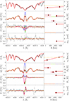 |
Fig. 2. Inversion results for regions A (upper tile) and B (lower tile). Left panels (from top to bottom): Observed (black dots) and inverted (red solid lines) I/Ic, Q/I, U/I, and V/I profiles at μ = 0.43. Right panels (from top to bottom): Two-node fitted vertical bulk velocities and three-node fitted magnetic field components B∥, B⊥, and ϕB⊥. As a reference, we also show the Stokes profiles obtained in the absence of bulk velocity and magnetic fields (orange dashed lines). In addition, we included the synthetic Stokes profiles obtained for the inferred magnetic field stratification after switching off the magnetic field one node at a time (deepest to highest, corresponding to the magenta, green, and blue solid lines, respectively). |
4. Results and conclusions
We simultaneously fitted the height-dependent vertical bulk velocities and magnetic field that best reproduce the polarization signals observed in the two selected regions, with the inversion results shown in Fig. 2. For both cases, we tested the robustness of the inversion by using different initial guesses and consistently obtaining the same solutions. Overall, the inversion aptly reproduces the observed Stokes profiles, successfully capturing all the major non-noise features. The most relevant discrepancy is in the reconstruction of the Q/I minima adjacent to the central line-core peak. To fully appreciate the impact of step 2, Fig. 2 also displays the synthetic Stokes profiles calculated in the absence of vertical bulk velocity and magnetic fields.
The three-node parameterization of the magnetic stratification combined with nearest-neighbor interpolation proved to be crucial for accurately retrieving the observed polarization signals. To clearly disentangle the contributions of the three retrieved magnetic-field layers, Fig. 2 also shows the emergent Stokes profiles obtained by solving the forward problem for the inferred magnetic field stratification while setting to zero the magnetic field at one node at a time. Remarkably, the three nodes isolate the individual signatures of the MO (see near wings of Q/I and U/I), Zeeman (see V/I), and Hanle (see core of Q/I and U/I) effects, respectively.
The inferred longitudinal magnetic field is relatively weak in region A, reaching only a few gauss. In region B, it ranges from a few gauss in the lower photosphere to approximately 15 G in the upper photosphere and lower chromosphere. Notably, the Hanle magnetic sensitivity of the highest node reveals a significant transverse component of the magnetic field of almost 20 G in both regions. This demonstrates that an analysis relying solely on the Zeeman effect can overlook a substantial portion of the magnetic field, specifically its transverse component. We stress that the Hanle sensitivity to relatively weak (and possibly unresolved) magnetic fields yields precious constraints on the magnetic energy content of the solar atmosphere. For context, our inversion-retrieved chromospheric magnetic field of about 20 G corresponds to plasma β ≈ 1 at z = 1100 km in the FAL-C model atmosphere. This inferred magnetic field is consistent with the mean magnetic field strengths obtained from the 3D radiation-magnetohydrodynamic simulations of the quiet Sun internetwork by Przybylski et al. (2025).
While we have ensured a comprehensive modeling of the formation of the Ca I 4227 signals, the reliability of the inferred magnetic fields is affected by several factors, including the observational signal-to-noise ratio, the assumption of a plane-parallel semi-empirical atmospheric model, and the nonuniqueness of the solution (see, e.g., Li et al. 2024, for Hanle effect ambiguities). We also stress that the inferred magnetic field at the two lower nodes yields only the line-of-sight component. Our inversion strategy would greatly benefit from multiline inversions, which would provide a more comprehensive understanding of the stratification of the vector magnetic field.
This letter demonstrates the feasibility of spectropolarimetric inversions of Ca I 4227 to retrieve the magnetic field stratification from the photosphere to the low chromosphere. This diagnostic methodology overcomes the limitations of the Zeeman effect and lays the foundation for a three-dimensional inference of the vector magnetic field, taking advantage of observations with a higher spatial resolution.
Acknowledgments
We thank the anonymous referee for the careful review. GJ and LB acknowledge the financial support by the Swiss National Science Foundation (SNSF) through grants 200021-231308 and CRSK-2_235805. FZ acknowledges funding from the SNSF through grant number PZ00P2_215963. IM acknowledges the financial support from the Serbian Ministry of Science and Technology through the grants 451-03-136/2025-03/200104 and 451-03-136/2025-03/200002. IRSOL is supported by the Swiss Confederation (SEFRI), Canton Ticino, the city of Locarno, and the local municipalities.
References
- Alsina Ballester, E., Belluzzi, L., & Trujillo Bueno, J. 2018, ApJ, 854, 150 [Google Scholar]
- Anusha, L. S., Nagendra, K. N., Bianda, M., et al. 2011, ApJ, 737, 95 [NASA ADS] [CrossRef] [Google Scholar]
- Belluzzi, L., Riva, S., Janett, G., et al. 2024, A&A, 691, A278 [NASA ADS] [CrossRef] [EDP Sciences] [Google Scholar]
- Bianda, M., Ramelli, R., Anusha, L. S., et al. 2011, A&A, 530, L13 [NASA ADS] [CrossRef] [EDP Sciences] [Google Scholar]
- Bommier, V. 1997a, A&A, 328, 706 [NASA ADS] [Google Scholar]
- Bommier, V. 1997b, A&A, 328, 726 [NASA ADS] [Google Scholar]
- Capozzi, E., Ballester, E. A., Belluzzi, L., et al. 2020, A&A, 641, A63 [NASA ADS] [CrossRef] [EDP Sciences] [Google Scholar]
- Capozzi, E., Alsina Ballester, E., Belluzzi, L., & Trujillo Bueno, J. 2022, A&A, 657, A44 [NASA ADS] [CrossRef] [EDP Sciences] [Google Scholar]
- Carlin, E. S., Manso Sainz, R., Asensio Ramos, A., & Trujillo Bueno, J. 2012, ApJ, 751, 5 [NASA ADS] [CrossRef] [Google Scholar]
- Carlsson, M., De Pontieu, B., & Hansteen, V. H. 2019, ARA&A, 57, 189 [Google Scholar]
- Coleman, T. F., & Li, Y. 1996, SIAM J. Optim., 6, 418 [Google Scholar]
- De Pontieu, B., Polito, V., Hansteen, V., et al. 2021, Sol. Phys., 296, 84 [NASA ADS] [CrossRef] [Google Scholar]
- de Wijn, A. G., Casini, R., Carlile, A., et al. 2022, Sol. Phys., 297, 22 [NASA ADS] [CrossRef] [Google Scholar]
- del Toro Iniesta, J. C., & Ruiz Cobo, B. 2016, Liv. Rev. Sol. Phys., 13, 4 [Google Scholar]
- Esteban Pozuelo, S., Asensio Ramos, A., Trujillo Bueno, J., et al. 2025, A&A, 696, A109 [NASA ADS] [CrossRef] [EDP Sciences] [Google Scholar]
- Faurobert-Scholl, M. 1992, A&A, 258, 521 [NASA ADS] [Google Scholar]
- Fontenla, J. M., Avrett, E. H., & Loeser, R. 1991, ApJ, 377, 712 [NASA ADS] [CrossRef] [Google Scholar]
- Fontenla, J. M., Avrett, E. H., & Loeser, R. 1993, ApJ, 406, 319 [Google Scholar]
- Gandorfer, A. 2002, The Second Solar Spectrum: A High Spectral Resolution Polarimetric Survey of Scattering Polarization at the Solar Limb in Graphical Representation. Volume II: 3910 Å to 4630 Å (Zurich: vdf ETH) [Google Scholar]
- Gandorfer, A., & Povel, H. P. 1997, A&A, 328, 381 [NASA ADS] [Google Scholar]
- Janett, G., Ballester, E. A., Guerreiro, N., et al. 2021, A&A, 655, A13 [NASA ADS] [CrossRef] [EDP Sciences] [Google Scholar]
- Janett, G., Milić, I., Riva, F., & Belluzzi, L. 2025, A&A, 701, A80 [NASA ADS] [CrossRef] [EDP Sciences] [Google Scholar]
- Li, H., del Pino Alemán, T., Trujillo Bueno, J., & Casini, R. 2022, ApJ, 933, 145 [NASA ADS] [CrossRef] [Google Scholar]
- Li, H., del Pino Alemán, T., & Trujillo Bueno, J. 2024, ApJ, 975, 110 [Google Scholar]
- Pesnell, W. D., Thompson, B. J., & Chamberlin, P. C. 2012, Sol. Phys., 275, 3 [Google Scholar]
- Przybylski, D., Cameron, R., Solanki, S. K., et al. 2025, A&A, 703, A148 [NASA ADS] [CrossRef] [EDP Sciences] [Google Scholar]
- Ramelli, R., Balemi, S., Bianda, M., et al. 2010, in Ground-based and Airborne Instrumentation for Astronomy III, eds. I. S. McLean, S. K. Ramsay, & H. Takami, SPIE Conf. Ser., 7735, 77351Y [NASA ADS] [Google Scholar]
- Ramelli, R., Gisler, D., Bianda, M., et al. 2014, in Ground-based and Airborne Instrumentation for Astronomy V, eds. S. K. Ramsay, I. S. McLean, & H. Takami, SPIE Conf. Ser., 9147, 91473G [Google Scholar]
- Rimmele, T. R., Warner, M., Keil, S. L., et al. 2020, Sol. Phys., 295, 172 [Google Scholar]
- Riva, F., Janett, G., Belluzzi, L., et al. 2025, A&A, 699, A233 [NASA ADS] [CrossRef] [EDP Sciences] [Google Scholar]
- Ruiz Cobo, B., & del Toro Iniesta, J. C. 1992, ApJ, 398, 375 [Google Scholar]
- Schou, J., Scherrer, P. H., Bush, R. I., et al. 2012, Sol. Phys., 275, 229 [Google Scholar]
- Stenflo, J. O. 1982, Sol. Phys., 80, 209 [Google Scholar]
- Supriya, H. D., Smitha, H. N., Nagendra, K. N., et al. 2014, ApJ, 793, 42 [Google Scholar]
- Trujillo Bueno, J., & del Pino Alemán, T. 2022, ARA&A, 60, 415 [NASA ADS] [CrossRef] [Google Scholar]
- Uitenbroek, H. 2001, ApJ, 557, 389 [Google Scholar]
- Zeuner, F., Belluzzi, L., Guerreiro, N., Ramelli, R., & Bianda, M. 2022a, A&A, 662, A46 [NASA ADS] [CrossRef] [EDP Sciences] [Google Scholar]
- Zeuner, F., Gisler, D., Bianda, M., Ramelli, R., & Berdyugina, S. V. 2022b, in Ground-based and Airborne Instrumentation for Astronomy IX, SPIE Conf. Ser., 12184, 121840T [NASA ADS] [Google Scholar]
The fringes were reduced through a relevance vector machine (github.com/aasensio/rvm) modified by C. J. Díaz Baso (priv. comm.).
All Figures
|
Fig. 1. Left: Observed slit-spectra of the Ca I 4227 Stokes vector, whereby the horizontal blue and black dashed lines indicate the spatial regions considered for the inversion. Center and right: Context of the observation given by the continuum and magnetogram (clipped at ±50 gauss) image of HMI on board SDO. The cyan line represents the slit (width not to scale), with the red cross indicating its center, placed at a limb distance of μ = 0.43 (see magenta dashed lines). The blue and black crosses on the slit-spectra images mark the centers of two spatial regions, labeled as A and B, which were considered for the inversion. |
| In the text | |
|
Fig. 2. Inversion results for regions A (upper tile) and B (lower tile). Left panels (from top to bottom): Observed (black dots) and inverted (red solid lines) I/Ic, Q/I, U/I, and V/I profiles at μ = 0.43. Right panels (from top to bottom): Two-node fitted vertical bulk velocities and three-node fitted magnetic field components B∥, B⊥, and ϕB⊥. As a reference, we also show the Stokes profiles obtained in the absence of bulk velocity and magnetic fields (orange dashed lines). In addition, we included the synthetic Stokes profiles obtained for the inferred magnetic field stratification after switching off the magnetic field one node at a time (deepest to highest, corresponding to the magenta, green, and blue solid lines, respectively). |
| In the text | |
Current usage metrics show cumulative count of Article Views (full-text article views including HTML views, PDF and ePub downloads, according to the available data) and Abstracts Views on Vision4Press platform.
Data correspond to usage on the plateform after 2015. The current usage metrics is available 48-96 hours after online publication and is updated daily on week days.
Initial download of the metrics may take a while.