| Issue |
A&A
Volume 708, April 2026
|
|
|---|---|---|
| Article Number | A70 | |
| Number of page(s) | 14 | |
| Section | Planets, planetary systems, and small bodies | |
| DOI | https://doi.org/10.1051/0004-6361/202554500 | |
| Published online | 30 March 2026 | |
A tension between dust and gas radii: The role of substructures and external photoevaporation in protoplanetary disks
1
University Observatory, Faculty of Physics, Ludwig-Maximilians-Universität München,
Scheinerstr. 1,
81679
Munich,
Germany
2
Dipartimento di Fisica ‘Aldo Pontremoli’, Università degli Studi di Milano,
via G. Celoria 16,
20133
Milano,
Italy
3
Exzellenzcluster ORIGINS,
Boltzmannstr. 2,
85748
Garching,
Germany
4
European Southern Observatory,
Karl-Schwarzschild-Strasse 2,
85748
Garching bei München,
Germany
5
INAF, Osservatorio Astrofisico di Arcetri,
50125
Firenze,
Italy
6
Department of Astronomy and Astrophysics, University of Chicago,
Chicago,
IL
60637,
USA
★ Corresponding author: This email address is being protected from spambots. You need JavaScript enabled to view it.
Received:
12
March
2025
Accepted:
3
February
2026
Abstract
Context. Protoplanetary disk substructures are thought to play a crucial role in disk evolution and planet formation. Population studies of disks large-sample size surveys show that not only substructure, but also their rapid formation, are needed to reproduce the observed spectral indices. Moreover, they enable the simultaneous reproduction of the observed spectral index and size-luminosity distributions.
Aims. This study is aimed at investigating the need for substructures and predicting their characteristics in reproducing the gas-to-dust size ratios observed in the Lupus star-forming region.
Methods. We performed a population synthesis study of gas and dust evolution in disks using a two-population model (two-pop-py) and the DustPy code. We considered the effects of viscous evolution, dust growth, fragmentation, transport, and external photoevaporation. The simulated population distributions were obtained by post-processing the resulting disk profiles of surface density, maximum grain size, and disk temperature.
Results. Although substructures do help in reducing the discrepancy between simulated and observed disk gas-to-dust size ratios, even when accounting for external photoevaporation, they do not fully resolve it. Only specific initial conditions in disks undergoing viscous evolution with external photoevaporation are able to reproduce the observations, highlighting a fine-tuning problem. Even in cases where substructured disks successfully reproduce the dust size and spectral index, they tend to overestimate gas radii.
Conclusions. These results ultimately highlight the main challenge of simultaneously reproducing gas and dust sizes. One possible explanation is that the outermost substructure is linked to the disk truncation radius, which determines the gas radius. Alternatively, it might be the case that substructures are frequent enough to always be located near the outer radius of the gas.
Key words: protoplanetary disks
© The Authors 2026
 Open Access article, published by EDP Sciences, under the terms of the Creative Commons Attribution License (https://creativecommons.org/licenses/by/4.0), which permits unrestricted use, distribution, and reproduction in any medium, provided the original work is properly cited.
This article is published in open access under the Subscribe to Open model. This email address is being protected from spambots. You need JavaScript enabled to view it. to support open access publication.
1 Introduction
The study and strong interest in protoplanetary disk substructures have been fueled by the advent of the Atacama Large Millimeter/Sub-Millimeter Array (ALMA) and its high-resolution observations. The iconic image of HL Tau, captured by ALMA Partnership (2015), not only provided the first direct image of a protoplanetary disk, but also revealed, for the first time, the presence of substructures. In particular, surveys such as the Disk Substructures at High Angular Resolution Project (DSHARP; Andrews et al. 2018a; Huang et al. 2018), Long et al. (2018), and the Ophiuchus DIsc Survey Employing ALMA (ODISEA; Cieza et al. 2019, 2021) have shown that optically thick substructures are ubiquitous in bright and extended disks. This finding has sparked further interest in investigating the physical processes that give rise to such substructures and their implications for disk evolution and planet formation. Among the various mechanisms proposed to explain the origin of substructures in protoplanetary disks (see, e.g., Bae et al. 2023), the most widely recognized scenario assumes that substructures observed in Class II disks are created by the presence of planets or protoplanets within the disk. This hypothesis is supported by kinematic evidence (Teague et al. 2018; Pinte et al. 2018; Izquierdo et al. 2022) and by detection of planets within gaps, such as in PDS70 (Müller et al. 2018; Keppler et al. 2018). The interest in protoplanetary disk substructures extends beyond the observational findings. Indeed, it also arises from theoretical considerations, as they may help address several open key problems in disk evolution and planet formation theories. In particular, the fact that dust radially drifts inward in a disk as a result of the different velocities between the dust and gas in the disk (Weidenschilling 1977) is a well-known open question of the field. Solid particles migrate too quickly in smooth disks due to the high efficiency of the radial drift (Takeuchi & Lin 2002, 2005), challenging the formation of planetesimals and leading to mismatches in spectral index predictions (Birnstiel et al. 2010b; Pinilla et al. 2013) and size-luminosity distributions (Tripathi et al. 2017; Andrews et al. 2018b; Rosotti et al. 2019a) compared to observations. Substructures, particularly the presence of local maxima in the pressure profile of the disk, can mitigate solid particle migration or completely trap them at the pressure maximum (Pinilla et al. 2012, 2013). If the substructure trapping mechanism is effective, solid particles accumulate at the pressure maximum enhancing the local dust-to-gas ratio (Drążkowska et al. 2016; Yang et al. 2017), thus creating a favorable region for planetesimal formation (Youdin & Shu 2002; Youdin & Lithwick 2007). Additionally, substructures provide an ideal environment for planet formation by promoting processes like streaming instability and pebble accretion (Morbidelli 2020; Guilera et al. 2020; Chambers 2021; Lau et al. 2022; Jiang & Ormel 2023). They also offer solutions to the migration problem (e.g., Matsumura et al. 2017; Liu et al. 2019; Bitsch et al. 2019; Lau et al. 2024b), such as explaining the location of Jupiter within the Solar System (Lau et al. 2024a).
The quick disappearance of large-sized dust particles in disks is not the only challenging problem of disk evolution. The gas component is also evolving with time, and the gas size, commonly measured as the radius enclosing 68%, 90%, or 95% of the molecular emission of CO, is also studied as a way to probe disk evolution (Ansdell et al. 2018; Trapman et al. 2020, 2022). Different mechanisms of disk evolution predict different pathways for gas disk sizes. In a scenario where accretion is driven by viscosity, disk sizes should globally increase with time (the so-called viscous spreading effect) to conserve angular momentum, while such expansion is not required in case of magnetohydro-dynamic (MHD) disk winds removing angular momentum from the disk (for a review, see, e.g., Manara et al. 2023). This is not the end of the story, as environmental effects, such as multiplicity (e.g., Zagaria et al. 2023) as well as external and internal photoevaporation (e.g., Clarke 2007; Winter & Haworth 2022; Anania et al. 2025b), can reduce or modify the size of a disk, with substantial consequences for the evolution of disks.
Trying to reproduce the dust and gas sizes simultaneously provides a direct test of both the efficiency of radial drift and the mechanisms driving disk evolution. This comparison is based on values measured observationally in several star-forming regions (Sanchis et al. 2021 for Lupus, Long et al. 2022 for Taurus). For the measured sources, the vast majority of the disks in the sample show a ratio of RCO/Rdust between 2–4, with a few outliers (i.e., about 15%) displaying RCO/Rdust > 4. This hints at a similar evolution mechanism for the two star-forming regions. However, theoretical analysis (Toci et al. 2021) modeling studies of the evolution of protoplanetary disks assuming viscous evolution, grain growth, and pure radial drift have reported that for a broad range of disks values, the value of RCO/Rdust becomes >5 after a short time. Substructures have also been proposed as a possible solution to this discrepancy between the observed and simulated gas-to-dust size ratios in protoplanetary disks. Toci et al. (2021) invoked the presence of unresolved or undetected substructures in most (or all) protoplanetary disks as the most likely explanation for reconciling the simulated gas-to-dust size ratios with the observed values. Indeed, the discrepancy between the small observed size ratios (i.e., RCO/Rdust < 5) and the high simulated size ratios (i.e., RCO/Rdust > 5) could potentially be addressed by increasing the disk dust size, Rdust, through the presence of substructures within the disk. Based on their population synthesis study, Delussu et al. (2024) showed that substructures, along with their rapid formation processes, are needed to produce small values of the spectral index in the range of the observed ones, and they allow the observed distributions for both spectral index and size-luminosity to be reproduced.
In this work, we aim to extend the population synthesis study of Delussu et al. (2024) by investigating whether, as proposed by Toci et al. (2021), substructures can provide a solution to the gas-to-dust size ratio problem. Moreover, we aim to understand whether it is possible to match the gas-dust size, size-luminosity, and spectral index distributions at the same time and what initial disk parameters are required for that. Furthermore, we consider the impact of the stellar formation environment, exploring whether the external photoevaporation of the disk caused by the ultraviolet (UV) radiation emitted by OBA-type stars could explain the RCO/Rdust observed in the population of disks in the Lupus region. The UV radiation induces outside-in photoevaporation of the outermost disk regions, which are poorly gravitationally bound to the central star (e.g., Adams et al. 2004, Winter & Haworth 2022). The far-ultraviolet (FUV) component dominates over the extreme UV in the nearby regions ~200 pc from the Sun, which host few massive stars (mainly of late-type B and early-type A). However, indirect evidence and models show that even a moderate FUV field (1–10 G0) can significantly affect disk evolution (e.g., van Terwisga & Hacar 2023), with photo-evaporative mass loss rates that depend on the stellar mass and disk parameters (e.g., Haworth et al. 2023).
This paper is structured as follows. In Sect. 2 we describe our computational models for the evolution of the disk and introduce the analysis method exploited to compare to disk observations. Section 3 introduces the main results obtained and the comparison to the observed distributions. We first introduce the population synthesis results obtained with the two-pop-py model and then the results obtained for a small set of test disks using the code DustPy and in the presence of external photoevaporation. In Sect. 4 we discuss our results and their implications. Section 5 presents our conclusions.
2 Methods
The two-population model (two-pop-py) by Birnstiel et al. (2012) and Birnstiel et al. (2015) and DustPy code (Stammler & Birnstiel 2022) were employed to perform numerical simulations to describe the gas and dust evolution in a protoplanetary disk. In the following, we describe the main characteristics of the two-pop-py1 model and DustPy2 code, along with a description of how external photoevaporation is implemented in DustPy. The observables examined in this work will also be introduced, along with the process applied to evaluate each of them for every simulated disk.
2.1 Two-pop-py model
Two-pop-py is a tool that is well suited for disk population studies since it captures the dust surface density evolution, the viscous evolution of the gas, and the particle size with good accuracy. Since it is based on a set of simple equations, it allows us to perform a single simulation quickly (on the order of seconds), making it computationally efficient and allowing for the execution of large numbers of simulations within a reasonable amount of time. The two-pop-py model, as implemented and described in Delussu et al. (2024), was used in this work. For an in-depth discussion, we refer to Delussu et al. (2024). A summary of its key elements is given below:
The protoplanetary gas disk is evolved according to the viscous disk evolution equation (Lüst 1952; Lynden-Bell & Pringle 1974) using the turbulent effective viscosity as parameterized in Shakura & Sunyaev (1973).
Adopting the two-population model described in Birnstiel et al. (2012), we can evolve the dust surface density assuming that the small dust is tightly coupled to the gas, while the large dust particles can decouple from it and drift inward.
-
The initial gas surface density follows the Lynden-Bell & Pringle (1974) self-similar solution,
![Mathematical equation: $\[\Sigma_g(r)=\Sigma_0\left(\frac{r}{r_{\mathrm{c}}}\right)^{-p} \exp \left[-\left(\frac{r}{r_{\mathrm{c}}}\right)^{2-p}\right],\]$](/articles/aa/full_html/2026/04/aa54500-25/aa54500-25-eq1.png) (1)
(1)where the normalization parameter
![Mathematical equation: $\[\Sigma_{0}=(2-p) M_{disk} / 2 \pi r_{\mathrm{c}}^{2}\]$](/articles/aa/full_html/2026/04/aa54500-25/aa54500-25-eq2.png) is set by the initial disk mass, Mdisk, rc denotes the so-called characteristic radius of the disk, and p is the initial surface density power law exponent, with p set to 1 for the initial profiles of all the disks.
is set by the initial disk mass, Mdisk, rc denotes the so-called characteristic radius of the disk, and p is the initial surface density power law exponent, with p set to 1 for the initial profiles of all the disks. We adopted a passive irradiated disk temperature model (Kenyon et al. 1996) with a disk floor temperature set to 10 K. No viscous heating or other processes have been considered.
Both disks without (referred to as smooth disks) and with substructure were examined. The substructure was modeled as a gap due to the presence of a planet inserted in the disk. To mimic the presence of a planetary gap, we subdivided the α-viscosity parameter into two different values: αgas and αdust. The presence of the planet was modeled as a local variation of the αgas parameter. Given the inverse proportionality between αgas and Σg in a steady-state regime, a bump in the αgas profile results in a gap in the Σg profile, effectively simulating the presence of a planetary gap. Moreover, this approach preserves the viscous evolution of Σg. We adopted the Kanagawa et al. (2016) prescription to model the planetary gaps created in the disk.
In this work, the 1D disk was spatially modeled with a logarithmic radial grid that ranges from 0.05 au to 10 000 au. The main parameters of the grid model are presented in Table 1. A total of 105 simulations were performed for each population synthesis. To map the entire parameter space, the set of initial conditions adopted for each disk was constructed randomly drawing each parameter from a probability distribution function (PDF). As in Delussu et al. (2024), the main parameters taken into account to describe both smooth and substructured disks are: disk mass (Mdisk), stellar mass (Mstar), disk characteristic radius (rc), viscosity parameter (α), and fragmentation velocity (vfrag). The stellar mass values were drawn from a functional form of the initial mass function (IMF) proposed by Maschberger (2013). Substructured disks are characterized by three additional parameters: the mass of the planet creating the gap (mp), the time (tp) at which the planet was inserted, and the position (rp) of the planet within the disk. Table 2 shows the range adopted for each parameter and the corresponding PDFs.
2.2 DustPy and external photoevaporation
Given that external photoevaporation is not yet available in two-pop-py, to perform numerical simulations of disks undergoing external photoevaporation, we used the existing and tested implementation of DustPy (Stammler & Birnstiel 2022) integrated with an external module that includes the effect of an external FUV field (Gárate et al. 2024; Anania et al. 2025a). DustPy simulates the radial evolution of gas and dust in a viscous disk, considering a distribution of particle species subject to advection, diffusion, grain growth by coagulation, and fragmentation based on Birnstiel et al. (2010a). Here, Σg, evolves accordingly with the Lin & Papaloizou (1986) and Trilling et al. (1998) advection-diffusion equation under the influence of axis-symmetrical torque deposition, where we included an extra term to account for the loss of material in external winds,
![Mathematical equation: $\[\frac{\partial \Sigma_{\mathrm{g}}}{\partial t}=\frac{3}{r} \frac{\partial}{\partial r}\left[r^{1 / 2} \frac{\partial}{\partial r}\left(v \Sigma_{\mathrm{g}} r^{1 / 2}\right)-\frac{2 \Lambda \Sigma_{\mathrm{g}}}{3 \Omega_{\mathrm{K}}}\right]-\dot{\Sigma}_{\mathrm{ext}},\]$](/articles/aa/full_html/2026/04/aa54500-25/aa54500-25-eq3.png) (2)
(2)
where ![Mathematical equation: $\[\nu=\alpha c_{\mathrm{s}}^{2} / \Omega_{\mathrm{K}}\]$](/articles/aa/full_html/2026/04/aa54500-25/aa54500-25-eq4.png) is the viscosity, Λ is the specific angular momentum injection rate, and
is the viscosity, Λ is the specific angular momentum injection rate, and ![Mathematical equation: $\[\dot{\Sigma}_{\text {ext}}\]$](/articles/aa/full_html/2026/04/aa54500-25/aa54500-25-eq5.png) accounts for the rate of mass lost in external photo-evaporative winds. The photo-evaporative mass loss rate was evaluated performing a bi-linear interpolation of the FRIEDv2 grid (Haworth et al. 2023), where we assumed interstellar-medium-like polycyclic aromatic hydrocarbons for interstellar-medium-like dust. Specifically, following the numerical implementation of Sellek et al. (2020), the grid was interpolated by fixing the stellar mass and the FUV flux at the outer disk edge, using the disk surface density at each radial position. At each time step, the disk radial position corresponding to the maximum mass loss rate generally defines a truncation radius (which corresponds to the optically thin or thick wind transition in the disk). To simulate the outside-in disk depletion caused by external photoevaporation, the disk material outside the truncation radius is removed accordingly to Sellek et al. (2020). The model takes into account the fact that external photoevaporation influences the dust component, where dust grains smaller than a certain size limit (depending on the stellar and disk parameters) are entrained in winds (Facchini et al. 2016). The study performed by Gárate et al. (2024) showed that dust substructures forming in disks have the capacity to survive the outside-in disk depletion only if they are placed inside the truncation radius of external photoevaporation.
accounts for the rate of mass lost in external photo-evaporative winds. The photo-evaporative mass loss rate was evaluated performing a bi-linear interpolation of the FRIEDv2 grid (Haworth et al. 2023), where we assumed interstellar-medium-like polycyclic aromatic hydrocarbons for interstellar-medium-like dust. Specifically, following the numerical implementation of Sellek et al. (2020), the grid was interpolated by fixing the stellar mass and the FUV flux at the outer disk edge, using the disk surface density at each radial position. At each time step, the disk radial position corresponding to the maximum mass loss rate generally defines a truncation radius (which corresponds to the optically thin or thick wind transition in the disk). To simulate the outside-in disk depletion caused by external photoevaporation, the disk material outside the truncation radius is removed accordingly to Sellek et al. (2020). The model takes into account the fact that external photoevaporation influences the dust component, where dust grains smaller than a certain size limit (depending on the stellar and disk parameters) are entrained in winds (Facchini et al. 2016). The study performed by Gárate et al. (2024) showed that dust substructures forming in disks have the capacity to survive the outside-in disk depletion only if they are placed inside the truncation radius of external photoevaporation.
Due to the higher computational costs of DustPy compared to two-pop-py, we switched from a population synthesis study to a test population study of disks based on the constraints on the parameter space placed by two-pop-py simulations (Delussu et al. 2024) of non-photoevaporating disks for the initial conditions needed to reproduce the observed distributions of spectral index and size-luminosity. The extent of the radial grid, the dust particle distribution and the fragmentation velocity are set as in two-pop-py simulations. In total, we explored the parameter space by performing 27 simulations, considering all possible combinations of the parameter values listed in Table 3. In the simulations including external photoevaporation, we assumed that the disks are subject to a constant external FUV flux of 4 G0, which is the average FUV flux experienced by disk-hosting stars in the Lupus star-forming region (Anania et al. 2025b). The simulated disks are let evolve up to the age of 3 Myr to compare with the Lupus disk population.
As for the study conducted with two-pop-py (Sect. 2.1), the substructures in DustPy were also modeled as a gap arising from the presence of a planet inserted in the disk. We imposed the planetary gap through the radial gas flux induced by a torque profile, rather than modifying the viscosity α-parameter. This approach allows us to avoid the issue of unrealistically high gas velocities with a deep planetary gap, which could arise from low gas surface density caused by disk dissipation due to external photoevaporation. Appendix A shows a comparison between DustPy and two-pop-py for substructured test disks. While minor differences are observed near the planet-induced substructure and modestly affect the spectral indices, the dust and gas disk radii, the main observables considered in this study, are in good agreement, and the main conclusions are therefore preserved. Given its more detailed treatment of substructure formation, we chose to adopt DustPy for the remainder of the study, as detailed below. The angular momentum injection rate Λ in Eq. (2) can be derived by assuming a steady state with the target surface density profile and an unchanged steady-state accretion rate. When neglecting the photoevaporation term, Eq. (2) can be expressed as
![Mathematical equation: $\[\frac{\partial \Sigma_{\mathrm{g}}}{\partial t}=\frac{3}{r} \frac{\partial}{\partial r}\left[r \Sigma_{\mathrm{g}}(v_v+v_{\Lambda})\right],\]$](/articles/aa/full_html/2026/04/aa54500-25/aa54500-25-eq6.png) (3)
(3)
with the accretion velocity as
![Mathematical equation: $\[v_\nu=-\frac{3 \nu}{r} \frac{\partial ~\log }{\partial ~\log~ r}\left(\Sigma_{\mathrm{g}} r^{1 / 2} \nu\right),\]$](/articles/aa/full_html/2026/04/aa54500-25/aa54500-25-eq7.png) (4)
(4)
and the additional velocity due to the torque injection,
![Mathematical equation: $\[v_{\Lambda}=\frac{2 \Lambda}{\Omega_{\mathrm{K}} r}.\]$](/articles/aa/full_html/2026/04/aa54500-25/aa54500-25-eq8.png) (5)
(5)
The condition for the planetary gap to avoid impeding disk accretion can be expressed as
![Mathematical equation: $\[\Sigma_{\mathrm{g}, \mathrm{eq}}(v_{v, \mathrm{eq}}+v_{\Lambda})=\Sigma_{\mathrm{g}, 0} v_{\nu, 0},\]$](/articles/aa/full_html/2026/04/aa54500-25/aa54500-25-eq9.png) (6)
(6)
where Σg,0 represents the unperturbed gas surface density, vν,0 is the unperturbed accretion velocity, while Σg,eq and vν,eq denote the gas surface density and accretion velocity at the steady state with the imposed gap. Starting from Eq. (4), defining the target surface density profile as
![Mathematical equation: $\[f(r) \equiv \frac{\Sigma_{\mathrm{g}, \mathrm{eq}}}{\Sigma_{\mathrm{g}, 0}},\]$](/articles/aa/full_html/2026/04/aa54500-25/aa54500-25-eq10.png) (7)
(7)
and given that ∂(Σg,0 ν)/∂r = 0 under the assumption of a constant disk accretion rate, vν,eq is given by
![Mathematical equation: $\[v_{\nu, \mathrm{eq}}=-\frac{3 v}{r} \frac{\partial ~\log }{\partial ~\log~ r}\left(f \Sigma_{\mathrm{g}, 0} r^{1 / 2} \nu\right)\]$](/articles/aa/full_html/2026/04/aa54500-25/aa54500-25-eq11.png) (8)
(8)
![Mathematical equation: $\[=-\frac{3 \nu}{r}\left(\frac{\partial ~\log~ f}{\partial ~\log~ r}+\frac{1}{2}\right),\]$](/articles/aa/full_html/2026/04/aa54500-25/aa54500-25-eq12.png) (9)
(9)
and vν,0 is
![Mathematical equation: $\[v_{\nu, 0}=-\frac{3 \nu}{2 r}.\]$](/articles/aa/full_html/2026/04/aa54500-25/aa54500-25-eq13.png) (10)
(10)
Exploiting Eq. (6), it follows that
![Mathematical equation: $\[v_{\Lambda}=\frac{v_{\nu, 0}}{f(r)}-v_{\nu, \mathrm{eq}}\]$](/articles/aa/full_html/2026/04/aa54500-25/aa54500-25-eq14.png) (11)
(11)
![Mathematical equation: $\[=-\frac{3 \nu}{r}\left(\frac{1}{2 f}-\frac{\partial ~\log~ f}{\partial ~\log~ r}-\frac{1}{2}\right).\]$](/articles/aa/full_html/2026/04/aa54500-25/aa54500-25-eq15.png) (12)
(12)
To implement this in DustPy, an external source is applied and calculated with vΛ, following the procedure described in Lau et al. (2025). For the profile f, we adopted the planetary gap profile by Kanagawa et al. (2016), as for the two-pop-py model (Sect. 2.1).
Fixed parameters adopted for two-pop-py model.
Disk initial parameters adopted for two-pop-py population synthesis.
Disk initial parameters adopted for the DustPy simulations.
2.3 Observables
By postprocessing the resulting profiles (surface density, maximum grain size, and disk temperature) of the simulated disks, we obtained the simulated population distribution for the disk dust radii, disk gas radii, millimeter fluxes, and spectral indices. In the following we describe the process applied to evaluate each of these observables for every simulated disk.
2.3.1 Millimeter fluxes
The disk fluxes were evaluated following the procedure described in Delussu et al. (2024), that is, adopting the Miyake & Nakagawa (1993) scattering solution of the radiative transfer equation and the modified Eddington–Barbier approximation (Birnstiel et al. 2018). Delussu et al. (2024) studied the effects of different opacities (Ricci compact Rosotti et al. 2019a, DSHARP Birnstiel et al. 2018, DIANA Woitke et al. 2016), and showed that only the Ricci compact opacity results in a match of the observed spectral index distribution. Thus, we adopted the Ricci compact opacity model for our analysis.
2.3.2 Dust radii
One of the challenges in characterizing protoplanetary disks is defining their size (see Miotello et al. 2023, for a recent review). As discussed in Tripathi et al. (2017) and Rosotti et al. (2019b), the characteristic radius, rc, is not an optimal choice as a size indicator for disks. In large sample surveys, the millimeter surface brightness profile of observed disks is measured; thus, we followed the procedure of defining an empirical radius, commonly referred to as the effective disk radius, Reff, which represents the radius encompassing a specified fraction of the total flux emitted by the disk. The two most commonly adopted choices are R68% and R90%, with the the radii enclosing 68% and 90% of the total disk flux, respectively. As shown in Sanchis et al. (2020), R68% is a safer choice, as it is usually characterized by a smaller dispersion. Based on the radii provided in the observed samples; R68% was evaluated for the comparison to the observed size-luminosity distribution (Andrews et al. 2018b), while R90% was evaluated for the comparison to the observed gas and dust radii distribution (Sanchis et al. 2021).
2.3.3 Gas radii
Estimating the disk gas radii is even more challenging than estimating dust radii, as molecular emission lines are faint in the outer regions of protoplanetary disks. Additionally, deep gas observations are rarer as they are more time-consuming than dust continuum observations. Given their brighter and more optically thick emission, CO rotational emission lines (particularly the 12CO lines) are the most commonly used tracers for disk gas radii estimates. Given that we sought to compare our simulated disks to the observed size distribution of disks of the Lupus star-forming region presented in Sanchis et al. (2021), which provides the radius enclosing the 90% of the total flux emission of the 12CO tracer, we assumed 12CO as disk gas size tracer and RCO,90% as the gas radius for each of the simulated disks. As shown in Toci et al. (2023), RCO,90% is well-approximated by the radial location where the disk surface density equals a certain critical value, inhibiting 12CO self-shielding.
We can evaluate the disk gas radius RCO,90% starting from the gas critical column density threshold formula obtained by Trapman et al. (2023):
![Mathematical equation: $\[\mathrm{N}_{\text {gas,crit}}=10^{21.27-0.53 log _{10} \mathrm{L}_{\star}}\left(\frac{\mathrm{M}_{\text {gas}}}{\mathrm{M}_{\odot}}\right)^{0.3-0.08 log _{10} \mathrm{L}_{\star}} \mathrm{cm}^{-2}.\]$](/articles/aa/full_html/2026/04/aa54500-25/aa54500-25-eq16.png) (13)
(13)
Given the gas critical column density threshold, the critical surface density of the 12CO tracer is given by
![Mathematical equation: $\[\Sigma_{\text {crit }}=10 \mu_{\text {gas}} N_{\text {gas,crit}},\]$](/articles/aa/full_html/2026/04/aa54500-25/aa54500-25-eq17.png) (14)
(14)
where μgas is the mean molecular weight of the gas in the disk; we adopted the standard value for protoplanetary disks (i.e., μgas ~ 2.3μH = 1.15μH2). As in Eq. (13), the initial carbon abundance is assumed to be 10−4; we accounted for extra carbon depletion due to CO freeze-out and photodissociation by multiplying the critical surface density by a factor of 10. The gas radius RCO,90% was then evaluated as the outermost radius for which the gas surface density profile obtained for each simulated disk equals its critical surface density.
2.3.4 Spectral index
The spectral index is defined as the slope of the (sub)millimeter spectral energy distribution of the dust emission
![Mathematical equation: $\[\alpha_{m m}=\frac{d log F_\nu}{d log \nu},\]$](/articles/aa/full_html/2026/04/aa54500-25/aa54500-25-eq18.png) (15)
(15)
where Fν is the disk-integrated flux at a given frequency, ν3; thus, αmm is the disk-integrated spectral index. Since we are typically working with frequencies that are very close to each other, Eq. (15) can be written as
![Mathematical equation: $\[\alpha_{m m}=\frac{log(F_{\nu, 2} / F_{\nu, 1})}{log(\nu_2 / \nu_1)}.\]$](/articles/aa/full_html/2026/04/aa54500-25/aa54500-25-eq19.png) (16)
(16)
Equation (16) was applied to determine the spectral index for every simulated disk. Since we are comparing our simulated spectral index distribution to the observed Lupus region sample adopted in Tazzari et al. (2021b), which is a collection of disks detected at 0.89mm (Ansdell et al. 2016) and 3.1 mm (Tazzari et al. 2021b), we considered λ2 = 0.89 mm and λ1 = 3.10 mm.
3 Results
The following section contains the main results obtained through our analysis. Section 3.1 presents the results obtained for the population synthesis produced with two-pop-py for the reproducibility of the gas and dust size observed distribution. In Sect. 3.2 we show the results obtained for a test population of disks exploiting DustPy code with the implementation of external photoevaporation. To compare the simulated distributions with the observed ones, a potential age spread of the simulated disks was considered. Specifically, for each simulated disk, the observables used to construct the overall simulated distributions were randomly selected from the snapshots at 1 Myr, 2 Myr, and 3 Myr. Our simulated gas and dust size distribution is compared to the observed sample reported in Long et al. (2022) for the Lupus region, while the simulated spectral index distributions are compared to the observed sample from Tazzari et al. (2021b). The latter includes disks detected at 0.89 mm (Ansdell et al. 2016) and 3.1 mm (Tazzari et al. 2021b). The simulated size-luminosity distribution is compared to the observed sample of the Lupus region reported in Andrews et al. (2018b).
3.1 Population synthesis results with two-pop-py
The main focus of this study, conducted using two-pop-py model, is to investigate the population synthesis results for the gas and dust size distribution of smooth and substructured disks and to assess the validity of the solution proposed by Toci et al. (2021); namely, that substructures can solve the discrepancy between models and observations. Figure 1 shows the clear difference found between smooth and substructured disks. If we consider the entire parameter space of the initial conditions adopted and reported in Table 2, we can observe the first important indications obtained through our simulations, as detailed below:
Smooth disks produce a large Rgas(90%)/Rdust(90%) compared to observations. This result confirms and extends to the broader level of a disk population synthesis the result previously obtained by Toci et al. (2021).
Substructured disks, either with one or two substructures, produce a size distribution shifted towards lower Rgas(90%)/Rdust(90%). For both one and two substructures, the bulk of the population lies around Rgas(90%)/Rdust(90%) ~ 4.
The presence of substructure(s) in the disks helps narrow the gap between theoretical models and observations, but it does not fully resolve the discrepancy.
For completeness, Figure 1 also presents the spectral index and size-luminosity distributions associated with the three types of disks examined. As already shown in Delussu et al. (2024), only substructured disks are capable of producing spectral indices that populate the observed spectral index region. Therefore, Figure 1 illustrates how smooth disks fail to reproduce two of the three observed distributions examined. However, it also highlights a tension for substructured disks between the favorable results for the spectral index and size-luminosity distributions, which can be simultaneously reproduced by restricting the parameter space of the initial conditions of the simulated disks (Delussu et al. 2024), and the discrepancy between simulated and observed size distribution.
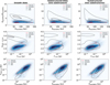 |
Fig. 1 Gas-dust size distribution (first row), spectral index distribution (second row), and size-luminosity distribution (third row) for the parameter space of the initial conditions selecting disks with a spectral index of 0 ≤ α0.89–3.1 mm ≤ 4, 10−3 Jy ≤ F1mm ≤ 10 Jy, 10−3 Jy ≤ F0.89mm ≤ 10 Jy, 100.1 au ≤ Rdust(68%) ≤ 102.6 au, 1 au ≤ Rdust(90%) ≤ 200 au, and 0.1 ≤ Rgas(90%)/Rdust(90%) ≤ 20. Left plots: Smooth disks. Middle plots: Substructured disks with one planet randomly inserted in a range between 0.1–0.4 Myr from the start of the disk evolution. Right plots: substructured disks with two planets randomly inserted in a range between 0.1–0.4 Myr (innermost planet) and between 0.5–0.8 Myr (outermost planet) from the start of the disk evolution. Heatmap of the observed disks with the black dots representing each single observed disk. The black and red lines refer to the simulated results and the observational results, respectively. In particular, the continuous lines encompass 30% of the cumulative sum of the disks produced from the simulations or observed. The dashed lines encompass the 90% instead. |
3.2 DustPy and external photoevaporation results
Having determined that the mere presence of substructures in protoplanetary disks is insufficient to solve the size distribution problem, we carried out a further study to investigate whether external photoevaporation (in conjunction with substructures) might be the necessary ingredient to reconcile observations and simulations. Nevertheless, given that external photoevaporation is not yet available in two-pop-py, we switched from a population synthesis study to a test population study of disks conducted with DustPy, where the effect of external photoevaporation was included in addition to viscous evolution. We assumed that the disks are exposed to a constant external FUV flux of 4 G0, which corresponds to the average FUV flux experienced by disk-hosting stars in the Lupus star-forming region (Anania et al. 2025b). Figure 2 shows the behavior of some substructured test disks in the Rgas(90%)/Rdust(90%) versus Rdust(90%) space in the regime of low viscosity (i.e., α = 10−3.5):
Disks hosted by a solar mass star evolve towards high ratios of Rgas(90%)/Rdust(90%), as shown in the right panels of Fig. 2. The disk decreases in Rdust(90%) rapidly settling to a fixed value corresponding to the location of the substructure; nevertheless, Rgas(90%)/Rdust(90%) increases over time because these disks experience viscous spreading or just slightly reduces their Rgas(90%) due to a small effect of the external photoevaporation.
Disks hosted by a star with Mstar = 0.3 M⊙ and with a small characteristic radius of rc = 20 au evolve towards high ratios of Rgas(90%)/Rdust(90%). This is because they experience viscous spreading because their external photoevaporation truncation radius is placed too farther away (~100 au) to impact the disk evolution. This is shown in the left panels of Fig. 2.
The left panels of Fig. 2 show that medium (rc = 50 au) and large (rc = 100 au) disks hosted by a star with Mstar = 0.3 M⊙ evolve towards small ratios of Rgas(90%)/Rdust(90%), falling close to or inside the observed region.
Having established that small-size disks (i.e., rc = 20 au) and disks hosted by a solar-mass star do not exhibit the desired behavior, we focused on medium (i.e., rc = 50 au) and large (i.e., rc = 100 au) disk size cases hosted by a star of mass Mstar = 0.3 M⊙. In Fig. 3, we can see the impact of the external photoevaporation on the behavior of these disks. Disks completely revert their behavior in the absence of external photoevaporation moving towards high Rgas(90%)/Rdust(90%) ratios as they experience viscous spreading in Rgas(90%) in the absence of external photoevaporation. The first decrease in Rgas(90%)/Rdust(90%) experienced by the disk with mass Mdisk = 0.01 Mstar and rc = 100 au is simply because Rdust(90%) settles towards the location of the substructure; in this case, it happens to produce an increase in Rdust(90%). However, also this disk is affected by spreading in Rgas(90%), which (combined with the stable Rdust(90%) produced by the presence of the substructure) leads to an increase of Rgas(90%)/Rdust(90%) over time. In Figs. 4 and 5, we give an extension and in-depth investigation of our discussion focused on the disk cases that have proven successful thus far in their behavior in the Rgas(90%)/Rdust(90%) versus Rdust(90%) space.
Medium disks (i.e., rc = 50 au) experience a continuous reduction of their Rgas(90%)/Rdust(90%) for all the substructures locations examined, as shown in Fig. 4. However, if we extend our investigation to the behavior of these disks in the spectral index and size-luminosity space we immediately notice the emergence of some problems. All “lighter” disks (i.e., with an Mdisk = 0.01 Mstar) produce large values of spectral indexes and extremely low fluxes. The same problem is displayed by the more massive disks (i.e., with an Mdisk = 0.1 Mstar) if the substructure is placed at or beyond the characteristic radius. Nevertheless, placing the substructure too far inside does not yield beneficial results, as demonstrated by the case of rp = 0.5 rc. This configuration produces a smaller Rdust(90%), which fails to sufficiently decrease the Rgas(90%)/Rdust(90%) ratio.
Figure 4 shows that if the substructure is placed at an intermediate position (i.e., rp = 0.7 rc) and Mdisk = 0.1 Mstar, the disk behaves well in all the parameter space taken into account. Nevertheless, it introduces a warning that we face a fine-tuning problem.
Figure 5 shows that large disks (i.e., rc = 100 au) experience a continuous reduction of their Rgas(90%)/Rdust(90%) only in the case where the substructure is placed at rp = 0.5 rc. Indeed, placing the substructure farther away causes it to be gradually removed by the external photoevaporation mechanism as it gets closer to the truncation radius location (~110 au). Furthermore, the erosion of the substructure due to external photoevaporation translates into severe discrepancies with respect to the observed spectral indices and fluxes as these disks start to behave as smooth disks. Despite its suitable behavior in the size and size-luminosity space, the rp = 0.5 rc fails to produce a spectral index in the observed range.
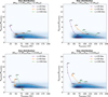 |
Fig. 2 Evolution in the Rgas(90%)/Rdust(90%) vs. Rdust(90%) space for some test substructured disks evolved with DustPy code with external photoevaporation (FFUV = 4 G0) in a low-viscosity regime (α = 10−3.5) for different values of the characteristic radius, rc. The points associated with each trajectory represent the snapshots taken at 0 Myr, 1 Myr, 2 Myr, and 3 Myr, respectively. |
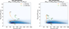 |
Fig. 3 Evolution in the Rgas(90%)/Rdust(90%) vs. Rdust(90%) space for some test substructured disks evolved with DustPy code in a low viscosity regime (α = 10−3.5) for different values of the characteristic radius rc. The points associated with each trajectory represent the snapshots taken at 0 Myr, 1 Myr, 2 Myr, and 3 Myr, respectively. Solid line: External photoevaporation (FFUV = 4 G0). Dashed line: No external photoevaporation (FFUV = 0 G0). |
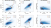 |
Fig. 4 Evolution in the spectral index, size-luminosity, and Rgas(90%)/Rdust(90%) vs. Rdust(90%) spaces of substructured disks evolved with DustPy code with external photoevaporation (FFUV = 4 G0). Low viscosity regime (α = 10−3.5) and disk characteristic radius fixed to rc = 50 au. Different values of the position of the inserted substructure rp are explored. The points associated with each trajectory represent the snapshots taken at 0 Myr, 1 Myr, 2 Myr, and 3 Myr, respectively. Top row: Mdisk = 0.1 Mstar. Bottom row: Mdisk = 0.01 Mstar. |
4 Discussion
4.1 A tension between dust and gas radii
The population study conducted by Delussu et al. (2024) revealed that substructured disks can simultaneously reproduce the observed spectral index and size-luminosity distributions by imposing simple constraints on the parameter space of their initial conditions. However, both the population study performed with two-pop-py (Sect. 3.1) and the study on a test population conducted with DustPy in the presence of external photoevaporation (Sect. 3.2) exposed the difficulty in reproducing the observed ratios of Rgas(90%)/Rdust(90%).
The results obtained from both studies presented in the previous sections demonstrate that both dust sizes and spectral indices can be reproduced if substructures are included. However, in those cases the gas radii are significantly over-predicted. While external photoevaporation can help to shrink the gas sizes, it also ends up limiting the dust disk sizes. In addition, external photoevaporation can even dissipate pressure traps that are near the truncation radius. The results indicate that viscosity works towards increasing the gas size, while radial drift decreases the dust size. Substructures prevent the latter, but an additional mechanism is required to effectively decrease the measured gas size without affecting the dust trapping. Conversely, when gas radii are reproduced, as in Toci et al. (2021) by considering smooth disks, the dust radii end up underestimated.
It is clear that combinations of initial conditions can be found in disks undergoing viscous evolution with external photoevaporation, yielding results that are consistent with observations. However, the limited range of initial conditions required to achieve such outcomes make this a finetuning problem. If measurements of gas radii indeed trace the outer edges of the gas density, while the dust substructure is almost always located within a factor of 2 of this radius, it would suggest either that the outermost trap is somehow associated with the disk truncation radius or that traps are so frequent within each disk that there always exists a trap near the gas outer radius.
In this work, we adopted a constant FUV flux of 4 G0, neglecting the impact of dust extinction and cluster dynamics. Dust can efficiently shield disks from incoming UV radiation in the first 0.5–1 Myr of disk lifetime (see, e.g., Ali & Harries 2019; Qiao et al. 2022). Moreover, the FUV flux experienced by disks is not constant in time due to the relative motion of OBA stars and disks. However, since the Lupus star-forming region does not contain early-type B and O-type stars, we can suppose that this last effect does not substantially compromise our results.
4.2 Possible solutions and future perspectives
Our results show that including external photoevaporation does not fully resolve the discrepancy between the gas-to-dust size ratios of the disks predicted by the models and those observed in the Lupus population. Therefore, it may be necessary to reconsider the assumptions underlying the adopted disk evolution model. We consider whether reducing the α viscosity parameter to lower values (e.g., 10−5) could work to mitigate viscous spreading and lead to the desired outcome. As shown in Delussu et al. (2024) and in Appendix B, assuming such a low viscosity value results in the formation of disks with very low fluxes and overly small rings.
In addition, we considered a constant α value across the disk in this work. However, the dependence of α on the distance from the central star could alter disk’s evolution, including its radius over time. This radius-dependent α profile may, for example, arise due to the presence of dead zones within the disk (e.g., Tong et al. 2024).
Viscous evolution, which leads the disk to spread to larger gas radii, might also be addressed by revisiting our assumption for the initial surface density power law exponent p (Eq. (1)). Indeed, as shown in Toci et al. (2021), p (in their notation γ) has a strong impact on both dust and gas radii. These authors highlight that gas radii are significantly affected by the exact shape of the outer part of the disk which is ultimately determined by p. Lower values of p imply a sharper outer edge, leading to smaller gas radii. Nevertheless, they also show that the effect on dust radii of the choice of p is mitigated after 2–3 Myr due to radial drift. Figure 6 shows that in the case of combined substructures and external photoevaporation, varying p results in evolutionary tracks that rapidly converge towards similar behaviors. This occurs because changing p in the initial gas density profile, but adopting a radially constant α leads to an out-of-equilibrium condition. As a result, disks tend to go back to the p = 1 configuration after a few viscous timescales. However, Fig. 6 shows a promising result as reducing p reduces the initial gas-to-dust size ratio due to the expected reduction in gas radii for p < 1. Appendix C presents the result obtained by combining external photoevaporation and the variation of p with a radially decreasing α profile, which would prevent disks from falling back to the p = 1 scenario. Additionally, this scenario would produce flatter radial profiles of the maximum grain size, in agreement with what was recently observed by multi-wavelength studies (e.g., Sierra et al. 2021; Guidi et al. 2022; Jiang et al. 2024). Nevertheless, the result presented in Appendix C shows disk evolution similar to the case presented in Fig. 6. This is due to the fact that external photoevaporation dominates the shaping of the outer disk region, which ultimately sets the final disk radii. As a result, although the combination of a radially decreasing α and variation in p modifies the overall surface density profile, the impact on the outer disk is effectively erased by external photoevaporation. What remains is a difference in the inner slope, which (as discussed above) does not significantly impact the final disk sizes. This outcome mirrors our previous result when varying only p, confirming that external photoevaporation is the primary driver of disk sizes and confirming that the difference with Toci et al. (2021) arises from the inclusion of external photoevaporation in our model.
An alternative option is to consider a different scenario, where disk evolution is driven by MHD winds. In contrast to purely viscous evolution, where angular momentum is radially transported across the disk, allowing for accretion onto the star, MHD winds extract material (and angular momentum) from the disk. This last mechanism drives disk evolution and accretion without spreading the disk, possibly keeping gas disk sizes small enough to fulfill observational constraints. The discrepancy between the observed and predicted gas and dust disk radii could offer a way to constrain the relative contributions of viscous- and wind-like mechanisms. To compare the two disk evolution frameworks, the implementation of an MHD-wind parametrization (e.g., Tabone et al. 2022) in the numerical codes used is needed and still to be tested.
In this study, substructures have been modeled as gaps associated with the presence of a planet inserted in the disk. These substructures are assumed to be static, and planetary migration is therefore not included. Although a planet-based prescription was adopted, the analysis is not intended to trace the physical origin or evolutionary history of the substructures. Instead, we adopted an agnostic perspective regarding their origin, treating substructures as a generic representation of pressure maxima in disks rather than uniquely ascribing them to migrating planets.
If the substructures considered in this work are interpreted as planet-induced gaps, migration effects may become relevant. However, for the low-viscosity disks and strong dust trapping regimes considered here, gap-opening planets are expected to migrate in the Type II regime, with migration proceeding on the viscous timescale or slower. Under these conditions, the inward displacement of the pressure maximum is expected to remain modest over the disk lifetimes considered and is therefore unlikely to significantly affect the disk radii, which constitute the main observables of this study. A more comprehensive and quantitative assessment of migration effects will be explored in future work.
To further enhance the model’s completeness, we plan to include internal photoevaporation in future work to assess its effects quantitatively. Previous theoretical studies combining internal and external photo-evaporative winds have shown that disks can follow different dispersal pathways depending on the relative strength of these processes, with internal photoevaporation dominating in some regimes and driving inside-out dispersal in others (Coleman & Haworth 2022). For the disk population considered here, internal photoevaporation is expected to primarily affect disks at late evolutionary stages, once accretion rates have dropped to low values. In this regime, its main effect is likely to be the rapid clearing of the remaining gas and the termination of disk evolution, rather than a significant modification of disk structure over megayear timescales. Indeed, external processes, such as external photoevaporation, are expected to dominate the early evolution of large disks (Clarke et al. 2001). A more detailed treatment of internal photoevaporation will be explored in future work.
Neither the stellar luminosity, L⋆, nor the effective temperature, T, were evolved in our simulations. As shown in Delussu et al. (2024), the results obtained when L⋆ (and, thus, T) were allowed to evolve are analogous to those from the fixed-luminosity scenario. Furthermore, while the evolution of stellar luminosity is expected to have a stronger impact for more massive stars (≳1.5 M⊙; e.g., Kunitomo et al. 2021; Ronco et al. 2024), this effect is limited in our study because massive stars do not significantly contribute to our disk population. Indeed, for the two-pop-py simulations, stellar masses have been randomly sampled from the IMF to reflect the distribution observed in star-forming regions; whereas for the DustPy simulations, we adopted two representative stellar masses (0.3 M⊙ and 1 M⊙).
Gravitational instability (GI) can play an important role in massive disks, potentially affecting their structure, dust evolution, and observational signatures at early evolutionary stages. In the disk population adopted in the two-pop-py study, roughly 27% of disks have high disk-to-star mass ratios (Mdisk/Mstar ≥ 0.2), making them potentially prone to GI. Removing this subset produces only modest changes. The mean millimeter continuum flux decreases by approximately 30–40% across the different disk populations, leading to small shifts in the spectral index and size-luminosity distributions. Gas and dust disk radii show an average decrease of less than ~10%, and their distributions remain qualitatively unchanged. Given that gas and dust disk radii are the main observables considered in this study, the inclusion of potentially unstable disks does not affect our population-level conclusions. The effects of GI will be addressed in a follow-up study, where a self-consistent treatment will be implemented.
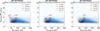 |
Fig. 6 Evolution in the Rgas(90%)/Rdust(90%) vs. Rdust(90%) space of substructured disks evolved with DustPy code with external photoevaporation (FFUV = 4 G0). A low-viscosity regime (α = 10−3.5) is assumed and a disk characteristic radius fixed to rc = 50 au. Different values of the position of the inserted substructure, rp, and the p initial surface density power law exponent values are explored. The points associated with each trajectory represent the snapshots taken at 0 Myr, 1 Myr, 2 Myr, and 3 Myr, respectively. |
5 Conclusions
In this work, we conducted a study to determine whether substructured disks can reproduce the observed gas-to-dust size ratio of the protoplanetary disk population observed in the Lupus star-forming region. Firstly, we performed a population synthesis study of substructured disks using the two-pop-py 1D evolutionary model for dust and gas in protoplanetary disks. Subsequently, we explored the dust-gas size behavior of disks exposed to a moderate environmental FUV radiation field of 4 G0, as the average registered in the Lupus region. The last investigation was performed using the DustPy code extended by an external module that includes the effect of an external FUV field. We compared our simulated disks to the observed dust-gas size distribution of disks of the Lupus star-forming region presented in Sanchis et al. (2021). Our main results are outlined below:
We confirm that smooth disks produce a larger Rgas(90%)/Rdust(90%) compared to observations (Fig. 1), extending Toci et al. (2021) result to the broader level of a disk population synthesis;
We show, on a population synthesis level, as suggested by Toci et al. (2021), that substructured disks (i.e., with one or two substructures) produce lower Rgas(90%)/Rdust(90%), compared to smooth disks (see Fig. 1). However, although the presence of substructures helps mitigate the discrepancy between simulation and observation, it does not completely resolve it;
We identify a tension for substructured disks between the favorable results in Delussu et al. (2024), demonstrating that the spectral index and size-luminosity distributions can be reproduced by simple constraints on their initial conditions, as well as the difficulty in matching the observed gas-to-dust ratios (Fig. 1), even when accounting for external photoevaporation (Figs. 2, 4, and 5);
Specific combinations of initial conditions can produce results consistent with observations for disks undergoing viscous evolution with external photoevaporation (Fig. 4). However, the restricted range of initial conditions required for these outcomes introduces a warning for a fine-tuning problem;
Both population studies exposed the difficulty in reproducing the observed gas-to-dust size ratios. The presence of substructures can reproduce the spectral index and dust size, but leads to an overestimation of the gas radii. On the other hand, when gas radii are reproduced as in Toci et al. (2021), the dust radii end up underestimated. This ultimately emphasizes the fact that the main issue lies in simultaneously reproducing both gas and dust sizes. One possible explanation is that the outermost substructure is linked to the disk truncation radius, which ultimately determines the gas radius; alternatively, it might be the case that substructures are so frequent within each disk that one is always found near the gas outer radius. This could point towards an inability of viscous evolution to reproduce observations if paired with constraints of dust evolution.
In a future work, we aim to extend our investigation by broadening the parameter space of the initial conditions. We will explore further scenarios, such as wind-driven disks, GI, internal photoevaporation, and planetary migration.
Acknowledgements
L.D., T.B., T.C.H.L., and S.M.S. acknowledge funding from the European Union under the European Union’s Horizon Europe Research and Innovation Programme 101124282 (EARLYBIRD) and funding by the Deutsche Forschungsgemeinschaft (DFG, German Research Foundation) under grant 325594231, and Germany’s Excellence Strategy – EXC-2094 – 390783311. G.R. and R.A. acknowledge funding from the Fondazione Cariplo, grant no. 2022-1217, and the European Research Council (ERC) under the European Union’s Horizon Europe Research & Innovation Programme under grant agreement no. 101039651 (DiscEvol). Views and opinions expressed are, however, those of the authors only and do not necessarily reflect those of the European Union or the European Research Council. Neither the European Union nor the granting authority can be held responsible for them.
References
- Adams, F. C., Hollenbach, D., Laughlin, G., & Gorti, U. 2004, ApJ, 611, 360 [NASA ADS] [CrossRef] [Google Scholar]
- Ali, A. A., & Harries, T. J. 2019, MNRAS, 487, 4890 [NASA ADS] [CrossRef] [Google Scholar]
- ALMA Partnership, Brogan, C. L., Pérez, L. M., et al. 2015, ApJ, 808, L3 [Google Scholar]
- Anania, R., Rosotti, G., Gárate, M., et al. 2025a, ApJ, 989, 8 [Google Scholar]
- Anania, R., Winter, A. J., Rosotti, G., et al. 2025b, A&A, 695, A74 [NASA ADS] [CrossRef] [EDP Sciences] [Google Scholar]
- Andrews, S. M., Huang, J., Pérez, L. M., et al. 2018a, ApJ, 869, L41 [Google Scholar]
- Andrews, S. M., Terrell, M., Tripathi, A., et al. 2018b, ApJ, 865, 157 [Google Scholar]
- Ansdell, M., Williams, J. P., van der Marel, N., et al. 2016, ApJ, 828, 46 [Google Scholar]
- Ansdell, M., Williams, J., Trapman, L., et al. 2018, ApJ, 859, 21 [NASA ADS] [CrossRef] [Google Scholar]
- Bae, J., Isella, A., Zhu, Z., et al. 2023, in Astronomical Society of the Pacific Conference Series, 534, Protostars and Planets VII, eds. S. Inutsuka, Y. Aikawa, T. Muto, K. Tomida, & M. Tamura, 423 [Google Scholar]
- Birnstiel, T., Dullemond, C. P., & Brauer, F. 2010a, A&A, 513, A79 [NASA ADS] [CrossRef] [EDP Sciences] [Google Scholar]
- Birnstiel, T., Ricci, L., Trotta, F., et al. 2010b, A&A, 516, L14 [NASA ADS] [CrossRef] [EDP Sciences] [Google Scholar]
- Birnstiel, T., Klahr, H., & Ercolano, B. 2012, A&A, 539, A148 [NASA ADS] [CrossRef] [EDP Sciences] [Google Scholar]
- Birnstiel, T., Andrews, S. M., Pinilla, P., & Kama, M. 2015, ApJ, 813, L14 [NASA ADS] [CrossRef] [Google Scholar]
- Birnstiel, T., Dullemond, C. P., Zhu, Z., et al. 2018, ApJ, 869, L45 [CrossRef] [Google Scholar]
- Bitsch, B., Izidoro, A., Johansen, A., et al. 2019, A&A, 623, A88 [NASA ADS] [CrossRef] [EDP Sciences] [Google Scholar]
- Chambers, J. 2021, ApJ, 914, 102 [NASA ADS] [CrossRef] [Google Scholar]
- Cieza, L. A., Ruíz-Rodríguez, D., Hales, A., et al. 2019, MNRAS, 482, 698 [Google Scholar]
- Cieza, L. A., González-Ruilova, C., Hales, A. S., et al. 2021, MNRAS, 501, 2934 [Google Scholar]
- Clarke, C. J. 2007, MNRAS, 376, 1350 [NASA ADS] [CrossRef] [Google Scholar]
- Coleman, G. A., & Haworth, T. J. 2022, MNRAS, 514, 2315 [NASA ADS] [CrossRef] [Google Scholar]
- Clarke, C., Gendrin, A., & Sotomayor, M. 2001, MNRAS, 328, 485 [NASA ADS] [CrossRef] [Google Scholar]
- Delussu, L., Birnstiel, T., Miotello, A., et al. 2024, A&A, 688, A81 [NASA ADS] [CrossRef] [EDP Sciences] [Google Scholar]
- Drążkowska, J., Alibert, Y., & Moore, B. 2016, A&A, 594, A105 [Google Scholar]
- Facchini, S., Clarke, C. J., & Bisbas, T. G. 2016, MNRAS, 457, 3593 [NASA ADS] [CrossRef] [Google Scholar]
- Gárate, M., Pinilla, P., Haworth, T. J., & Facchini, S. 2024, A&A, 681, A84 [NASA ADS] [CrossRef] [EDP Sciences] [Google Scholar]
- Guidi, G., Isella, A., Testi, L., et al. 2022, A&A, 664, A137 [NASA ADS] [CrossRef] [EDP Sciences] [Google Scholar]
- Guilera, O. M., Sándor, Z., Ronco, M. P., Venturini, J., & Miller Bertolami, M. M. 2020, A&A, 642, A140 [NASA ADS] [CrossRef] [EDP Sciences] [Google Scholar]
- Haworth, T. J., Coleman, G. A. L., Qiao, L., Sellek, A. D., & Askari, K. 2023, MNRAS, 526, 4315 [NASA ADS] [CrossRef] [Google Scholar]
- Huang, J., Andrews, S. M., Dullemond, C. P., et al. 2018, ApJ, 869, L42 [NASA ADS] [CrossRef] [Google Scholar]
- Izquierdo, A. F., Facchini, S., Rosotti, G. P., van Dishoeck, E. F., & Testi, L. 2022, ApJ, 928, 2 [NASA ADS] [CrossRef] [Google Scholar]
- Jiang, H., & Ormel, C. W. 2023, MNRAS, 518, 3877 [Google Scholar]
- Jiang, H., Macías, E., Guerra-Alvarado, O. M., & Carrasco-González, C. 2024, A&A, 682, A32 [NASA ADS] [CrossRef] [EDP Sciences] [Google Scholar]
- Kanagawa, K. D., Muto, T., Tanaka, H., et al. 2016, PASJ, 68, 43 [NASA ADS] [Google Scholar]
- Kenyon, S. J., Yi, I., & Hartmann, L. 1996, ApJ, 462, 439 [NASA ADS] [CrossRef] [Google Scholar]
- Keppler, M., Benisty, M., Müller, A., et al. 2018, A&A, 617, A44 [NASA ADS] [CrossRef] [EDP Sciences] [Google Scholar]
- Kunitomo, M., Ida, S., Takeuchi, T., et al. 2021, ApJ, 909, 109 [NASA ADS] [CrossRef] [Google Scholar]
- Lau, T. C. H., Drążkowska, J., Stammler, S. M., Birnstiel, T., & Dullemond, C. P. 2022, A&A, 668, A170 [NASA ADS] [CrossRef] [EDP Sciences] [Google Scholar]
- Lau, T. C. H., Birnstiel, T., Drążkowska, J., & Stammler, S. M. 2024a, A&A, 688, A22 [NASA ADS] [CrossRef] [EDP Sciences] [Google Scholar]
- Lau, T. C. H., Lee, M. H., Brasser, R., & Matsumura, S. 2024b, A&A, 683, A204 [NASA ADS] [CrossRef] [EDP Sciences] [Google Scholar]
- Lau, T. C. H., Birnstiel, T., Stammler, S. M., & Drążkowska, J. 2025, ApJ, 994, 74 [Google Scholar]
- Lin, D. N., & Papaloizou, J. 1986, ApJ, 309, 846 [NASA ADS] [CrossRef] [Google Scholar]
- Liu, B., Ormel, C. W., & Johansen, A. 2019, A&A, 624, A114 [NASA ADS] [CrossRef] [EDP Sciences] [Google Scholar]
- Long, F., Pinilla, P., Herczeg, G. J., et al. 2018, ApJ, 869, 17 [Google Scholar]
- Long, F., Andrews, S. M., Rosotti, G., et al. 2022, ApJ, 931, 6 [NASA ADS] [CrossRef] [Google Scholar]
- Lüst, R. 1952, Z. Naturforsch. A, 7, 87 [CrossRef] [Google Scholar]
- Lynden-Bell, D., & Pringle, J. E. 1974, MNRAS, 168, 603 [Google Scholar]
- Manara, C. F., Ansdell, M., Rosotti, G. P., et al. 2023, in Astronomical Society of the Pacific Conference Series, 534, Protostars and Planets VII, eds. S. Inutsuka, Y. Aikawa, T. Muto, K. Tomida, & M. Tamura, 539 [Google Scholar]
- Maschberger, T. 2013, MNRAS, 429, 1725 [NASA ADS] [CrossRef] [Google Scholar]
- Matsumura, S., Brasser, R., & Ida, S. 2017, A&A, 607, A67 [NASA ADS] [CrossRef] [EDP Sciences] [Google Scholar]
- Miotello, A., Kamp, I., Birnstiel, T., Cleeves, L., & Kataoka, A. 2023, in Astronomical Society of the Pacific Conference Series, 534, 501 [NASA ADS] [Google Scholar]
- Miyake, K., & Nakagawa, Y. 1993, Icarus, 106, 20 [NASA ADS] [CrossRef] [Google Scholar]
- Morbidelli, A. 2020, A&A, 638, A1 [Google Scholar]
- Müller, A., Keppler, M., Henning, T., et al. 2018, A&A, 617, L2 [Google Scholar]
- Pinilla, P., Birnstiel, T., Ricci, L., et al. 2012, A&A, 538, A114 [NASA ADS] [CrossRef] [EDP Sciences] [Google Scholar]
- Pinilla, P., Birnstiel, T., Benisty, M., et al. 2013, A&A, 554, A95 [NASA ADS] [CrossRef] [EDP Sciences] [Google Scholar]
- Pinte, C., Price, D. J., Ménard, F., et al. 2018, ApJ, 860, L13 [Google Scholar]
- Qiao, L., Haworth, T. J., Sellek, A. D., & Ali, A. A. 2022, MNRAS, 512, 3788 [NASA ADS] [CrossRef] [Google Scholar]
- Ronco, M. P., Schreiber, M. R., Villaver, E., Guilera, O. M., & Bertolami, M. M. 2024, A&A, 682, A155 [NASA ADS] [CrossRef] [EDP Sciences] [Google Scholar]
- Rosotti, G. P., Booth, R. A., Tazzari, M., et al. 2019a, MNRAS, 486, L63 [Google Scholar]
- Rosotti, G. P., Tazzari, M., Booth, R. A., et al. 2019b, MNRAS, 486, 4829 [Google Scholar]
- Sanchis, E., Testi, L., Natta, A., et al. 2020, A&A, 633, A114 [NASA ADS] [CrossRef] [EDP Sciences] [Google Scholar]
- Sanchis, E., Testi, L., Natta, A., et al. 2021, A&A, 649, A19 [NASA ADS] [CrossRef] [EDP Sciences] [Google Scholar]
- Sellek, A. D., Booth, R. A., & Clarke, C. J. 2020, MNRAS, 492, 1279 [NASA ADS] [CrossRef] [Google Scholar]
- Shakura, N. I., & Sunyaev, R. A. 1973, A&A, 24, 337 [NASA ADS] [Google Scholar]
- Sierra, A., Pérez, L. M., Zhang, K., et al. 2021, ApJS, 257, 14 [NASA ADS] [CrossRef] [Google Scholar]
- Stammler, S. M., & Birnstiel, T. 2022, ApJ, 935, 35 [NASA ADS] [CrossRef] [Google Scholar]
- Tabone, B., Rosotti, G. P., Cridland, A. J., Armitage, P. J., & Lodato, G. 2022, MNRAS, 512, 2290 [NASA ADS] [CrossRef] [Google Scholar]
- Takeuchi, T., & Lin, D. 2002, ApJ, 581, 1344 [NASA ADS] [CrossRef] [Google Scholar]
- Takeuchi, T., & Lin, D. 2005, ApJ, 623, 482 [NASA ADS] [CrossRef] [Google Scholar]
- Tazzari, M., Testi, L., Natta, A., et al. 2021b, MNRAS, 506, 5117 [Google Scholar]
- Teague, R., Bae, J., Bergin, E. A., Birnstiel, T., & Foreman-Mackey, D. 2018, ApJ, 860, L12 [NASA ADS] [CrossRef] [Google Scholar]
- Toci, C., Rosotti, G., Lodato, G., Testi, L., & Trapman, L. 2021, MNRAS, 507, 818 [NASA ADS] [CrossRef] [Google Scholar]
- Toci, C., Lodato, G., Livio, F. G., Rosotti, G., & Trapman, L. 2023, MNRAS, 518, L69 [Google Scholar]
- Tong, S., Alexander, R., & Rosotti, G. 2024, MNRAS, 533, 1211 [Google Scholar]
- Trapman, L., Rosotti, G., Bosman, A., Hogerheijde, M., & Van Dishoeck, E. 2020, A&A, 640, A5 [Google Scholar]
- Trapman, L., Tabone, B., Rosotti, G., & Zhang, K. 2022, ApJ, 926, 61 [NASA ADS] [CrossRef] [Google Scholar]
- Trapman, L., Rosotti, G., Zhang, K., & Tabone, B. 2023, ApJ, 954, 41 [NASA ADS] [CrossRef] [Google Scholar]
- Trilling, D., Benz, W., Guillot, T., et al. 1998, ApJ, 500, 428 [Google Scholar]
- Tripathi, A., Andrews, S. M., Birnstiel, T., & Wilner, D. J. 2017, ApJ, 845, 44 [Google Scholar]
- van Terwisga, S. E., & Hacar, A. 2023, A&A, 673, L2 [CrossRef] [EDP Sciences] [Google Scholar]
- Weidenschilling, S. 1977, MNRAS, 180, 57 [NASA ADS] [CrossRef] [Google Scholar]
- Winter, A. J., & Haworth, T. J. 2022, Eur. Phys. J. Plus, 137, 1132 [NASA ADS] [CrossRef] [Google Scholar]
- Woitke, P., Min, M., Pinte, C., et al. 2016, A&A, 586, A103 [NASA ADS] [CrossRef] [EDP Sciences] [Google Scholar]
- Yang, C.-C., Johansen, A., & Carrera, D. 2017, A&A, 606, A80 [NASA ADS] [CrossRef] [EDP Sciences] [Google Scholar]
- Youdin, A. N., & Shu, F. H. 2002, ApJ, 580, 494 [NASA ADS] [CrossRef] [Google Scholar]
- Youdin, A. N., & Lithwick, Y. 2007, Icarus, 192, 588 [NASA ADS] [CrossRef] [Google Scholar]
- Zagaria, F., Rosotti, G. P., Alexander, R. D., & Clarke, C. J. 2023, Eur. Phys. J. Plus, 138, 25 [NASA ADS] [CrossRef] [Google Scholar]
Appendix A DustPy versus two-pop-py
This appendix shows a comparison between DustPy and two-pop-py for substructured test disks. We show the evolution of gas and dust surface densities (Fig. A.1) for a substructured test disk of initial disk mass Mdisk = 0.01 Mstar, initial characteristic radius, rc = 50 au, α = 0.001, vfrag = 1000 cm/s, around a star of mass Mstar = 0.3 Msun, and hosting a planet of mass mp = 1 MJ at rp = 0.5 rc. In Fig. A.2, we show the disk radii, size-luminosity, and spectral index distributions for a population of test disks with initial conditions as listed in the caption of the figure. The models produce similar disk evolution and properties: disk radii and size-luminosity distributions are in good agreement, while modest differences appear near the planet-induced substructure, where two-pop-py produces slightly stronger dust trapping and a sharper pressure maximum. These local variations lead to overlapping but not precisely matching spectral index distributions. However, they do not change the disk radii, which are the main observable considered in this study, and therefore do not affect the gas-to-dust size distributions. Since two-pop-py was not designed or calibrated for substructure, and DustPy includes a more detailed treatment of gap formation, DustPy is adopted for the modeling presented in this study.
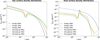 |
Fig. A.1 Comparison of gas surface density (left) and dust surface density (right) evolution between DustPy and two-pop-py models at 0 Myr, 1 Myr, and 3 Myr for a substructured test disk with: α = 0.001, Mstar = 0.3 Msun, Mdisk = 0.01 Mstar, rc = 50 au, vfrag = 1000 cm/s, rp = 0.5 rc, and mp = 1 MJ. |
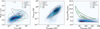 |
Fig. A.2 Spectral index distribution (left), size-luminosity distribution (middle), and gas-dust size distribution (right) comparison between DustPy and two-pop-py at 1 Myr for a test population of substructured disks. Both test populations are constructed by sampling all combinations of the following parameters: α = 0.001, Mstar = [0.3, 1.0] Msun, Mdisk = 0.01 Mstar, rc = [20, 50, 100] au, vfrag = 1000 cm/s, rp = [0.5, 0.7] rc, and mp = 1 MJ. |
Appendix B Low-viscosity case
In this appendix we present the results obtained for a very low α viscosity regime (i.e., α = 10−5), investigating whether reducing the viscosity could help mitigate viscous spreading in the disk. As shown in Delussu et al. (2024) and in Fig. B.1, however, adopting such a low viscosity leads to the formation of disks with very low fluxes and overly small rings, which do not match the observed population.
Appendix C Varying the disk surface density profile and the disk viscosity
Figure C.1 shows the evolution of Rgas/Rdust as a function of Rdust under external photoevaporation, varying the surface density density profile p (Eq. 1), and allowing the α viscosity parameter to decrease with distance to the central star: α = α0(r/rc)−p−1, with α0 = 10−3.5.
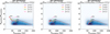 |
Fig. C.1 Evolution in the Rgas(90%)/Rdust(90%) vs. Rdust(90%) space of substructured disks evolved with DustPy code with external photoevaporation (FFUV = 4 G0). Disk characteristic radius fixed to rc = 50 au. Different values of the position of the inserted substructure rp and p initial surface density power law exponent values have been explored. The choice of p is combined with a radially decreasing α profile: α = α0(r/rc)−p−1 with α0 = 10−3.5. The points associated with each trajectory represent the snapshots taken at 0 Myr, 1 Myr, 2 Myr, and 3 Myr, respectively. |
Two-pop-py v1.1.4 was used for the simulations presented in this work.
DustPy v1.0.6 was used for the simulations presented in this work.
All fluxes will be given in frequency space (Fν, typically in units of Jy), even though the subscript is stating the corresponding wavelength instead of the frequency.
All Tables
All Figures
|
Fig. 1 Gas-dust size distribution (first row), spectral index distribution (second row), and size-luminosity distribution (third row) for the parameter space of the initial conditions selecting disks with a spectral index of 0 ≤ α0.89–3.1 mm ≤ 4, 10−3 Jy ≤ F1mm ≤ 10 Jy, 10−3 Jy ≤ F0.89mm ≤ 10 Jy, 100.1 au ≤ Rdust(68%) ≤ 102.6 au, 1 au ≤ Rdust(90%) ≤ 200 au, and 0.1 ≤ Rgas(90%)/Rdust(90%) ≤ 20. Left plots: Smooth disks. Middle plots: Substructured disks with one planet randomly inserted in a range between 0.1–0.4 Myr from the start of the disk evolution. Right plots: substructured disks with two planets randomly inserted in a range between 0.1–0.4 Myr (innermost planet) and between 0.5–0.8 Myr (outermost planet) from the start of the disk evolution. Heatmap of the observed disks with the black dots representing each single observed disk. The black and red lines refer to the simulated results and the observational results, respectively. In particular, the continuous lines encompass 30% of the cumulative sum of the disks produced from the simulations or observed. The dashed lines encompass the 90% instead. |
| In the text | |
|
Fig. 2 Evolution in the Rgas(90%)/Rdust(90%) vs. Rdust(90%) space for some test substructured disks evolved with DustPy code with external photoevaporation (FFUV = 4 G0) in a low-viscosity regime (α = 10−3.5) for different values of the characteristic radius, rc. The points associated with each trajectory represent the snapshots taken at 0 Myr, 1 Myr, 2 Myr, and 3 Myr, respectively. |
| In the text | |
|
Fig. 3 Evolution in the Rgas(90%)/Rdust(90%) vs. Rdust(90%) space for some test substructured disks evolved with DustPy code in a low viscosity regime (α = 10−3.5) for different values of the characteristic radius rc. The points associated with each trajectory represent the snapshots taken at 0 Myr, 1 Myr, 2 Myr, and 3 Myr, respectively. Solid line: External photoevaporation (FFUV = 4 G0). Dashed line: No external photoevaporation (FFUV = 0 G0). |
| In the text | |
|
Fig. 4 Evolution in the spectral index, size-luminosity, and Rgas(90%)/Rdust(90%) vs. Rdust(90%) spaces of substructured disks evolved with DustPy code with external photoevaporation (FFUV = 4 G0). Low viscosity regime (α = 10−3.5) and disk characteristic radius fixed to rc = 50 au. Different values of the position of the inserted substructure rp are explored. The points associated with each trajectory represent the snapshots taken at 0 Myr, 1 Myr, 2 Myr, and 3 Myr, respectively. Top row: Mdisk = 0.1 Mstar. Bottom row: Mdisk = 0.01 Mstar. |
| In the text | |
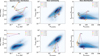 |
Fig. 5 Same as Fig. 4 but for disks with characteristic radius fixed to rc = 100 au. |
| In the text | |
|
Fig. 6 Evolution in the Rgas(90%)/Rdust(90%) vs. Rdust(90%) space of substructured disks evolved with DustPy code with external photoevaporation (FFUV = 4 G0). A low-viscosity regime (α = 10−3.5) is assumed and a disk characteristic radius fixed to rc = 50 au. Different values of the position of the inserted substructure, rp, and the p initial surface density power law exponent values are explored. The points associated with each trajectory represent the snapshots taken at 0 Myr, 1 Myr, 2 Myr, and 3 Myr, respectively. |
| In the text | |
|
Fig. A.1 Comparison of gas surface density (left) and dust surface density (right) evolution between DustPy and two-pop-py models at 0 Myr, 1 Myr, and 3 Myr for a substructured test disk with: α = 0.001, Mstar = 0.3 Msun, Mdisk = 0.01 Mstar, rc = 50 au, vfrag = 1000 cm/s, rp = 0.5 rc, and mp = 1 MJ. |
| In the text | |
|
Fig. A.2 Spectral index distribution (left), size-luminosity distribution (middle), and gas-dust size distribution (right) comparison between DustPy and two-pop-py at 1 Myr for a test population of substructured disks. Both test populations are constructed by sampling all combinations of the following parameters: α = 0.001, Mstar = [0.3, 1.0] Msun, Mdisk = 0.01 Mstar, rc = [20, 50, 100] au, vfrag = 1000 cm/s, rp = [0.5, 0.7] rc, and mp = 1 MJ. |
| In the text | |
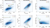 |
Fig. B.1 Same as Fig. 4 but for disks with α = 10−5. |
| In the text | |
|
Fig. C.1 Evolution in the Rgas(90%)/Rdust(90%) vs. Rdust(90%) space of substructured disks evolved with DustPy code with external photoevaporation (FFUV = 4 G0). Disk characteristic radius fixed to rc = 50 au. Different values of the position of the inserted substructure rp and p initial surface density power law exponent values have been explored. The choice of p is combined with a radially decreasing α profile: α = α0(r/rc)−p−1 with α0 = 10−3.5. The points associated with each trajectory represent the snapshots taken at 0 Myr, 1 Myr, 2 Myr, and 3 Myr, respectively. |
| In the text | |
Current usage metrics show cumulative count of Article Views (full-text article views including HTML views, PDF and ePub downloads, according to the available data) and Abstracts Views on Vision4Press platform.
Data correspond to usage on the plateform after 2015. The current usage metrics is available 48-96 hours after online publication and is updated daily on week days.
Initial download of the metrics may take a while.