| Issue |
A&A
Volume 708, April 2026
|
|
|---|---|---|
| Article Number | A28 | |
| Number of page(s) | 14 | |
| Section | Stellar structure and evolution | |
| DOI | https://doi.org/10.1051/0004-6361/202556429 | |
| Published online | 26 March 2026 | |
A search for new symbiotic stars in the Milky Way
Machine-learning techniques applied to photometric databases
1
Departamento de Astronomía, Universidad de La Serena, Raul Bitran, 1720256 La Serena, Chile
2
Instituto de Astronomía y Ciencias Planetarias, Universidad de Atacama, Copayapu 485 Copiapó, Chile
3
Millennium Institute of Astrophysics (MAS), Nuncio Monseñor Sotero Sanz 100, Of. 104 Providencia, Santiago, Chile
4
Department of Physics, University of Rome Tor Vergata, Via della Ricerca Scientifica 1, 00133 Rome, Italy
5
Gemini Observatory/NSF’s NOIRLab, Casilla 603 La Serena, Chile
6
Universidad Nacional de Hurlingham (UNAHUR), Secretaría de Investigación, Av. Gdor. Vergara 2222, Villa Tesei, Buenos Aires, Argentina
7
Consejo Nacional de Investigaciones Científicas y Técnicas (CONICET), Argentina
8
Facultad de Ciencias Exactas, Físicas y Naturales, Universidad Nacional de San Juan, Av. Ignacio de la Roza 590 (O), Complejo Universitario “Islas Malvinas”, Rivadavia J5402DCS, San Juan, Argentina
9
Instituto de Ciencias Astronómicas, de la Tierra y del Espacio (ICATE-CONICET), C.C 467, 5400 San Juan, Argentina
★ Corresponding author: This email address is being protected from spambots. You need JavaScript enabled to view it.
Received:
15
July
2025
Accepted:
9
February
2026
Abstract
Context. Symbiotic stars are interacting binary systems composed of a red giant transferring material to a hot compact star, typically a white dwarf. These systems are crucial for studying stellar evolution, accretion processes, mass transfer, and a variety of complex astrophysical phenomena. However, there is a significant discrepancy between the number of confirmed symbiotic stars (∼ 300) and the estimated population in the Milky Way (1.2 × 10³ − 1.5 × 10⁴), suggesting that a large fraction remains undetected.
Aims. To address this issue, we propose the identification of new symbiotic stars through the application of machine-learning techniques. Our approach combines multiband photometric data from Gaia DR3, 2MASS, and WISE, together with parallax measurements and the pseudo-equivalent width of Hα, to effectively distinguish symbiotic candidates from other stellar populations.
Methods. We trained a random forest model using a sample of 166 confirmed S-type symbiotic stars and a control sample of 1600 nonsymbiotic stars. To mitigate class imbalance and improve the classification performance, we applied the synthetic minority oversampling technique (SMOTE). The model achieved an F1 score of 89% for the symbiotic class.
Results. We applied our model to a catalog of approximately 2.5 million stars selected based on photometric colors consistent with those of S-type symbiotic stars. We identified 990 candidates in this sample with a classification probability of at least 70%. To refine the selection, we applied statistically and physically motivated cuts based on effective temperature, surface gravity, and metallicity and complemented the cuts by SkyMapper photometry. This process yielded 12 high-confidence candidates, characterized by cool temperatures, low surface gravities, solar-like metallicity, Hα emission, luminosities ranging from moderate to high, and ultraviolet excesses consistent with the properties of S-type symbiotic systems.
Conclusions. To evaluate the model performance, we applied it to a validation set of symbiotic stars recently confirmed in the literature. We recovered 92.3% of them. This result supports the effectiveness and generalizability of our classification approach.
Key words: methods: data analysis / astronomical databases: miscellaneous / binaries: symbiotic / Galaxy: stellar content
© The Authors 2026
 Open Access article, published by EDP Sciences, under the terms of the Creative Commons Attribution License (https://creativecommons.org/licenses/by/4.0), which permits unrestricted use, distribution, and reproduction in any medium, provided the original work is properly cited.
This article is published in open access under the Subscribe to Open model. This email address is being protected from spambots. You need JavaScript enabled to view it. to support open access publication.
1. Introduction
Symbiotic stars (hereafter SySts) are long-period interactive binaries composed of an evolved giant star that transfers mass to a hot compact companion, typically a white dwarf (WD), although in rare cases, a neutron star (NS) may be present (see, e.g., Mikołajewska 2012; Munari 2019). These systems are surrounded by a circumbinary nebula formed by colliding stellar winds, photoionization, and collisions (Muerset et al. 1997; Kenny & Taylor 2005; Kilpio & Bisikalo 2009; Mukai et al. 2017). The ongoing interaction between the three components emits across the entire electromagnetic spectrum, from radio wavelengths to X-rays (Luna et al. 2013; Dickey et al. 2021). Each spectral region is dominated by distinct physical components: the cool giant produces absorption features, while the ionized nebula gives rise to prominent emission lines. Furthermore, in approximately 50% of the cases, SySts emit in the O VI lines, which is a unique spectroscopic signature of these systems (Belczyński et al. 2000). Owing to their composite nature, SySts serve as valuable astrophysical laboratories for the study of a wide array of phenomena, including mass accretion, stellar winds, jet formation, thermonuclear outbursts, and stellar evolution (Sokoloski 2003; Mukai et al. 2016). Moreover, they have been proposed as potential progenitors of Type Ia supernovae (Munari & Renzini 1992; Di Stefano 2010; Wang et al. 2010).
According to the evolutionary stage of the cool giant component, symbiotic systems are broadly classified into two subtypes: S-type (stellar) and D-type (dusty) systems (Medina Tanco & Steiner 1995). S-type systems are characterized by their infrared emission, which is dominated by the stellar photosphere of the giant. These systems typically contain red giants with effective temperatures of 3500 to 4000 K, corresponding to spectral types M, K, or occasionally, G (Webster & Allen 1975; Corradi et al. 2003). Their spectral energy distribution (SED) peaks between 1.0 and 1.1 μm, which is consistent with photospheric emission from M3–M6 giants (Ivison et al. 1995; Gromadzki et al. 2007). The cool components are generally located on the red giant branch (RGB) or on the asymptotic giant branch (AGB), and they are photometrically variable due to ellipsoidal modulation, eclipses, or eruptive events (Mürset & Schmid 1999). In contrast, D-type stars are more evolved, often show Mira pulsation, and emit significant warm dust, which shifts the SED to 2–2.5 μm (700–1000K; e.g., Allen 1982; Chen et al. 2019). They sometimes also exhibit two shells with distinct temperatures (e.g., Angeloni et al. 2010). In this case, the spectrum is more similar to that of a planetary nebula than to a giant star. A small group of D-type SySts hosting G- or K-type giants shows even colder dust components. These systems are designated as D’-type and are characterized by peak SEDs at 20–30 μm. In general, the SySt population in the Milky Way are dominated by the S-type (approximately 80%), while the D and D’ types only represent 15% and 3%, respectively.
While the cool component dominates the near-infrared and red optical spectra, the occurrence of symbiotic systems in the shorter wavelengths (ultraviolet, optical, and X-rays) is primarily determined by the hot component. Depending on whether the dwarf is undergoing stable hydrogen-shell burning, SySts systems are classified into shell-burning or accretion-only systems (Sokoloski 2003; Munari 2019). In shell-burning systems, the hot component radiates near the Eddington limit, driving strong photoionization and producing high ionization lines, for example, He II, Fe VII, and O VI (Muerset et al. 1991). These systems are bright in the ultrbands and often exhibit supersoft X-ray luminosities (Luna et al. 2013). On the other hand, accretion-only systems lack continuous nuclear burning and are significantly fainter, with weak or absent emission lines and low ultraviolet and X-ray luminosities. Their discovery usually relies on high-energy observations, as in the case of SU Lyn (Mukai et al. 2016), whose optical spectrum mimics that of a normal red giant star. Recent studies have highlighted the potential of multiwavelength screening techniques for discovering these low-accretion systems. For example, Xu et al. (2024) identified several nearby candidates using ultraviolet and X-ray data combined with European Space Agency’s Gaia Data Release 3 Gaia DR3, suggesting that such accretion-only systems might be more common than previously thought.
Theoretical estimates of the Galactic population of SySts vary significantly, by two to three orders of magnitude, when compared with observational data. The earliest estimate placed the population at ∼4 × 10³ (Kenyon 1986), followed by a substantial increase to ∼3 × 10⁵ by Munari & Renzini (1992) that was later revised to ∼3.3 × 10⁴ by Kenyon et al. (1993), Magrini et al. (2003) proposed a value of ∼4 × 10⁵, assuming that 0.5% of RGB and AGB stars are in binary systems with WDs. The population synthesis models by Lü et al. (2006) suggest a range between 1.2 × 10³. More recently, Laversveiler et al. (2025) estimated lower and upper limits for the SySt population by combining empirical and binary synthesis models, setting the range between 800 and 1400 as a minimum and up to (53 ± 6)×104 as a maximum.
To help close this gap, several authors have used large astronomical databases to identify new candidates. For instance, Corradi et al. (2008) conducted the first systematic search for SySts using narrowband photometric surveys, identifying stars with Hα excess emission in the INT Photometric Hα Survey of the Northern Galactic Plane (IPHAS; Drew et al. (2005)) and infrared excesses based on the Two Micron All Sky Survey (2MASS) photometry, reporting three new discoveries and highlighting the challenge of distinguishing SySts from photometric mimics such as T Tauri and Be stars.
Rodríguez-Flores et al. (2014) reported 14 new SySts using optical photometry from IPHAS and successfully confirmed five new systems, while Li et al. (2015) identified the first halo SySts by cross-matching known systems with spectra from LAMOST DR7, adding a new D-type system from catalogs containing more than four million spectra. Similarly, Akras et al. (2019a) conducted a targeted census of O VI Raman scatterers, discovering 72 new candidate systems, although no new confirmed stars were reported.
The discovery and confirmation of a few hundred new symbiotic stars would place meaningful lower limits on theoretical predictions. However, the relatively low confirmation rates highlight the limitations of traditional identification methods based on individual optical spectroscopic observations, which would have failed in cases such as SU Lyn, whose symbiotic nature became evident only in the high-energy regime. As astronomical databases continue to grow in both size and dimensionality, the manual discovery of rare objects such as SySts becomes increasingly unfeasible. In this context, machine learning (ML) has emerged as a powerful approach for scalable and automated classification in high-dimensional parameter spaces. ML techniques excel at detecting subtle and consistent patterns in complex multidimensional data, thereby improving the identification of the most promising candidates.
Recent studies have begun adopting ML approaches. Akras et al. (2019b, 2021) used decision-tree classifiers to distinguish SySts from Hα-rich mimics; Jia et al. (2023) trained models on infrared photometry from 2MASS and the Wide-field Infrared Survey Explorer (WISE) to classify Large Sky Area Multi-Object Fiber Spectroscopic Telescope sources (LAMOST Cui et al. 2012), confirming two new SySts; and Ball et al. (2025) developed a Gaia-only pipeline integrating photometry, astrometry, and compressed XP spectra to identify more than 1600 new candidates.
Despite the growing application of ML in identifying rare astrophysical objects, recent reviews (Merc 2025) have highlighted persistent structural limitations in current pipelines. First, there is a noticeable lack of standardized training datasets: many models are trained on heterogeneous photometric catalogs without common calibration or physical priors. Second, typical ML classifiers often depend on infrared-only photometric bands, which limits their ability to generalize across different SySt subtypes. For example, Jia et al. (2023) presented more than 10 000 candidates using 2MASS and WISE photometry, but only two objects were spectroscopically confirmed. This highlights the need for a more physically informed ML approach, in which constraints from domain knowledge are incorporated to narrow the candidate-selection space more effectively.
We developed a supervised ML framework to identify new candidates for S-type SySts. Our decision to focus exclusively on S-type systems was motivated by physical, methodological, and computational considerations. In addition to constituting the majority of the known Galactic population, these systems exhibit more uniform photometric properties, which facilitates their characterization and distinction from other stellar types.
Our approach leveraged a combination of astrometric and photometric data from Gaia, 2MASS, and WISE, constrained within an observationally defined parameter space and specifically tailored to the characteristics of S-type SySt systems. The main goals of this work are to identify previously unknown S-type candidates and to assess the reliability of previously proposed systems using classification models trained with characterized color indices. The structure of the paper is as follows: Section 2 describes the dataset construction and selected features. Section 3 describes the ML method. Section 4 presents the model performance metrics. Section 5 applies the trained model to the full dataset and highlights the most promising candidates. Section 6 compares our results with those of previous approaches, and Sect. 7 concludes with the implications of our findings.
2. Data
For this study, we adopted as a reference the New Online Database of Symbiotic Variables (hereafter Merc’s catalog, Merc et al. 2019)1, which constitutes the most comprehensive compilation to date of spectroscopically confirmed symbiotic systems, both in the Galaxy and in nearby extragalactic environments. In particular, this catalog contains information about 1190 sources in the Milky Way, of which 284 are confirmed (203 S-type and 39 D-type), 690 are suspected, 78 are possible, 46 are likely and 155 are misclassified. For the definition of each category, we refer the reader to Merc (2022).
This catalog provides uniform and referenced data on observational parameters (e.g., positions and multiband photometry), as well as physical characteristics, including orbital elements, component properties and subclassifications. In addition to infrared measurements, the database integrates multiwavelength information from X-ray missions such as ROSAT and Swift (Evans et al. 2020; Boller et al. 2016, respectively), along with astrometric and photometric data from the Gaia mission. For the purposes of this work, we restricted our sample to confirmed Galactic systems to select the photometric databases used for training ML model.
The selection was guided by the completeness of photometric data available for each object, as shown in Fig. 1. Among the databases considered, the ones offering the most complete coverage were Gaia DR3 (Gaia Collaboration 2016, 2023), the Two Micron All Sky Survey (2MASS; Skrutskie et al. 2006), and the Wide-field Infrared Survey Explorer (WISE; Wright et al. 2010). While all four WISE bands were initially retrieved, only W1 (3.4 μm, Δλ = 0.66 μm) and W2 (4.6 μm, Δλ = 1.04 μm) were retained for this study, as they provide an optimal trade-off between sensitivity and spatial resolution, which is essential for the ML model developed. At these last wavelengths, the infrared emission of SySts is typically dominated by the Rayleigh-Jeans tail of the giant continuum, modulated by the absorption features such as CO and H2O bands. Therefore, W1 and W2 trace the photospheric emission of the cool giant, allowing for an effective separation between the S-type, which is characterized by a stellar continuum with very little dust contribution, and D-type systems.
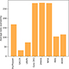 |
Fig. 1. Average number of valid measurements per photometric group in the sample. Each bar represents the mean number of available (not missing) values for the bands belonging to a given instrument or spectral range. |
It is also important to note that fundamental stellar parameters from Gaia, such as effective temperature (Teff), surface gravity (log g), and metallicity ([Fe/H]), were excluded from the training set, since these quantities are available for only about 50% of confirmed SySts. Given the limited number of objects with complete measurements, we chose not to apply data-imputation techniques, as this would not be statistically robust.
Then, photometric colors were obtained by combining bands from the same study to minimize the effects of intrinsic variability. Although the observations are not strictly contemporaneous, this does not significantly affect the derived colors: the typical timescales of variability in SySts, such as pulsations and orbital modulations, are larger than the time separations between bands in surveys such as Gaia, 2MASS, and WISE. Therefore, while the intrinsic variability remains a relevant factor, the impact of the color measurement is expected to be limited in the context of population level classification.
In this study, we limited our analysis to S-type SySts. This decision is based on the distinct photometric behavior of the different subclasses. D and D’ type systems possess extended dusty envelopes that significantly affect their infrared emission, especially, beyond 2 μm. These dusty components contribute to strong mid-infrared excess, which shifts their colors away from the photospheric sequence defined by the dusty-free systems. As a result, these objects occupy a broader and more dispersed region in the color-color diagrams shown in Fig. 2, making it difficult to define a consistent photometric locus suitable for supervised classification.
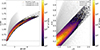 |
Fig. 2. Color–color selection process. Left: 2D histogram of approximately 17 988 392 sources obtained from four ADQL queries to the Gaia services and a WISE cross-match. The first selection cut was applied in the Gaia color–color diagram using a linear regression in logarithmic scale, resulting in the removal of 143 434 sources. Confirmed SySts are marked as orange stars. Right: 2D histogram of over 4 million sources selected from the 2MASS color–color diagram. The color bar indicates the number of sources per bin in logarithmic scale for both panels. |
From this reference sample, we determined the minimum and maximum values for each color index (see Table 1), defining a multidimensional color space representative of S-type SySts. These bounds were subsequently used to retrieve photometrically similar sources from the Gaia DR3 extended dataset. Furthermore, we adopted the observed range of pseudo-equivalent width Hα (EWHα), obtained from the Gaia DR3 astrophysical_parameters table. These values are calculated from low-resolution XP spectra evaluated between 646 and 670 nm, and span from 0.69 Å to −18.49 Å (negative values indicate emission). Parallax values between 0 and 5.29 mas were also used as an empirical constraint to restrict the search space. These criteria were designed to favor the identification of sources with properties consistent with those of confirmed S-type SySts.
Color limits in the ADQL query.
The photometric, spectroscopic, and astrometric limits defined above are critical to ensuring the quality and reliability of the training dataset used for the ML model. The Merc catalog includes a wide variety of SySts candidates and confirmed systems, compiled from heterogeneous sources, which may differ in classification criteria and observational coverage. Incorporating all available data without extensive validation could introduce inconsistencies and biases that impair model performance. Therefore, we limited our selection to confirmed S-type systems with well-characterized photometric, spectroscopic, and astrometric measurements. This approach prioritizes uniformity and robustness over sample size, allowing the model to learn from a representative and reliable dataset that reflects properties of S-type SySts.
After this, we performed an ADQL query using Gaia DR3 services to identify sources that matched the characteristic color ranges of S-type SySts (see Table 1). To ensure the reliability and relevance of the selected data, several additional criteria were applied. First, we restricted the sample to sources with magnitudes in the G band brighter than magnitude 16, a range in which Gaia provides higher precision astrometric and astrophysical parameters according to Anders et al. (2019). Second, we selected only those sources with parallax measurements and EWHα values available and within the range described above. To further ensure high-confidence distance estimates, we required a parallax signal-to-noise ratio greater than 10, a threshold commonly adopted in Gaia-based studies (e.g., Lindegren et al. 2020). Finally, we required all selected sources to include a reliable counterpart in the 2MASS catalog, using the ESA-provided cross-comparison table gaiadr3.tmass_psc_xsc_best_neighbor, to ensure consistent photometric information across all surveys.
To optimize the information without overloading the Gaia search services, the ADQL query was divided into four sky regions, each spanning a 45° declination range and covering the full 24 hours of right ascension. A simplified version of this query can be found in Appendix A. The query yielded approximately 18 million records, representing only 1% of the Gaia DR3 data. These results were compared to the WISE catalog using the TOPCAT tool (Taylor 2005), with a tolerance of two arcsec. To ensure that no source is repeated in this catalog, an internal cross-match of the catalog was performed with a tolerance of 5 arcsec, from which one star was excluded. This catalog, with 17 988 392 sources, is represented in the right panel of Fig. 2 by the gray background.
With this, we start the data curation process. First, we excluded from this catalog the known SySts and restricted the W1−W2 color to −2.79 and 1.93, which corresponds to the same color range of S-type SySts. Subsequently, we constructed color-color diagrams using Gaia photometry, where it was observed that this type of stars is concentrated in a specific region of the plane. To define it, a linear regression was used with the vertical axis in logarithmic scale, from which the equation
 (1)
(1)
was obtained. From Eq. (1), a lower and upper limit were defined, which is represented in the right panel of Fig. 2 by the dashed lines in both panels using a 1σ difference defined by visual inspection (σ = 0.24). This same procedure was applied to the 2MASS color plane using the selected data shown in the left panel of Fig. 2. The linear regression results in Eq. (2),
 (2)
(2)
In this process, equations for the upper and lower bounds were defined using a 2σ envelope (σ = 0.15) by visual inspection. These equations are described at the top of right panels of Fig. 2. After applying the color–color selection criteria described in the same figure, the filtered catalog retained approximately four million sources. Subsequently, we applied the data-cleaning procedure described by Monsalves et al. (under review), which consists of excluding the 1% of outliers in the distribution of relevant features, photometric colors, EWHα The analytical expressions for the boundaries are shown at the top of the left panel in Fig. 2.
This procedure further reduced the sample to approximately 2 540 539 objects photometrically similar to SySts. Application of the same selection and cleaning criteria to the initial set of S-type SySts from the Merc catalog reduced the sample from approximately 203 to 166 stars. This careful filtering ensured the homogeneity and reliability of the reference sample we used to train the ML model. Importantly, the photometric data used in this study were neither dereddened nor corrected for interstellar extinction. However, since the most distant sources in the sample are located at approximately 6 kpc, the effect of extinction is expected to be modest and to not significantly affect the classification based on observed colors. Furthermore, this approach agrees with the intended application of the model to observed survey data, which are also uncorrected.
3. Searching for SySts: ML approach
3.1. Training, test, and validation sets
To build the training and test sets, we cross-matched the point source subcatalog with the SIMBAD database (Wenger et al. 2000), using the position with a tolerance of two arcseconds and considering the main_type field. This yielded ∼304 230 sources with known classifications, including various types of variable stars (e.g., Mira, Cepheids, and long-period variable stars), evolved stars (e.g., AGB, RGB, red supergiants, and Wolf–Rayet stars), young stellar objects (e.g., T-Tauri and Herbig Ae/Be), and other peculiar Galactic sources. Many of these classes are known photometric mimics of S-type SySts in color-color space (Corradi et al. 2008; Akras et al. 2019b).
To define the negative class for the binary classifier, we first removed sources with ambiguous or uncertain types (e.g., LPV_Candidate or LPV*), reducing the initial sample by about half. From the remaining labeled sources, we constructed the training subset by progressively subsampling the negative while enforcing statistical consistency with the parent distribution. Specifically, for all features used in the classifier (Gaia, 2MASS, and WISE colors, parallax, and Hα indices), we performed two-sample Kolmogorov–Smirnov tests (Kolmogorov 1933; Smirnov 1948) comparing each candidate subsample against the full negative population. Subsamples were iteratively reduced until every feature satisfied a p-value threshold of > 0.05, ensuring that their marginal distributions remained statistically indistinguishable from those of the complete set (see Appendix B for the full list of KS statistics and p-values). The final subset of 1600 sources consists primarily of objects labeled as Star (1580), along with a small number of EclBin (12), RSG (2), YSO (2), and one each of far-infrared and infraredsources, thus preserving the heterogeneity of the negative class.
To this negative class, we added 166 confirmed S-type SySts from Merc’s catalog, which constitute the positive class. The full dataset was split using an 80:20 ratio, resulting in 133 S-type SySts and 1279 negative-class objects for training, and 33 SySts and 320 negative-class objects for testing, respectively. All preprocessing and data balancing steps described below were applied exclusively to the training subset, after the 80:20 split. The test partition remained untouched throughout training, calibration, and evaluation, ensuring a leakage-free workflow. The distribution of both classes is shown in Fig. 3.
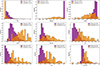 |
Fig. 3. Distribution of the training set characteristics for the positive class (S-type SySts) and the negative class (“others”). |
In addition to these samples, we took an independent validation sample composed of recently confirmed symbiotic S-type stars. These sources are not included in the Merc catalog, as they were identified more recently. However, their symbiotic nature has been confirmed spectroscopically, providing a reliable and unbiased benchmark for evaluating model performance in real, never before observed cases. This validation sample builds on the work of Lucy et al. (2025), who proposed a novel photometric selection technique using SkyMapper Southern Survey (SkyMapper Bessell et al. 2011) photometry, specifically in the u, v, and g bands. Their method focused on identifying outliers in u-band photometry, particularly those exhibiting significant excess ultraviolet and infrared signatures consistent with S-type SySts. This approach effectively highlights systems with anomalous photometric behavior, which are often associated with symbiotic interactions. From their list, we used the 12 spectroscopically confirmed sources, ensuring that they were compatible with the previously defined parameter space for the classifier. By ensuring compatibility with the original feature distributions, this selection enables a robust and meaningful assessment of the of the model generalization capability. Notably, none of these sources were included in the training or testing phases. Their inclusion as an external validation set allowed us to test the predictive accuracy of the classifier under realistic conditions, using independently identified systems that are representative of the target class, but without training bias.
As a complement, a second validation set was incorporated, consisting of photometric impostors included in the Merc catalog as misclassifications. These correspond to objects that were initially reported in the literature as possible SySts but were later reclassified after spectroscopic confirmation. The original set comprises 155 sources distributed across the Milky Way; however, only 90 meet the consistency criteria within the adopted parameter space. These sources encompass a wide variety of stellar types that are often photometrically confused with SySts, such as variable stars, massive stars and supergiants, planetary nebulae, cataclysmic variables, subdwarfs, and young stellar objects. The inclusion of this group allows us to explore the limits of photometric separability between genuine SySts and their main contaminants that have been observationally identified.
3.2. Data-balancing algorithm
The training subdataset consisted of 1279 sources from the negative class and only 133 confirmed S-type SySts from the positive class, resulting in a significant imbalance with a ratio close to 90:10. To address this problem, we applied the Synthetic Minority Oversampling Technique (SMOTE, Chawla et al. 2002), an algorithm widely used to address class imbalance in classification problems. SMOTE creates new synthetic examples of the minority class, generating interpolations between each object and its nearest neighbors in the feature space defined for the classifier. This approach expands the minority class while preserving the structure of the original data.
SMOTE was applied to the training subset after the 80:20 split, while the test and validation sets remained untouched during the analysis. This resulted in a balanced dataset. The effectiveness of SMOTE in astronomical applications has been demonstrated in several recent works addressing highly unbalanced datasets. Some examples are Chen et al. (2004), Hosenie et al. (2020), Maravelias et al. (2022), Avdeeva (2023).
3.3. Random forest model
We employed a random forest (RF) binary classifier (Breiman 2001), implemented using the Python library (imblearn; Lemaître et al. 2017), to distinguish candidates of S-type SySts from photometric mimics. RF is a supervised ensemble learning method that builds a collection of decision trees, each trained on bootstrap samples of the original dataset. At each node, a random subset of features is considered, introducing diversity among the trees and reducing their correlation. This ensemble strategy lowers the variance of the model and mitigates the overfitting typically observed in individual decision trees, enhancing its generalization capacity in complex classification tasks involving correlated astrophysical parameters.
The model was trained using nine input features that combine photometric and astrometric information: seven color indices derived from Gaia, 2MASS, and WISE, the (EWHα), and parallax. Hyperparameter tuning was performed via exhaustive grid search with 5-fold cross-validation using GridSearchCV (Buitinck et al. 2013), applied to the training subset, leading to a final configuration with 800 trees, a minimum of ten samples to split a node, two samples per leaf, and log2 of the total number of features considered at each split and a maximum depth of 10 was imposed, allowing the trees to grow sufficiently deep to capture complex nonlinear patterns. This setup enables the model to effectively learn the intricate feature interactions and distributions characteristic of astrophysical data, yielding a robust and reliable classifier for the identification of S-type SySts candidates within large and heterogeneous samples.
4. Results
To evaluate the performance of the RF Classifier, we employed four widely recognized metrics: precision, recall, F1 score, and PR-AUC (Powers 2011). These metrics provide a comprehensive assessment of the model’s predictive capabilities, focusing on different aspects of classification performance.
Precision quantifies the ability to minimize false positives, recall measures the model capacity to identify true positives, and the F1 score balances precision and recall to offer a single performance measure. Finally, the PR-AUC summarizes the classifier performance across varying classification thresholds.
Table 2 summarizes the RF model classification performance, evaluated via repeated stratified 5-fold cross-validation (3 repetitions). The classifier achieves near-perfect scores for the negative class (“Others”) and robust results for the symbiotic class, with 93% precision, 85% recall, and an F1 score of 89%. The slightly lower recall reflects the inherent class imbalance, but overall the model reliably distinguishes SySts. Furthermore, the analysis of error rates as a function of the classification threshold shows that the false positive rate decreases from 0.6% to 0.3% when increasing the decision boundary from 0.5 to 0.7, while the false negative rate rises from 15.2% to 27.3%. These trends indicate that stricter thresholds substantially reduce contamination at the cost of a moderate loss in completeness.
Performance scores per class for the RF classifier applied to the test sample with their respective standard deviation.
To reduce FP contamination and increase confidence in candidate identification, we enforce a stricter classification threshold of 70%. This setting prioritizes precision over recall, which is especially relevant for underrepresented classes like SySts and allows for a compromise between data quantity and data quality. The confusion matrix in Fig. 4 illustrates the classification performance on the test set, composed by a 20% of the training catalogs, which consists of 321 objects from the negative class and 33 from the positive class (SySts).
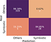 |
Fig. 4. Confusion matrix for the testing set using SMOTE + RF, incorporating photometric colors, parallax, and EWHα. The x-axis represents the predicted class (predicted label), and the y-axis denotes the actual class (true label). Each cell shows the percentage relative to its respective class on the first line, followed by the corresponding number of stars on the second line. |
The model correctly identifies 319 out of 321 nonsymbiotic sources based on their stellar parameter estimates. Only two FPs were found, corresponding to an eclipsing binary and a young stellar object. Additionally, five FNs were identified: four of them are accretion-only SySts, one of which contains an NS companion, and the remaining case is a shell-burning system characterized by strong Raman emission. The results highlight the conservative nature of classifier, which prioritized a low FP rate, an essential criterion for effective spectroscopic follow-up, particularity in the context of rare-objects search. Unlike previous studies that presented a large number of candidates (several hundred thousand), often with limited reliability, our approach emphasizes precision over quantities. In practice, the utility of a large sample of candidates is significantly reduced if it includes a substantial number of FPs because a spectroscopic confirmation of all these candidates is highly unlikely. A model that minimized the probability of contamination is therefore more valuable, even at the expense of completeness. The small but highly reliable sample produced by our classifier offers a more efficient path toward confirmation, maximizing the scientific return of follow-up observations. The low number of FPs demonstrates the model robustness in separating genuine symbiotic systems from photometric mimics, while the few FNs reflect the intrinsic heterogeneity and observational diversity within the SySts class.
To assess the relevance of the input features in the classification process, we evaluated the feature importance using two complementary approaches: the RF mean decrease in impurity (MDI), and the permutation feature importance, the latter computed as the decrease in the F1 score after randomly shuffling the values of each feature. Figure 5 directly compares these two estimators of the global feature importance.
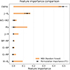 |
Fig. 5. Comparison between the mean impurity decay of random forest (MDI, orange bars) and the importance of permutation features calculated using the F1 score (black dots). |
Despite their different conceptual definitions, both methods consistently identify the EWHα as the most influential feature of the model. This result is entirely consistent with the spectroscopic properties of the S-type SySts used in this work, as approximately 95% of the confirmed systems exhibit Hα in emission. A detailed discussion of the role of Hα is provided in Sect. 5.2.
After Hα, the J–Ks near infrared color emerges as the second most relevant feature in both importance estimators. This color traces the photospheric emission of the cool giant component, whose spectral energy distribution peaks in the near-infrared (0.8-1.1 μm), as expected for late-type giants.
Beyond the J−Ks color, the relative importance of the remaining features is less clearly ordered. The two estimators no longer show a strict one-to-one correspondence in their ranking, and several parameters, including additional near-infrared colors, optical color indices, and parallax, display comparable importance values. This behaviour indicates that, at this level, the classifier exploits a combination of correlated observables rather than relying on a single dominant parameter.
In particular, the contribution of parallax should not be interpreted as a direct physical diagnostic. In long-period binary systems such as S-type SySts, unresolved orbital motion can introduce systematic biases in Gaia astrometric solutions. While a parallax threshold was applied to ensure basic astrometric reliability, its role in the model likely reflects indirect correlations with distance-dependent photometric quantities rather than intrinsic physical information.
At the other end of the ranking, features with the lowest importance correspond to Gaia optical color indices (G−BP, BP−RP). Owing to the extremely broad Gaia passbands, spanning from the near-ultraviolet to the near-infrared (∼300–1000 nm), these colors tend to dilute narrow but intense emission lines such as Hβ, [O,III], and Hα, thereby reducing their discriminating power relative to infrared indices.
In addition, we evaluated the performance of the model using a validation set composed of 12 confirmed S-type SySts taken from Lucy et al. (2025). All of these stars are within the parameter range in which the model was trained, which ensured that the validation set agreed with the characteristics of the dataset used in the training. As a result of this evaluation, the model was able to correctly recover 11 of the 12 SySts, implying a detection rate of 92.3%. All recovered stars exceeded the previously proposed classification threshold of 70%. The average probability of symbiotic class membership for these stars was 97%, with a standard deviation of only 0.05%, reflecting consistency in the model predictions.
The only unrecovered source from the validation set was the variable star V V1918 Sgr*, a binary system previously classified in the literature as a planetary nebula, whose cool component was identified as a K4 I supergiant. This classification is consistent with its extreme W1–W2 color, which placed the object at the edge of the parameter space covered by our training sample. Although its photometric parameters formally lie within the model training domain, several of its features are sparsely represented in the training set. A local SHAP (Lundberg & Lee 2017) analysis of this source (Appendix C) indicated that its classification is affected by a combination of photometric and spectroscopic features, including the EWHα, and by the optical (G–BP) and infrared (W1–W2) colors. In particular, the Hα values dominate the shift of the prediction below the symbiotic classification threshold, while W1–W2 and G–BP provide a secondary contribution to the final decision.
This case illustrates a limitation of the model when it is applied to objects with atypical stellar components, and it suggests that its performance might degrade for systems that are dominated by very luminous or otherwise peculiar donors, in which spectroscopic indicators such as Hα might no longer play a dominant role, while broadband optical and infrared colors become the primary drivers of the classification. These regimes are underrepresented in the training data.
To further evaluate the model robustness, we additionally tested the classifier using a validation set of 155 photometric mimics, of which 90 lie within our parameter space (i.e., misclassifications reported in the Merc et al. 2019 catalog). These sources were initially proposed as possible SySts but were later spectroscopically rejected. The test resulted in 51 objects being incorrectly classified as symbiotic, increasing the model contamination rate from 15.15% to approximately 33.35%. Among the contaminants, we identified 12 massive and supergiant stars, 10 planetary nebulae, 9 variable stars, 6 evolved giant stars, 5 young stellar objects, 4 subdwarfs, and 4 eclipsing binaries.
5. Complementary analysis of SySt candidates
After validating the model performance, we applied it to a filtered dataset of 2 538 939 objects, as described in Sect. 2, excluding the stars used in the training sets. This process yielded a total of 1,559 candidate S-type SySts with probabilities higher than 50%, from which we recovered 990 with probabilities exceeding 70%. We then performed a preliminary analysis of these sources using Gaia DR3 data – specifically the mh_gspphot module (Recio-Blanco et al. 2023) – and SkyMapper DR2 (Onken et al. 2019) photometry, with the aim of extracting key astrophysical and photometric parameters such as luminosity, Teff, [Fe/H], log g, and EWHα.
The Galactic distribution of the confirmed S-type SySts and the candidates identified in this work is shown in Fig. 6, where the dashed lines mark the region |b|< 15°, commonly associated with a higher density of SySts in the Milky Way (Merc et al. 2021). However, this apparent concentration toward the Galactic plane may be partly driven by selection effects, as large-scale surveys often focus on the disk. Previous studies, such as Munari & Dallaporta (2021), have shown that SySts can also be found at higher Galactic latitudes, suggesting that the observed distribution may not fully reflect the intrinsic spatial population of these systems.
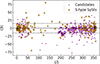 |
Fig. 6. Galactic distribution of 990 SySt candidates (purple points) according to our model and confirmed S-type of SySts (orange stars). |
5.1. Physical parameters from Gaia
Astrophysical parameters for the 990 candidates were retrieved using the Gaia DR3 mh_gspphot module, subject to data availability. While these parameters offer valuable complementary diagnostics for candidate characterization, they must be interpreted cautiously. The atmospheric models used for parameter estimation (Creevey et al. 2023) are not optimized for complex systems like SySts, which often exhibit variability and binary interaction effects.
Luminosities were estimated via absolute magnitude in the G band (MG), calculated from apparent magnitudes, parallaxes, and extinction corrections. Extinction (AG) was derived from reddening maps by Schlegel et al. (1998), accessed through the dustmaps package (Green et al. 2024). To assess evolutionary stages, candidates were classified based MG: those with MG < −0.5 were considered likely AGB stars, while sources with −0.5 ≤ MG ≤ 2.5 were classified as RG. Approximately 67.3% of objects with valid luminosities fall in the AGB regime and 8.6% in the RGB regime, consistent with evolved giant stars.
The Teff mostly lie within 3500–4000 K, typical of M-type giants. However, about 15% of candidates show higher values around 15 000 K, which are too low to represent the hot white dwarf components (usually 50 000–150 000 K). These intermediate temperatures likely arise from composite spectra where the hot component, accretion disk, and nebular emission contribute to the optical flux, as observed in systems like T CrB and CH Cyg (Zamanov et al. 2015; Stoyanov et al. 2018). This complexity challenges the applicability of single-star atmospheric models.
The [Fe/H] spans from −4.1 to +0.8, reflecting the chemical diversity expected across the Galaxy. Since SySts originate in varied galactic environments, this wide range, including solar and subsolar values, is consistent with confirmed samples, and thus not a strong membership discriminator.
The log g values from Gaia range between –0.1 and 4.7, differing from the typical −1 to 1 expected for S-type SySts (Gałan et al. 2017, 2023). Only 674 candidates fell within the expected range. This discrepancy likely stems from the intrinsic complexity of SySts, such as binarity, variability, and composite spectra, which limit the reliability of Gaia’s single star models. Therefore, log g should be interpreted with caution and in conjunction with other parameters.
Importantly, none of these astrophysical parameters were used to exclude candidates. Sources lacking reliable Gaia estimates or falling outside expected ranges remained in the sample. Instead, this information helped us to prioritize targets for followup and to focus on those whose physical properties match those of confirmed SySts best.
5.2. Hα emission
The values of EWHα in the candidates sample exhibit values ranging from −10.6 to −0.6 Å, with a median around −0.8 Å. This confirms the presence of Hα emission in all sources, although generally weaker than in the confirmed sample of S-type SySts, which has a median EWHα of −4.2 Å. This difference may reflect intrinsic variability or accretion-only states of the stars, or the inclusion of false positives, which according to the confusion matrix should occur in about 15% to 33% of the data.
Nevertheless, the EWHα values employed here correspond to the Gaia DR3 pseudo-equivalent widths, which are derived from low-resolution BP/RP spectra and rely on automated continuum estimation. As discussed by Creevey et al. (2023), a temperature-dependent correction is applied for sources cooler than Teff < 5000 K, which may not be fully adequate for the cool giant components typical of symbiotic systems. Furthermore, Shridharan et al. (2022) found that Gaia’s EW values can be systematically biased for emission-line stars due to the simplified background model adopted in the pipeline. These effects could lead to either an underestimation or overestimation of the actual emission strength, especially in composite or dust-affected spectra. Therefore, while the Gaia Hα emerges as the most relevant feature in the MDI and permutation analyses (Sect. 4), its absolute values should be interpreted with caution, and future higher-resolution spectroscopy will be necessary to validate these measurements.
5.3. SkyMapper photometry
We performed a cross-compatibility test on our candidates with SkyMapper DR2 to study their photometric behavior in the ultraviolet regime. Of the 990 candidates, 660 presented valid u, v, and g photometries, as shown in Fig. 7. Following Lucy et al. (2025)’s criteria, we selected sources with u < 16 mag and u − g < 2.4, indicative of a hot, compact companion. A total of 145 candidates met these conditions.
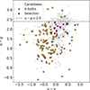 |
Fig. 7. Color-color plot of the SkyMapper u − v vs. u − g photometry for our candidates (gray dots), known SySts (orange dots), and the 12 most likely candidates (purple dots). |
Figure 7 presents the u − v versus u − g color-color plot, where the gray dots represent the full candidate sample and the orange symbol corresponds to the known SySts. These color indices effectively isolate symbiotic systems: u − g is sensitive to the ultraviolet excess of the hot component, while u − v provides an orthogonal axis that helps distinguish different stellar populations (Lucy et al. 2025).
Most of the known SySts cluster in the lower left region, reflecting a strong ultraviolet excess, consistent with an active hot companion. A more dispersed group appears towards higher u − g values, corresponding to systems with disk activity or nova-like eruptions, where the ultraviolet colors vary due to accretion changes or dimming. This color-space therefore serves as a powerful diagnostic tool for the photometric identification of SySts, capturing both classical hot systems and more complex or evolved objects with variable activity.
5.4. Refined candidate selection
To isolate the most promising candidates, we applied a multiparameter filtering approach based on the criteria summarized in Table 3. These included astrophysical parameters derived from Gaia described above, such as Teff, MG, log g, and [Fe/H], as well as constraints on ultraviolet excess indicators obtained using SkyMapper photometry.
Selection criteria used to refine the candidate sample.
The adopted thresholds were defined by combining two strategies: statistical cutoffs based on the distribution of confirmed S-type SySts, typically using the median value ±3σ, and empirical limits reported in the literature, particularly in the case of SkyMapper colors. This approach ensured that the selected subsample occupies a parameter space consistent with known interacting binaries, while allowing for physical diversity. After applying these filters to the full set of 990 high-confidence candidates, we identified a refined sample of 52 sources whose physical and photometric properties closely resemble those of confirmed S-type SySts. Among these, 12 objects also exhibit significant ultraviolet excess, as defined by our SkyMapper criteria, reinforcing their classification as likely systems interacting with a hot component. Table 4 lists the main parameters of these 12 high-priority candidates, represented by purple dots in Fig. 7. It is important to emphasize that the strict selection applied here is intended to prioritize targets for immediate spectroscopic follow-up.
Candidate SySts based on Gaia DR3 parameters.
6. Comparison with previous works
Our study focuses on the identification of new SySt candidates through ML techniques applied to public datasets. While previous works have employed similar approaches, our method stands out by utilizing the largest available catalog of point sources to date, along with the integration of low-resolution astrometric and spectroscopic data.
To validate and contextualize our classification results, we compared them against five previously published catalogs selected based on their similarity in feature sets used for training and classification. This comparison includes the total number of sources in each catalog, the subset within the defined parameter space of our model, and the fraction of sources classified with probabilities exceeding 70% (Table 5). We also consider the original selection methods and present the kernel density distribution of classification probabilities for these samples (Fig. 8).
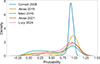 |
Fig. 8. Kernel density distribution of the classification probabilities assigned by our model to SySt candidates proposed in previous works. The Merc catalog includes literature-based candidates compiled between 2019 and November 2024. |
Comparison of our classification results with previously published catalogs of SySt candidates.
Our findings reveal strong agreement with recent catalogs that employed photometric and spectroscopic diagnostics aligned with our feature space, particularly those emphasizing Hα emission and consistent infrared properties. Meanwhile, observed differences with older or more heterogeneous samples highlight the importance of standardized parameter spaces and clearly defined selection criteria. Overall, these results support the effectiveness of trained and constrained MLs classifiers as robust tools for the large-scale identification of symbiotic systems, especially shell-burning types characterized by strong Hα emission and stable infrared signatures.
7. Summary and conclusions
We presented a new supervised classification method for identifying S-type SySt candidates based on an RF algorithm combined with SMOTE to address class imbalance. The model was trained with a set of astrometric, photometric, and spectroscopic features derived from Gaia DR3, 2MASS, and WISE data. Key input variables include color indices, parallax, and the EWHα line. These features define a restricted parameter space in which symbiotic systems are most likely to reside, enabling an efficient candidate selection.
The classifier demonstrated an excellent overall performance, especially in distinguishing non-SySt sources. While it remains more complex to classify the minority class (S-type SySt), the use of SMOTE helped us to mitigate the effects of class imbalance. To refine the candidate selection, we applied a classification probability threshold of 70%, selected to balance completeness and accuracy in the entire candidate sample.
By applying our model to a selected sample of over 2.5 million sources, we identified 990 high-probability candidates. The physical properties of 12 of these are consistent with known S-type SySts, including Hα emission and ultraviolet excess in the SkyMapper uvg bands. In addition, we identified a group of 133 candidates with similar photometric characteristics (i.e., blue optical colors and infrared excess). While their classification probabilities are high, the lack of complete astrophysical information (e.g., Teff or log g) prevented a more detailed evaluation in this work. Nevertheless, these sources represent strong candidates for future observations because they might host hot compact companions and constitute previously unknown interacting binary systems.
The model performance was verified independently with a validation set introduced by Lucy et al. (2025), which correctly recognized 11 of the 12 known S-type SySts (∼92.3%), demonstrating a robust predictive capability. Importantly, the model was trained and validated on a well-characterized dataset with broad coverage of the spectral energy distribution (SED), including spectroscopic features consistent with data availability in the Merc catalog. The application of the model to a larger dataset or to a dataset with coarse SED sampling might reduce its predictive reliability because the classifier cannot accurately recognize objects outside the parameter space on which it was trained. To further assess its robustness, we tested it on a sample of 155 photometric mimics reported by Merc et al. (2019) and found that 51 were incorrectly classified as symbiotic. This raised the contamination rate to ∼33%. These results confirm that the classifier performs reliably within its trained parameter space, but is sensitive to sources with incomplete or coarsely sampled SEDs.
We also applied our model to previously published candidate catalogs. The overall agreement is close to 50%, with greater consistency in samples incorporating Hα and infrared criteria. This agreement validates the robustness of our classifier. This bias might lead to an underrepresentation of accretion-only systems such as SU Lyn, whose emission lines are not as prominent as those of shell-burning systems. Furthermore, low-resolution spectra can underestimate the Hα intensity due to continuum contamination from the red giant. This highlights the need for caution in the emission-based selection.
The limited number of confirmed SySts, even when complemented by our new candidates, has significant implications for population synthesis models. While adding several hundred confirmed systems would establish meaningful lower bounds, our current census remains well below theoretical predictions, which reach (53 ± 6)×104 systems. This discrepancy might reflect observational biases, particularly against accretion-only systems with weak emission lines, or it might highlight an incomplete evolutionary modeling. It is essential to address this gap to advance our understanding of binary evolution and the Galactic symbiotic population.
Although infrared emission and Balmer emission lines are classic indicators of SySts, they are not an exclusive diagnostic. Other astrophysical sources can mimic these features, emphasizing the importance of a multiwavelength approach that integrates photometric and spectroscopic data to reduce contamination and improve the classification reliability for appropriate spectroscopic follow-up. In this context, we plan to retrain the model with new S-PLUS data, which offer a broader SED coverage and might enhance the classification performance. These observations are currently in progress, and the updated model will be presented in future work.
In general, we demonstrated that MLs are powerful tools for the automated discovery of rare astrophysical systems in large-scale public databases. When trained with carefully curated representative datasets, classifiers can effectively model complex relations between observables and generate high-confidence predictions. For SySts, the limited number of confirmed examples and the diversity of spectral manifestations pose significant challenges. Therefore, the results must be interpreted in an astrophysical context and validated through rigorous observational follow-up.
Acknowledgments
We thank the referee for their constructive comments and valuable suggestions, which helped to improve the clarity and quality of this manuscript. This work was supported by DIDULS/ULS through projects PTE23538510 and PTE23538516, as well as by the ANID FONDECYT project 1231637. M.J.A. acknowledge support from the ANID FONDECYT Iniciación 11251912. NEN and GJML are members of the CIC-CONICET (Argentina). This work presents results from the European Space Agency (ESA) space mission Gaia. Gaia data are being processed by the Gaia Data Processing and Analysis Consortium (DPAC). Funding for the DPAC is provided by national institutions, in particular the institutions participating in the Gaia MultiLateral Agreement (MLA). The Gaia mission website is https://www.cosmos.esa.int/gaia. The Gaia archive website is https://archives.esac.esa.int/gaia. This research has made use of the VizieR catalogue access tool, CDS, Strasbourg, France, as well as public data from the Two Micron All Sky Survey (2MASS) and the Wide-field Infrared Survey Explorer (WISE). 2MASS is a joint project of the University of Massachusetts and the Infrared Processing and Analysis Center/California Institute of Technology, funded by NASA and the NSF. WISE is a joint project of the University of California, Los Angeles, and the Jet Propulsion Laboratory/California Institute of Technology, funded by NASA. This work has also made use of data from the SkyMapper Southern Survey. The national facility capability for SkyMapper has been funded through ARC LIEF grant LE130100104 from the Australian Research Council, awarded to the University of Sydney, the Australian National University, Swinburne University of Technology, the University of Queensland, the University of Western Australia, the University of Melbourne, Curtin University of Technology, Monash University, and the Australian Astronomical Observatory. SkyMapper is owned and operated by the Australian National University’s Research School of Astronomy and Astrophysics. The survey data were processed and provided by the SkyMapper Team at ANU. The SkyMapper node of the All-Sky Virtual Observatory (ASVO) is hosted at the National Computational Infrastructure (NCI). Development and support of the SkyMapper node of the ASVO has been funded in part by Astronomy Australia Limited (AAL) and the Australian Government through the Commonwealth’s Education Investment Fund (EIF) and National Collaborative Research Infrastructure Strategy (NCRIS), particularly the National eResearch Collaboration Tools and Resources (NeCTAR) and the Australian National Data Service Projects (ANDS).
References
- Akras, S., Guzman-Ramirez, L., Leal-Ferreira, M. L., & Ramos-Larios, G. 2019a, ApJS, 240, 21 [NASA ADS] [CrossRef] [Google Scholar]
- Akras, S., Leal-Ferreira, M. L., Guzman-Ramirez, L., & Ramos-Larios, G. 2019b, MNRAS, 483, 5077 [NASA ADS] [CrossRef] [Google Scholar]
- Akras, S., Gonçalves, D. R., Alvarez-Candal, A., & Pereira, C. B. 2021, MNRAS, 502, 2513 [CrossRef] [Google Scholar]
- Akras, S., Leal-Ferreira, M. L., Guzman-Ramirez, L., & Ramos-Larios, G. 2022, VizieR On-line Data Catalog: J/MNRAS/483/5077 [Google Scholar]
- Allen, D. A. 1982, Astrophys. Space Sci. Libr., 95, 27 [Google Scholar]
- Anders, F., Khalatyan, A., Chiappini, C., et al. 2019, A&A, 628, A94 [NASA ADS] [CrossRef] [EDP Sciences] [Google Scholar]
- Angeloni, R., Contini, M., Ciroi, S., & Rafanelli, P. 2010, MNRAS, 402, 2075 [Google Scholar]
- Avdeeva, A. A., et al. 2023, Astron. Comput., 45, 100744 [Google Scholar]
- Ball, S. E., Bromley, B. C., & Kenyon, S. J. 2025, Open J. Astrophys., 8, 122 [Google Scholar]
- Belczyński, K., Mikołajewska, J., Munari, U., Ivison, R. J., & Friedjung, M. 2000, A&AS, 146, 407 [NASA ADS] [CrossRef] [EDP Sciences] [Google Scholar]
- Bessell, M., Bloxham, G., Schmidt, B., et al. 2011, PASP, 123, 789 [Google Scholar]
- Boller, T., Freyberg, M. J., Trümper, J., et al. 2016, A&A, 588, A103 [NASA ADS] [CrossRef] [EDP Sciences] [Google Scholar]
- Breiman, L. 2001, Mach. Learn., 45, 5 [Google Scholar]
- Buitinck, L., Louppe, G., Blondel, M., et al. 2013, in ECML PKDD Workshop: Languages for Data Mining and Machine Learning, 108 [Google Scholar]
- Chawla, N. V., Bowyer, K. W., Hall, L. O., & Kegelmeyer, W. P. 2002, J. Artif. Int. Res., 16, 321 [Google Scholar]
- Chen, C., Liaw, A., & Breiman, L. 2004, Technical Report (Berkeley: University of California) [Google Scholar]
- Chen, P. S., Liu, J. Y., & Shan, H. G. 2019, Ap&SS, 364, 132 [Google Scholar]
- Corradi, R. L. M., Mikolajewska, J., & Mahoney, T. J. 2003, ASP Conf. Ser., 303, 58381 [Google Scholar]
- Corradi, R. L. M., Rodríguez-Flores, E. R., Mampaso, A., et al. 2008, A&A, 480, 409 [NASA ADS] [CrossRef] [EDP Sciences] [Google Scholar]
- Creevey, O. L., Sordo, R., Pailler, F., et al. 2023, A&A, 674, A26 [NASA ADS] [CrossRef] [EDP Sciences] [Google Scholar]
- Cui, X.-Q., Zhao, Y.-H., Chu, Y.-Q., et al. 2012, Res. Astron. Astrophys., 12, 1197 [Google Scholar]
- Di Stefano, R. 2010, ApJ, 719, 474 [CrossRef] [Google Scholar]
- Dickey, J. M., Weston, J. H. S., Sokoloski, J. L., Vrtilek, S. D., & McCollough, M. 2021, ApJ, 911, 30 [Google Scholar]
- Drew, J. E., Greimel, R., Irwin, M. J., et al. 2005, MNRAS, 362, 753 [NASA ADS] [CrossRef] [Google Scholar]
- Evans, P. A., Page, K. L., Osborne, J. P., et al. 2020, ApJS, 247, 54 [Google Scholar]
- Gaia Collaboration (Prusti, T., et al.) 2016, A&A, 595, A1 [NASA ADS] [CrossRef] [EDP Sciences] [Google Scholar]
- Gaia Collaboration (Vallenari, A., et al.) 2023, A&A, 674, A1 [NASA ADS] [CrossRef] [EDP Sciences] [Google Scholar]
- Gałan, C., Mikołajewska, J., Hinkle, K. H., & Joyce, R. R. 2017, MNRAS, 466, 2194 [CrossRef] [Google Scholar]
- Gałan, C., Mikołajewska, J., Hinkle, K. H., & Joyce, R. R. 2023, MNRAS, 526, 918 [CrossRef] [Google Scholar]
- Green, G., Edenhofer, G., Krughoff, S., et al. 2024, https://doi.org/10.5281/zenodo.10517733 [Google Scholar]
- Gromadzki, M., Mikołajewska, J., Borawska, M., & Lednicka, A. 2007, Baltic Astron., 16, 37 [NASA ADS] [Google Scholar]
- Hosenie, Z., Scaringi, S., Balona, L., & Snaid, S. 2020, MNRAS, 493, 6050 [NASA ADS] [CrossRef] [Google Scholar]
- Ivison, R. J., Seaquist, E. R., Schwarz, H. E., Hughes, D. H., & Bode, M. F. 1995, MNRAS, 273, 517 [Google Scholar]
- Jia, Y., Guo, S., Zhu, C., et al. 2023, Res. Astron. Astrophys., 23, 105012 [CrossRef] [Google Scholar]
- Kenny, H. T., & Taylor, A. R. 2005, ApJ, 619, 527 [Google Scholar]
- Kenyon, S. J. 1986, The symbiotic stars [Google Scholar]
- Kenyon, S. J., Livio, M., Mikolajewska, J., & Tout, C. A. 1993, ApJ, 407, L81 [CrossRef] [Google Scholar]
- Kilpio, E., & Bisikalo, D. 2009, Ap&SS, 320, 141 [Google Scholar]
- Kolmogorov, A. N. 1933, Giornale dell’Istituto Italiano degli Attuari, 4, 83 [Google Scholar]
- Laversveiler, M., Gonçalves, D. R., Rocha-Pinto, H. J., & Merc, J. 2025, A&A, 698, A155 [NASA ADS] [CrossRef] [EDP Sciences] [Google Scholar]
- Lemaître, G., Nogueira, F., & Aridas, C. K. 2017, J. Mach. Learn. Res., 18, 1 [Google Scholar]
- Li, J., Mikołajewska, J., Chen, X.-F., et al. 2015, Res. Astron. Astrophys., 15, 1332 [Google Scholar]
- Lindegren, L., Bastian, U., Biermann, M., et al. 2020, A&A, 649, A4 [Google Scholar]
- Lü, G., Yungelson, L., & Han, Z. 2006, MNRAS, 372, 1389 [CrossRef] [Google Scholar]
- Lucy, A. B., Sokoloski, J. L., Luna, G. J. M., et al. 2025, MNRAS, 543, 2292 [Google Scholar]
- Luna, G. J. M., Sokoloski, J. L., Mukai, K., & Nelson, T. 2013, A&A, 559, A6 [NASA ADS] [CrossRef] [EDP Sciences] [Google Scholar]
- Lundberg, S. M., & Lee, S.-I. 2017, in Proceedings of the 31st International Conference on Neural Information Processing Systems, NIPS’17 (Red Hook, NY, USA: Curran Associates Inc.), 4768 [Google Scholar]
- Magrini, L., Corradi, R. L. M., & Munari, U. 2003, ASP Conf. Ser., 303, 539 [NASA ADS] [Google Scholar]
- Maravelias, G., Bonanos, A. Z., Raddi, R., et al. 2022, A&A, 666, A122 [NASA ADS] [CrossRef] [EDP Sciences] [Google Scholar]
- Medina Tanco, G. A., & Steiner, J. E. 1995, AJ, 109, 1770 [Google Scholar]
- Merc, J. 2022, Ph.D. Thesis, Charles University in Prague/P. J. Šafárik University in Košice, Czech Republic/Slovakia [Google Scholar]
- Merc, J. 2025, Galaxies, 13, 49 [Google Scholar]
- Merc, J., Gàlis, R., & Wolf, M. 2019, Eruptive Stars Inf. Lett., 41, 78 [Google Scholar]
- Merc, J., Gális, R., Vrašt’ák, M., et al. 2021, Open Eur. J. Variable Stars, 220, 11 [Google Scholar]
- Mikołajewska, J. 2012, Baltic Astron., 21, 5 [Google Scholar]
- Muerset, U., Nussbaumer, H., Schmid, H. M., & Vogel, M. 1991, A&A, 248, 458 [Google Scholar]
- Muerset, U., Wolff, B., & Jordan, S. 1997, A&A, 319, 201 [Google Scholar]
- Mukai, K., Luna, G. J. M., Cusumano, G., et al. 2016, MNRAS, 461, L1 [NASA ADS] [CrossRef] [Google Scholar]
- Mukai, K., Luna, G., Nelson, T., et al. 2017, AAS/High Energy Astrophys. Div., 16, 108.06 [Google Scholar]
- Munari, U. 2019, ArXiv e-prints [arXiv:1909.01389] [Google Scholar]
- Munari, U., & Dallaporta, S. 2021, ATel., 15066, 1 [Google Scholar]
- Munari, U., & Renzini, A. 1992, ApJ, 397, L87 [NASA ADS] [CrossRef] [Google Scholar]
- Mürset, U., & Schmid, H. M. 1999, A&AS, 137, 473 [NASA ADS] [CrossRef] [EDP Sciences] [Google Scholar]
- Onken, C. A., Wolf, C., Bessell, M. S., et al. 2019, PASA, 36, e033 [Google Scholar]
- Powers, D. 2011, J. Mach. Learn. Technol., 2, 37 [NASA ADS] [Google Scholar]
- Recio-Blanco, A., de Laverny, P., Palicio, P. A., et al. 2023, A&A, 674, A29 [NASA ADS] [CrossRef] [EDP Sciences] [Google Scholar]
- Rodríguez-Flores, E. R., Corradi, R. L. M., Mampaso, A., et al. 2014, A&A, 567, A49 [CrossRef] [EDP Sciences] [Google Scholar]
- Schlegel, D. J., Finkbeiner, D. P., & Davis, M. 1998, ApJ, 500, 525 [Google Scholar]
- Shridharan, B., Mathew, B., Bhattacharyya, S., et al. 2022, A&A, 668, A156 [NASA ADS] [CrossRef] [EDP Sciences] [Google Scholar]
- Skrutskie, M. F., Cutri, R. M., Stiening, R., et al. 2006, AJ, 131, 1163 [NASA ADS] [CrossRef] [Google Scholar]
- Smirnov, N. V. 1948, Ann. Math. Stat., 19, 279 [CrossRef] [Google Scholar]
- Sokoloski, J. L. 2003, ASP Conf. Ser., 303, 202 [Google Scholar]
- Stoyanov, K. A., Martí, J., Zamanov, R., et al. 2018, Bulgarian Astron. J., 28, 42 [Google Scholar]
- Taylor, M. B. 2005, ASP Conf. Ser., 347, 29 [Google Scholar]
- Wang, B., Liu, Z., Han, Y., et al. 2010, Sci. China Phys. Mech. Astron., 53, 586 [Google Scholar]
- Webster, B. L., & Allen, D. A. 1975, MNRAS, 171, 171 [NASA ADS] [CrossRef] [Google Scholar]
- Wenger, M., Ochsenbein, F., Egret, D., et al. 2000, A&AS, 143, 9 [NASA ADS] [CrossRef] [EDP Sciences] [Google Scholar]
- Wright, E. L., Eisenhardt, P. R. M., Mainzer, A. K., et al. 2010, AJ, 140, 1868 [Google Scholar]
- Xu, X.-J., Shao, Y., & Li, X.-D. 2024, ApJ, 962, 126 [NASA ADS] [CrossRef] [Google Scholar]
- Zamanov, R., Latev, G., Boeva, S., et al. 2015, MNRAS, 450, 3958 [NASA ADS] [CrossRef] [Google Scholar]
https://sirrah.troja.mff.cuni.cz/~merc/nodsv/, accessed in April 2024.
Appendix A: ADQL query used for the initial sample extraction
The following ADQL query was used to extract the initial candidate sample from Gaia DR3, cross-matched with 2MASS and including astrophysical parameters. The selection criteria were defined to match the parameter space covered by the confirmed symbiotic stars used for training, ensuring consistency between the training and application domains.
SELECT
    gaia.source_id, gaia.*, ap.*, tmass.*
FROM gaiadr3.gaia_source AS gaia
JOIN gaiadr3.tmass_psc_xsc_best_neighbour AS xmatch USING (source_id)
JOIN gaiadr3.tmass_psc_xsc_join AS xjoin USING (clean_tmass_psc_xsc_oid)
JOIN gaiadr1.tmass_original_valid AS tmass
    ON xjoin.original_psc_source_id = tmass.designation
JOIN gaiadr3.astrophysical_parameters AS ap
    USING (source_id)
WHERE
    gaia.phot_g_mean_mag - gaia.phot_rp_mean_mag BETWEEN 0.29 AND 2.34
    AND gaia.phot_g_mean_mag - gaia.phot_bp_mean_mag BETWEEN -4.19 AND 0.10
    AND gaia.phot_bp_mean_mag - gaia.phot_rp_mean_mag BETWEEN 0.22 AND 5.95
    AND gaia.phot_g_mean_mag < 16
    AND gaia.parallax IS NOT NULL
    AND gaia.parallax_over_error > 10.00
    AND ap.ew_espels_halpha IS NOT NULL
    AND ap.ew_espels_halpha BETWEEN -18.49 AND 0.69
    AND tmass.j_m - tmass.h_m BETWEEN 0.22 AND 2.99
    AND tmass.j_m - tmass.ks_m BETWEEN 0.46 AND 5.33
    AND tmass.h_m - tmass.ks_m BETWEEN 0.11 AND 2.34
Appendix B: Kolmogorov–Smirnov tests for negative-class subsampling
Two-sample KS test comparing the selected negative subset (1 600 sources) with the full negative population (∼150 000).
Appendix C: Local SHAP explanation for a misclassified validation source
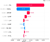 |
Fig. C.1. SHAP waterfall plot showing the local explanation of the classifier prediction for the validation source V V1918 Sgr*. Positive contributions increase the predicted probability of the symbiotic class relative to the baseline. |
All Tables
Performance scores per class for the RF classifier applied to the test sample with their respective standard deviation.
Comparison of our classification results with previously published catalogs of SySt candidates.
Two-sample KS test comparing the selected negative subset (1 600 sources) with the full negative population (∼150 000).
All Figures
|
Fig. 1. Average number of valid measurements per photometric group in the sample. Each bar represents the mean number of available (not missing) values for the bands belonging to a given instrument or spectral range. |
| In the text | |
|
Fig. 2. Color–color selection process. Left: 2D histogram of approximately 17 988 392 sources obtained from four ADQL queries to the Gaia services and a WISE cross-match. The first selection cut was applied in the Gaia color–color diagram using a linear regression in logarithmic scale, resulting in the removal of 143 434 sources. Confirmed SySts are marked as orange stars. Right: 2D histogram of over 4 million sources selected from the 2MASS color–color diagram. The color bar indicates the number of sources per bin in logarithmic scale for both panels. |
| In the text | |
|
Fig. 3. Distribution of the training set characteristics for the positive class (S-type SySts) and the negative class (“others”). |
| In the text | |
|
Fig. 4. Confusion matrix for the testing set using SMOTE + RF, incorporating photometric colors, parallax, and EWHα. The x-axis represents the predicted class (predicted label), and the y-axis denotes the actual class (true label). Each cell shows the percentage relative to its respective class on the first line, followed by the corresponding number of stars on the second line. |
| In the text | |
|
Fig. 5. Comparison between the mean impurity decay of random forest (MDI, orange bars) and the importance of permutation features calculated using the F1 score (black dots). |
| In the text | |
|
Fig. 6. Galactic distribution of 990 SySt candidates (purple points) according to our model and confirmed S-type of SySts (orange stars). |
| In the text | |
|
Fig. 7. Color-color plot of the SkyMapper u − v vs. u − g photometry for our candidates (gray dots), known SySts (orange dots), and the 12 most likely candidates (purple dots). |
| In the text | |
|
Fig. 8. Kernel density distribution of the classification probabilities assigned by our model to SySt candidates proposed in previous works. The Merc catalog includes literature-based candidates compiled between 2019 and November 2024. |
| In the text | |
|
Fig. C.1. SHAP waterfall plot showing the local explanation of the classifier prediction for the validation source V V1918 Sgr*. Positive contributions increase the predicted probability of the symbiotic class relative to the baseline. |
| In the text | |
Current usage metrics show cumulative count of Article Views (full-text article views including HTML views, PDF and ePub downloads, according to the available data) and Abstracts Views on Vision4Press platform.
Data correspond to usage on the plateform after 2015. The current usage metrics is available 48-96 hours after online publication and is updated daily on week days.
Initial download of the metrics may take a while.