© The Authors 2026

1. Introduction

The most widely accepted cosmological model that remains consistent with observational data is the λ cold dark matter (ΛCDM) model of a spatially flat universe. This model proposes that the cosmological constant Λ, assumed to represent dark energy, drives the accelerated expansion of the Universe (Carroll et al. 1992; Riess et al. 1998; Perlmutter et al. 1999; Carroll 2001; Peebles & Ratra 2003; Frieman et al. 2008; Weinberg et al. 2013; Planck Collaboration VI 2020), while cold dark matter (CDM) behaves as a nonrelativistic, pressureless perfect fluid. However, the ΛCDM model faces several significant issues (Weinberg 1989). For example, it cannot explain the physical nature of CDM or Λ (Weinberg 1989; Padmanabhan 2003) and, additionally, it fails to solve the fine-tuning problem; specifically, the question of why Λ is so small compared to the vacuum energy predicted by quantum field theory (Zel’dovich 1968; Weinberg 1989; Padmanabhan 2003; Sanchez 2021). It also does not address the coincidence problem, which asks why Λ does not become dynamically relevant until the late Universe (Zlatev et al. 1999). Collectively, these unresolved issues are known as the cosmological constant problem (Weinberg 1989).

With the increasing precision of cosmological observations, several tensions related to key parameters have emerged; most notably the so-called “Hubble tension”, which arises from the inconsistency between the values of the Hubble constant H₀ derived from early Universe measurements and local (late-time) observations. The Planck Collaboration, using observations of the cosmic microwave background (CMB) within the ΛCDM framework, reported H₀ = (67.36 ± 0.54) km s⁻¹ Mpc⁻¹ at a 68% confidence level (CL). In contrast, the SH0ES Collaboration (Supernovae H₀ for the equation of state, EoS) found a significantly higher value of H₀ = (73.04 ± 1.04) km s⁻¹ Mpc⁻¹ at 68% CL, using the three-rung distance ladder method with Cepheids (Riess et al. 2022). These results reveal a tension of approximately 5σ, which is unlikely to be due to systematic errors and, thus, strongly suggests there is a need for new physics beyond the ΛCDM model. A comprehensive review of proposals aimed at addressing the Hubble tension can be found in Di Valentino et al. (2021), Moresco et al. (2022), Verde et al. (2024), Perivolaropoulos (2024), Mörtsell et al. (2022).

For these reasons, in recent decades, a wide variety of alternatives to the standard cosmological model have been proposed. In most of these proposals, cosmic components are modeled as perfect fluids. Among them, scalar field models with a dynamical EoS have attracted significant attention. Quintessence models offer a dynamical alternative to Λ (e.g., Caldwell et al. 1998; Di Valentino et al. 2019), while phantom (Caldwell 2002) and k-essence models (Chiba 2002) extend the framework to EoS parameters ω < −1 or to noncanonical kinetic terms. Additionally, various reviews of dark energy and modified gravity models can be found in Copeland et al. (2006), Bamba et al. (2012).

Among the alternative approaches, a less conventional one modifies the dark sector by introducing dissipative terms into the energy-momentum tensor to generate accelerated expansion (Avelino & Nucamendi 2010; Cruz et al. 2017, 2023), while also attempting to alleviate current cosmological tensions (Anand et al. 2017; Yang et al. 2019; Ashoorioon & Davari 2023). These contributions include heat flux (Bravo Medina et al. 2019), bulk viscous pressure, and shear viscosity. The most extensively studied cosmological models with viscous fluids incorporate bulk viscosity, as they remain compatible with the cosmological principle. In contrast, shear viscosity introduces tensor terms that explicitly violate isotropy.

Among the theories that describe viscous fluids, the first to address bulk viscosity was Eckart’s theory (Eckart 1940). Although this formalism suffers from well-known causality issues, its mathematical simplicity has made it widely studied, providing a fundamental first-order approximation for dissipative fluids. Israel and Stewart later proposed a causal second-order theory (Israel 1976; Israel & Stewart 1979), introducing relaxation time as a new parameter.

A bulk viscous fluid is characterized by two key thermodynamic quantities: the energy density, ρ, and the effective pressure, P_eff = p + Π, where p is the equilibrium pressure and Π denotes the bulk viscous pressure. Within Eckart’s first-order formalism, the viscous pressure takes the form Π = −ζϑ, where ζ is the bulk viscosity coefficient and $\vartheta \equiv u_{;\mu }^{\mu }=3H$ is the expansion scalar, with H ≡ ȧ/a being the Hubble parameter. The Israel-Stewart theory extends this description by introducing a propagation equation for Π that resolves the causality limitations of Eckart’s approach.

Both the Eckart and Israel-Stewart theories can account for the accelerated expansion of the Universe without a cosmological constant, provided that Π < 0 (and, consequently, ζ > 0) to satisfy the second law of thermodynamics (Weinberg 1972). However, analyses of dissipative inflation (Maartens 1995) reveal a fundamental limitation: models relying exclusively on bulk viscosity to drive acceleration violate the near-equilibrium condition |Π/p|≪1, which is required to maintain the system close to local thermal equilibrium. This violation implies that purely viscous mechanisms cannot realistically drive cosmic acceleration without additional components.

This motivates our inclusion of Λ, supported by observational evidence for its cosmological role (Riess et al. 1998; Perlmutter et al. 1999; Bennett et al. 2013). Recent studies (Cruz et al. 2018; Herrera-Zamorano et al. 2020; Cruz et al. 2022a,b) show that a positive Λ can preserve near-equilibrium conditions in certain regimes, although this requires moving beyond unified viscous dark matter models as complete descriptions of late-time cosmology.

Given that cosmic matter exhibits dissipation (Anand et al. 2018), here we analyze viscous cold dark matter (vCDM) models within Eckart’s theory in the presence of Λ, following the background dynamics framework presented in (Velten & Schwarz 2012; Velten et al. 2014). We denote these models as ΛvCDM. We explore two particular scenarios: (i) constant bulk viscosity (ζ = ζ₀, where ζ₀ is the present-day value) and (ii) variable bulk viscosity (ζ = ζ(Ω_vc)), where Ω_vc denotes the vCDM energy density parameter. We study both scenarios in flat and curved FLRW universes, where Π modifies the effective energy-momentum tensor. Therefore, this framework extends the ΛCDM model by introducing dissipative effects in the dark matter component.

This paper is organized as follows. In Section 2, we explain the theoretical framework underpinning bulk viscous models. We describe the methodology and datasets employed to constrain the cosmological parameters in Section 3. In Section 4, we present and discuss the resulting constraints on various cosmological parameters, including their concordance with the benchmark ΛCDM model, evaluated using information criteria and Bayesian inference. Finally, in Section 5, we summarize our conclusions.

2. Background for bulk viscous models

A homogeneous and isotropic universe is described by the FLRW metric, given by

$$\begin{array}{c}\hfill \mathrm{d}{s}^2=-c^2\mathrm{d}{t}^2+a^2(t)(\frac{\mathrm{d}{r}^2}{1-K{r}^2}+r^2\mathrm{d}{\theta }^2+r^2{sin}^2\theta \mathrm{d}{\varphi }^2),\end{array}$$(1)

where (r, θ, ϕ) are the comoving coordinates, a(t) is the scale factor at cosmic time, t, and K denotes the spatial curvature parameter. The values of K = −1, 0, +1 correspond to an open, flat, and closed universe, respectively.

We assume a universe containing a component that experiences dissipative processes exclusively through bulk viscosity. This introduces a nonadiabatic contribution (ΔT^μν) to the perfect fluid energy-momentum tensor (Weinberg 1972). Therefore, the total energy-momentum tensor for a bulk viscous fluid takes the form of

$$\begin{array}{c}\hfill \begin{array}{cc}\hfill T^{\mu \nu }& \equiv {\mathcal{T}}^{\mu \nu }+\mathrm{\Delta }{T}^{\mu \nu }\hfill \\ \hfill & =(\rho +P_{\mathrm{eff}})u^{\mu }{u}^{\nu }+P_{\mathrm{eff}}{g}^{\mu \nu },\hfill \end{array}\end{array}$$(2)

where 𝒯^μν is the energy-momentum tensor that describes a perfect fluid and the four-velocity satisfies the normalization condition u^μu_μ = −1. In the Eckart framework, bulk viscosity modifies the equilibrium pressure p to an effective pressure,

$$\begin{array}{c}\hfill P_{\mathrm{eff}}=p-3H\zeta ,\end{array}$$(3)

where p ≡ ωρ follows a barotropic EoS. The dimensionless parameter ω can be constant (e.g., ω = 0 for CDM or ω = −1 for Λ) or time-dependent, as in dynamical dark energy models (see Caldwell et al. 1998; Chiba 2002).

When vCDM is the only viscous component in a universe with noninteracting cosmic fluids, its energy-momentum conservation (derived from ∇_μT^μν = 0) yields

$$\begin{array}{c}\hfill {\dot{\rho }}_{\mathrm{vc}}+3H{\rho }_{\mathrm{vc}}=9\zeta H^2,\end{array}$$(4)

where ρ_vc and p_vc = 0 are the energy density and pressure of the vCDM component (abbreviated as ‘vc’ in equations), respectively. The corresponding Friedmann equations, including spatial curvature and the cosmological constant, are

$$\begin{array}{cc}& H^2=\frac{8\pi G}{3c^2}({\rho }_{\mathrm{r}}+{\rho }_{\mathrm{b}}+{\rho }_{\mathrm{vc}})-\frac{K{c}^2}{a^2}+\frac{\mathrm{\Lambda }{c}^2}{3},\hfill \end{array}$$(5)

$$\begin{array}{cc}& 2\dot{H}+3H^2=-\frac{8\pi G}{c^2}(p_{\mathrm{r}}+p_{\mathrm{b}}+p_{\mathrm{vc}}-3\zeta H)-\frac{K{c}^2}{a^2}+\mathrm{\Lambda }{c}^2,\hfill \end{array}$$(6)

where G is Newton’s gravitational constant. The subscripts r and b denote radiation and baryonic matter, respectively. Combining the scale factor-redshift relation a(t) = (1 + z)⁻¹ with Eq. (5) yields the normalized Hubble parameter E(z)≡H(z)/H₀ for our ΛvCDM model, including spatial curvature, expressed as

$$\begin{array}{c}\hfill \begin{array}{cc}\hfill E(z)=[{\mathrm{\Omega }}_{\mathrm{r}0}{(1+z)}^4+{\mathrm{\Omega }}_{\mathrm{vc}}(z)& +{\mathrm{\Omega }}_{\mathrm{b}0}{(1+z)}^3\hfill \\ \hfill & +{\mathrm{\Omega }}_{\mathrm{K}0}{(1+z)}^2+{\mathrm{\Omega }}_{\mathrm{\Lambda }}{]}^{1/2},\hfill \end{array}\end{array}$$(7)

where H₀ = 100 h km s⁻¹ Mpc⁻¹ is the Hubble constant, while h is the dimensionless Hubble parameter. The energy density parameter of vCDM is defined as

$$\begin{array}{c}\hfill {\mathrm{\Omega }}_{\mathrm{vc}}(z)\equiv \frac{{\rho }_{\mathrm{vc}}}{{\rho }_{\mathrm{crit},0}}=\frac{8\pi G{\rho }_{\mathrm{vc}}(z)}{3H_0^2{c}^2},\end{array}$$(8)

and its present-day is Ω_vc(z = 0) = Ω_vc0. The remaining set, Ω_r0, Ω_b0, Ω_K0, and Ω_Λ ≡ Ω_de(z = 0) are defined as

$$\begin{array}{c}\hfill \begin{array}{cc}& {\mathrm{\Omega }}_{\mathrm{r}0}=\frac{8\pi G{\rho }_{\mathrm{r}0}}{3H_0^2{c}^2};{\mathrm{\Omega }}_{\mathrm{b}0}=\frac{8\pi G{\rho }_{\mathrm{b}0}}{3H_0^2{c}^2};\hfill \\ \hfill & {\mathrm{\Omega }}_{\mathrm{K}0}=\frac{8\pi G{\rho }_{\mathrm{K}0}}{3H_0^2{c}^2};{\mathrm{\Omega }}_{\mathrm{\Lambda }}=\frac{8\pi G{\rho }_{\mathrm{\Lambda }}}{3H_0^2{c}^2}·\hfill \end{array}\end{array}$$(9)

The sum of these present-day density parameters satisfies the constraint,

$$\begin{array}{c}\hfill {\mathrm{\Omega }}_{\mathrm{r}0}+{\mathrm{\Omega }}_{\mathrm{b}0}+{\mathrm{\Omega }}_{\mathrm{vc}0}+{\mathrm{\Omega }}_{\mathrm{K}0}+{\mathrm{\Omega }}_{\mathrm{\Lambda }}=1.\end{array}$$(10)

For radiation, we use Ω_r0 ≈ (1+0.2271 N_eff)Ω_γ0, where Ω_γ0 = 2.469 ⋅ 10⁻⁵ h⁻² (Komatsu et al. 2011) is the present-day photon density parameter and N_eff = 3.046 is the effective number of neutrino species according to the standard ΛCDM model (Mangano et al. 2002, 2005).

We can rewrite Eq. (4) in terms of dimensionless quantities, as in Velten & Schwarz (2012), Velten et al. (2014), and solve it numerically by imposing the initial condition, Ω_vc(z = 0) = Ω_vc0. Introducing the notation ′ ≡ d/dz, we obtain

$$\begin{array}{c}\hfill \begin{array}{cc}\hfill (1+z){\mathrm{\Omega }}_{\mathrm{vc}}\prime & -3{\mathrm{\Omega }}_{\mathrm{vc}}(z)+{\zeta }^{\ast }[{\mathrm{\Omega }}_{\mathrm{r}0}{(1+z)}^4+{\mathrm{\Omega }}_{\mathrm{vc}}(z)\hfill \\ \hfill & {+{\mathrm{\Omega }}_{\mathrm{b}0}{(1+z)}^3+{\mathrm{\Omega }}_{\mathrm{K}0}{(1+z)}^2+{\mathrm{\Omega }}_{\mathrm{\Lambda }}]}^{1/2}=0,\hfill \end{array}\end{array}$$(11)

where we have defined the dimensionless viscosity parameter,

$$\begin{array}{c}\hfill {\zeta }^{\ast }=\frac{24\pi G}{c^2}\frac{\zeta }{H_0}·\end{array}$$(12)

We also derive the corresponding evolution equation for the Hubble parameter,

$$\begin{array}{c}\hfill \begin{array}{cc}& 2(1+z)HH\prime -3H^2+{\zeta }^{\ast }H{H}_0\hfill \\ \hfill & -H_0^2[{\mathrm{\Omega }}_{\mathrm{r}0}{(1+z)}^4-{\mathrm{\Omega }}_{\mathrm{K}0}{(1+z)}^2-3{\mathrm{\Omega }}_{\mathrm{\Lambda }}]=0.\hfill \end{array}\end{array}$$(13)

Each model is characterized by the bulk viscosity parameter ζ, as defined in Eq. (12), and it is reduced to the standard ΛCDM model when ζ = 0. We then adopt a power law dependence of viscosity on vCDM density,

$$\begin{array}{c}\hfill \zeta ={\zeta }_0{\left(\frac{{\mathrm{\Omega }}_{\mathrm{vc}}}{{\mathrm{\Omega }}_{\mathrm{vc}0}}\right)}^m,\end{array}$$(14)

where m is the viscous exponent and ζ₀ denotes the present-day bulk viscosity coefficient. Substituting the viscosity ansatz Eq. (14) into Eq. (12), we obtain (Velten & Schwarz 2012):

$$\begin{array}{c}\hfill {\zeta }^{\ast }=\stackrel{\sim }{{\zeta }_0}{\left(\frac{{\mathrm{\Omega }}_{\mathrm{vc}}}{{\mathrm{\Omega }}_{\mathrm{vc}0}}\right)}^m,\mathrm{with}{\stackrel{\sim }{\zeta }}_0=\frac{24\pi G}{c^2}\frac{{\zeta }_0}{H_0}·\end{array}$$(15)

Here, ${\stackrel{\sim }{\zeta }}_0$ is the dimensionless bulk viscosity parameter. In SI units, ζ has dimensions of Pascal-seconds (Pa s), while H₀ is expressed in inverse seconds (s⁻¹).

In this work, we study bulk viscous models with Λ, considering both spatially flat and curved geometries, labeled as ΛvCDM and ΛvCDM + Ω_K, respectively. Based on Eq. (15), we analyze two cases: (i) a constant bulk viscosity with m = 0, representing the simplest scenario; and (ii) a variable bulk viscosity with m treated as a free parameter. This defines four distinct bulk viscous models: ΛvCDM (m = 0), ΛvCDM + Ω_K (m = 0), ΛvCDM (m free), and ΛvCDM + Ω_K (m free). Additionally, we analyze the ${\stackrel{\sim }{\zeta }}_0=0$ case (the benchmark ΛCDM model) in Appendix B. The free parameters for each model are listed in Table 1.

3. Methodology and dataset for observational constraints

In this section, we focus on constraining the bulk viscous models using publicly available observational data. To achieve this, we utilized recent datasets, including Hubble parameter measurements from cosmic chronometers (CC) and baryon acoustic oscillations (BAOs), along with Type Ia supernovae (SNe Ia) data. The subsections below describe each dataset and the applied methodology.

3.1. Bayesian statistical procedure

Bayesian inference is a robust statistical technique for parameter estimation and model comparison, widely employed in cosmology. Based on Bayes’ theorem, the posterior probability of a model ℳ with free parameters, Θ, given a dataset, 𝒟, is expressed as

$$\begin{array}{c}\hfill \mathcal{P}(\mathrm{\Theta }|\mathcal{D},\mathcal{M})=\frac{\mathcal{L}(\mathcal{D}|\mathrm{\Theta },\mathcal{M})\pi (\mathrm{\Theta }|\mathcal{M})}{\mathcal{E}(\mathcal{D}|\mathcal{M})},\end{array}$$(16)

where 𝒫(Θ | 𝒟, ℳ) is the posterior distribution, ℒ(𝒟|Θ, ℳ) is the likelihood, π(Θ|ℳ) is the prior, and ℰ(𝒟|ℳ) is the evidence (also known as Bayesian evidence, marginal likelihood, or model likelihood).

A Gaussian likelihood is related to χ² statistic (usually called chi-square) via the relation ℒ ∝ e^−χ2/2, where χ² quantifies the discrepancy between observed data and model predictions. The best-fit parameters, corresponding to the maximum likelihood estimate, can be obtained by minimizing the χ² function.

3.1.1. Bayesian evidence

The evidence is a normalization constant in parameter estimation, which is crucial for model comparison. It is obtained by integrating the likelihood multiplied by the prior over the full parameter space,

$$\begin{array}{c}\hfill \mathcal{E}(\mathcal{D}|\mathcal{M})={\displaystyle \int \mathrm{d}}\mathrm{\Theta }\mathcal{L}(\mathcal{D}|\mathrm{\Theta },\mathcal{M})\pi (\mathrm{\Theta }|\mathcal{M}).\end{array}$$(17)

For two competing models, ℳ₀ and ℳ_i, the relative posterior probabilities (or posterior odds) determine which model is favored by the data, 𝒟,

$$\begin{array}{c}\hfill \frac{\mathcal{P}({\mathcal{M}}_0|\mathcal{D})}{\mathcal{P}({\mathcal{M}}_i|\mathcal{D})}=\frac{\mathcal{E}(\mathcal{D}|{\mathcal{M}}_0)\pi ({\mathcal{M}}_0)}{\mathcal{E}(\mathcal{D}|{\mathcal{M}}_i)\pi ({\mathcal{M}}_i)}={\mathcal{B}}_{0i}\frac{\pi ({\mathcal{M}}_0)}{\pi ({\mathcal{M}}_i)},\end{array}$$(18)

where ℬ_0i ≡ ℰ₀/ℰ_i is the Bayes factor, which quantifies the relative evidence for the models. Values of ℬ_0i > 1 indicate an increase in the support for ℳ₀ over ℳ_i, while ℬ_0i < 1 favors ℳ_i.

We adopted the Jeffreys scale, as suggested by Trotta (2008), Heavens et al. (2017b), to interpret the strength of evidence, as summarized in Table 2. When lnℬ_0i > 1, this suggests a preference for ℳ₀; conversely, when lnℬ_0i < −1, the data support the alternative model, ℳ_i.

3.1.2. Information criteria for the model comparison

A natural question is how efficient these models are compared to the standard ΛCDM model. To address this, we employed the Akaike information criterion (AIC; Akaike 1974), Bayesian information criterion (BIC; Schwarz 1978), and the deviance information criterion (DIC; Spiegelhalter et al. 2002). The AIC and BIC quantify the trade-off between goodness of fit and model complexity by penalizing the inclusion of additional free parameters. They are defined, respectively, as

$$\begin{array}{cc}\hfill \mathrm{AIC}& ={\chi }_{\min }^2+2k,\hfill \end{array}$$(19)

$$\begin{array}{cc}\hfill \mathrm{BIC}& ={\chi }_{\min }^2+klnN,\hfill \end{array}$$(20)

where χ_min² is the minimum chi-square value obtained from the best-fit parameters, k represents the number of free parameters, and N is the total number of data points used in the fit. The BIC penalizes additional parameters more strongly than the AIC, thus favoring simpler models. In both cases, the preferred model is the one that minimizes the corresponding information criterion.

The DIC combines concepts from Bayesian statistics and information theory. Unlike the AIC and BIC, the DIC determines the complexity penalty from the posterior distribution. It is defined as

$$\begin{array}{c}\hfill \mathrm{DIC}\equiv D(\overline{\mathrm{\Theta }})+2{\mathcal{C}}_B=\overline{D(\mathrm{\Theta })}+{\mathcal{C}}_B,\end{array}$$(21)

where ${\mathcal{C}}_B=\overline{D(\mathrm{\Theta })}-D(\overline{\mathrm{\Theta }})$ is the Bayesian complexity, quantifying the effective number of parameters. The overlines denote posterior mean values, and D(Θ) is the Bayesian deviance. For Gaussian likelihoods, the deviance is reduced to D(Θ) = χ²(Θ).

We can evaluate the relative strength of evidence for each candidate model i by calculating the differences in information criteria (ΔIC) relative to the benchmark ΛCDM model, defined as

$$\begin{array}{c}\hfill \mathrm{\Delta }\mathrm{IC}={\mathrm{IC}}_{\mathrm{\Lambda }\mathrm{CDM}}-{\mathrm{IC}}_i.\end{array}$$(22)

With this definition, positive values of ΔIC indicate a preference for model i over ΛCDM. We interpret the strength of evidence according to the standard scale summarized in Table 3.

3.2. Observational datasets

3.2.1. Cosmic chronometers

The most direct way to constrain the cosmological parameters is using H(z) data. We compiled a sample of 33 data points from various sources (shown in Table A.1), measured in the redshift range 0.07 ≤ z ≤ 1.965, where the total error per redshift is given by σ_tot = [σ_stat² + σ_syst²]^1/2. These H(z) data points were obtained using the CC method, which relies on comparing the differential age evolution of galaxies at different redshifts, as proposed by Jimenez & Loeb (2002). The method estimates the Hubble rate based on the relationship,

$$\begin{array}{c}\hfill H(z)=-\frac{1}{1+z}\frac{\mathrm{d}z}{\mathrm{d}t}·\end{array}$$(23)

This approach is independent of cosmological assumptions, making it a valuable tool for testing different models by directly measuring the expansion rate of the Universe.

By constructing the chi-square function, we effectively constrain the free parameters of the bulk viscous models. To perform the MCMC analysis, the χ² function for the CC method is given by

$$\begin{array}{c}\hfill {\chi }_{\mathrm{CC}}^2(\mathrm{\Theta })={\displaystyle \sum _{i=1}^{33}}{\left(\frac{H^{\mathrm{th}}(z_i,\mathrm{\Theta })-H_{\mathrm{CC}}^{\mathrm{obs}}(z_i)}{{\sigma }_{i,\mathrm{CC}}}\right)}^2,\end{array}$$(24)

where H_th(z_i, Θ) represents the theoretical value of the Hubble parameter at redshift, z_i, with the free model parameters, Θ, shown in Table 1, $H_{\mathrm{CC}}^{\mathrm{obs}}(z_i)$ denotes the corresponding observed Hubble data values at z_i, and σ_i, CC represents the observational uncertainty associated with $H_{\mathrm{CC}}^{\mathrm{obs}}(z_i)$.

3.2.2. Hubble constant

We included the SH0ES Collaboration value of the Hubble constant, H₀ = (73.04 ± 1.04) km s⁻¹ Mpc⁻¹ (hereafter R22), from Riess et al. (2022) as a Gaussian prior in our analysis.

3.2.3. Type Ia Supernovae

SNe Ia exhibit a well-known brightness, making them ideal standard candles for measuring cosmological distances. The theoretical distance modulus, μ, at redshift z is given by Weinberg (1972) and expressed as

$$\begin{array}{c}\hfill \mu (z)\equiv m-M=5{log}_{10}\left[\frac{d_{\mathrm{L}}(z)}{1\mathrm{Mpc}}\right]+25,\end{array}$$(25)

where m is the observed apparent magnitude, M is the absolute magnitude, and d_L ≡ (c/H₀)D_L is the luminosity distance in megaparsecs (Mpc). The luminosity distance is related to the angular diameter distance, d_A, via the Etherington distance-duality relation d_L(z) = (1 + z)² d_A. Both distances can be expressed in terms of the comoving angular diameter distance D_M(z) as

$$\begin{array}{c}\hfill d_{\mathrm{L}}(z)=(1+z)D_{\mathrm{M}}(z)\mathrm{and}{d}_{\mathrm{A}}(z)=\frac{D_{\mathrm{M}}(z)}{(1+z)}·\end{array}$$(26)

Here,

$$\begin{array}{c}\hfill D_{\mathrm{M}}(z)\equiv \frac{c}{H_0}{S}_{\mathrm{k}}(x),\mathrm{with}x={\displaystyle {\int }_0^z}\frac{\mathrm{d}z\prime }{E(z\prime )},\end{array}$$(27)

where

$$\begin{array}{c}\hfill S_{\mathrm{k}}(x)=\{\begin{array}{cc}\frac{1}{\sqrt{{\mathrm{\Omega }}_{\mathrm{K}0}}}sinh\left(\sqrt{{\mathrm{\Omega }}_{\mathrm{K}0}}x\right),\hfill & \mathrm{if}{\mathrm{\Omega }}_{\mathrm{K}0}>0,\hfill \\ x,\hfill & \mathrm{if}{\mathrm{\Omega }}_{\mathrm{K}0}=0,\hfill \\ \frac{1}{\sqrt{|{\mathrm{\Omega }}_{\mathrm{K}0}|}}sin\left(\sqrt{|{\mathrm{\Omega }}_{\mathrm{K}0}|}x\right),\hfill & \mathrm{if}{\mathrm{\Omega }}_{\mathrm{K}0}<0.\hfill \end{array}\end{array}$$(28)

In this study, we used both the Pantheon+ sample (PP) (Scolnic et al. 2022; Brout et al. 2022) and Pantheon+ & SH0ES sample (PPS) (Brout et al. 2022). The PP sample comprises 1701 light curves from 1550 distinct SNe Ia measurements, within the redshift range 0.001 < z < 2.26, providing apparent magnitudes rather than distance moduli. We can compute the χ² function as

$$\begin{array}{c}\hfill {\chi }_{\mathrm{PP}}^2=\mathrm{\Delta }{\mathit{D}}^T·C^{-1}·\mathrm{\Delta }\mathit{D},\end{array}$$(29)

where D is the residual vector of dimension 1701, with components ΔD_i = μ_i − μ_model(z_i, Θ), quantifying the difference between the observed and predicted distance moduli. The total covariance matrix, C = C_stat + C_syst, combines the diagonal covariance matrix of the statistical uncertainties C_stat for μ_i(z_i) with the covariance matrix of systematic uncertainties, C_syst, for each SN Ia light curve.

The PPS sample combines the original PP datasets with the Cepheid host distance measurements from the SH0ES Collaboration (Riess et al. 2022). This joint likelihood analysis helps to constrain the degeneracy between the parameters M of SN Ia and H₀.

The inclusion of Cepheid host distances modifies the SN distance residuals as

$$\begin{array}{c}\hfill \mathrm{\Delta }D{\prime }_i=\{\begin{array}{cc}{\mu }_i-{\mu }_i^{\mathrm{Cepheid}},\hfill & i\in \mathrm{Cepheid}\mathrm{hosts},\hfill \\ {\mu }_i-{\mu }_{\mathrm{model}}(z_i,\mathrm{\Theta }),\hfill & \mathrm{otherwise},\hfill \end{array}\end{array}$$(30)

where μ_i^Cepheid denotes the Cepheid-calibrated distance modulus to the host galaxies. This modification leads to the following χ² function,

$$\begin{array}{c}\hfill {\chi }_{\mathrm{PPS}}^2=\mathrm{\Delta }{\mathit{D}}^{\prime T}·{(C^{\mathrm{SN}\mathrm{Ia}}+C^{\mathrm{Cepheid}})}^{-1}·\mathrm{\Delta }\mathit{D}\prime .\end{array}$$(31)

where $C^{\mathrm{Cepheid}}=C_{\mathrm{stat}}^{\mathrm{Cepheid}}+C_{\mathrm{syst}}^{\mathrm{Cepheid}}$ is the SH0ES Cepheid host-distance covariance matrix.

The SNe Ia sample includes both heliocentric and CMB-corrected redshifts. Therefore, the luminosity distance is computed by incorporating these redshift corrections as

$$\begin{array}{c}\hfill d_{\mathrm{L}}(z,\mathrm{\Theta })=(1+z_{\mathrm{CMB}})(1+z_{\mathrm{hel}})d_{\mathrm{A}}(z,\mathrm{\Theta }).\end{array}$$(32)

Taking into account possible contributions from spatial curvature, we can numerically compute d_A(z, Θ) for each z_i and parameter set Θ by solving the differential equation,

$$\begin{array}{c}\hfill \begin{array}{cc}\hfill d_{\mathrm{A}}\prime (z,\mathrm{\Theta })=& -\frac{d_{\mathrm{A}}(z,\mathrm{\Theta })}{(1+z)}+\frac{c}{(1+z)H(z,\mathrm{\Theta })}\hfill \\ \hfill & ·{[1+{\mathrm{\Omega }}_{\mathrm{K}0}{(1+z)}^2{\left(\frac{H_0{d}_{\mathrm{A}}(z,\mathrm{\Theta })}{c}\right)}^2]}^{1/2},\hfill \end{array}\end{array}$$(33)

which follows an analogous formulation to that presented in Fritis et al. (2024) for luminosity distance calculations.

3.2.4. Baryonic acoustic oscillations

Overall, BAOs provide a standard ruler originating from acoustic waves in the photon-baryon fluid of the early Universe. Their characteristic scale corresponds to the sound horizon at the baryon drag epoch, r_d ≡ r_s(z_d) (Eisenstein & Hu 1998), which is constrained by CMB measurements. This scale is calculated as

$$\begin{array}{c}\hfill r_{\mathrm{d}}=\frac{1}{H_0}{\displaystyle {\int }_{z_{\mathrm{d}}}^{\infty }}\frac{c_{\mathrm{s}}(z)}{E(z)}\mathrm{d}z,\end{array}$$(34)

where c_s(z) is the speed of sound in the photon-baryon fluid. In the ΛCDM framework, this epoch occurs at z_d ≈ 1060 (Planck Collaboration VI 2020).

BAO measurements can be separated into directions transverse and radial to the line of sight. This leads to two primary observables, both normalized by the drag scale r_d: the transverse comoving distance, D_M(z)/r_d, and the radial Hubble distance, D_H(z)/r_d, where D_H(z)≡c/H(z). These two measurements are often combined into the spherically averaged distance, D_V(z)≡[z D_M²(z) D_H(z)]^1/3.

For our analysis, we used BAO measurements from the Dark Energy Spectroscopic Instrument Data Release 2 (DESI DR2), which cover the redshift range 0.1 < z < 4.2 using multiple tracers, as detailed in Table III of (Abdul Karim et al. 2025). The dataset includes the bright galaxy sample (BGS; 0.1 < z < 0.4), luminous red galaxies (LRGs; 0.4 < z < 1.1), emission-line galaxies (ELGs; 1.1 < z < 1.6), quasars (QSO; 0.8 < z < 2.1), and the Lyman-α forest (Lyα; 1.77 < z < 4.16). We refer to this entire dataset as “DESI”. Our sample consists of 13 data points (listed in Table A.2). The χ² function for the DESI data is then constructed as

$$\begin{array}{c}\hfill {\chi }_{\mathrm{DESI}}^2=\mathrm{\Delta }{\mathit{Q}}^T{C}_{\mathrm{DESI}}^{-1}\mathrm{\Delta }\mathit{Q},\end{array}$$(35)

where C_DESI is the covariance matrix corresponding to the DESI data and ΔQ is the corresponding residual vector. Its components are given by

$$\begin{array}{c}\hfill \mathrm{\Delta }{Q}_i={\left(\frac{D_{\alpha }(z_i)}{r_{\mathrm{d}}}\right)}^{\mathrm{obs}}-{\left(\frac{D_{\alpha }(z_i,\mathrm{\Theta })}{r_{\mathrm{d}}}\right)}^{\mathrm{th}},\alpha \in \{V,M,H\}.\end{array}$$(36)

Additionally, we considered adopting direct constraints on the expansion history using Hubble parameter measurements derived from BAO. These were obtained by combining the radial BAO scale with an appropriate value of r_d. We used an independent compilation of 30 uncorrelated BAO-based H(z) measurements from various galaxy surveys (listed in Table A.2), covering 0.24 ≤ z ≤ 2.36. The χ² function for this BAO H(z) dataset is defined as

$$\begin{array}{c}\hfill {\chi }_{\mathrm{HBAO}}^2={\displaystyle \sum _{i=1}^{30}}{\left(\frac{H^{\mathrm{th}}(z_i,\mathrm{\Theta })-H_{\mathrm{HBAO}}^{\mathrm{obs}}(z_i)}{{\sigma }_{i,\mathrm{HBAO}}}\right)}^2,\end{array}$$(37)

where H^th(z_i, Θ) is the theoretical value of the Hubble parameter at redshift z_i, for the free model parameters Θ (see Table 1), $H_{\mathrm{HBAO}}^{\mathrm{obs}}(z_i)$ represents the observed Hubble parameter values derived from BAO measurements, and σ_i, HBAO denotes the associated uncertainties.

3.2.5. Joint analysis

For joint observational constraints using the R22 prior, CC, BAO, and SNe Ia datasets, the total χ_JOIN² is given by

$$\begin{array}{c}\hfill {\chi }_{\mathrm{JOIN}}^2={\chi }_{\mathrm{BAO}}^2+{\chi }_{\mathrm{SNIa}}^2+{\chi }_{\mathrm{CC}}^2+{\chi }_{\mathrm{R}22}^2,\end{array}$$(38)

where χ_SNIa² represents either χ_PP² or χ_PPS², χ_BAO² denotes either χ_HBAO² or their sum χ_HBAO² + χ_DESI² depending on the dataset combination. We assume that measurements from different databases are uncorrelated.

4. Results and analysis

In this section, we present the constraints on all the bulk viscous models with a cosmological constant. To minimize the χ² function for each model, we performed a Bayesian analysis using the affine-invariant MCMC sampler implemented in the EMCEE¹ Python module (Foreman-Mackey et al. 2013). Our MCMC configuration uses 60 walkers and 30 000 steps per walker. To ensure convergence, we discarded an initial burn-in period corresponding to ten times the maximum autocorrelation time across all parameters. For the likelihood computation, we incorporated the DESI, PP, and PPS datasets from the public version of CosmoSIS² (Zuntz et al. 2015). We derived parameter constraints and generated confidence contours using the ChainConsumer package³ (Hinton 2016). In this work, we adopted two types of priors in our MCMC analysis: Gaussian priors 𝒩(μ, σ), described by a normal distribution with a mean, μ, and a standard deviation, σ, and uniform priors 𝒰(a, b), which follow a top-hat function over the interval [a, b]. The specific priors for each free parameter are summarized in Table 1.

We present the observational analysis using several cosmological datasets to constrain the model parameters and assess their consistency with current observations. Our dataset includes CC, BAO measurements (HBAO and DESI), SNe Ia (PP and PPS), and the R22 prior. We defined three primary dataset combinations: Base 1 (HBAO + PP), Base 2 (HBAO + PPS), and Base 3 (HBAO + PPS + DESI), whose joint chi-square functions are χ_Base1² = χ_HBAO² + χ_PP², χ_Base2² = χ_HBAO² + χ_PPS², and χ_Base3² = χ_HBAO² + χ_PPS² + χ_DESI², respectively. We then extended these combinations by including CC and the R22 prior, evaluating the joint constraints for Base 1 + CC + R22, Base 2 + CC + R22, and Base 3 + CC + R22.

Figures 1–4 show the contour plots from our MCMC analysis, including both the two-dimensional (2D) confidence regions at the 68% and 95% CL and the 1D marginalized posterior distributions for the free parameters of the models (see Table 1). Different dataset combinations are represented by different colors: PPS (purple-gray), PPS + DESI (purple), Base 1 (dark magenta), Base 1 + CC (green), and Base 1 + CC + R22 (sea blue). The corresponding Base 2 and Base 3 combinations follow the same color scheme. In Appendix C, Tables C.1 and C.2 summarize the best-fit values and 68% CL uncertainties (1σ) for the free parameters of both the ΛvCDM model and its extension ΛvCDM + Ω_K.

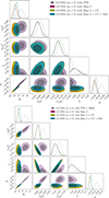Fig. 1. Cosmological parameter constraints for a flat viscous universe with a constant viscosity (m = 0). Top: PPS, Base 2, CC, and R22 datasets. Bottom: PPS + DESI, Base 3, CC, and R22 datasets. Contours show 2D confidence regions (68% and 95% CL) and their 1D marginalized posterior distributions.

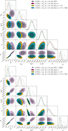Fig. 2. Cosmological parameter constraints for a non-flat viscous universe with constant viscosity (m = 0). Top panel: PPS, Base 2, CC, and R22 datasets. Bottom panel: PPS + DESI, Base 3, CC, and R22 datasets. The contours show 2D confidence regions (68% and 95% CL) and their 1D marginalized posterior distributions.

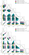Fig. 3. Cosmological parameter constraints for a flat viscous universe with free m. Top panel: PPS, Base 2, CC, and R22 datasets. Bottom panel: PPS + DESI, Base 3, CC, and R22 datasets. Contours show 2D confidence regions (68% and 95% CL) and their 1D marginalized posterior distributions.

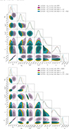Fig. 4. Cosmological parameter constraints for a non-flat viscous universe with m free. Top panel: PPS, Base 2, CC, and R22 datasets. Bottom panel: PPS + DESI, Base 3, CC, and R22 datasets. Contours show 2D confidence regions (68% and 95% CL) and their 1D marginalized posterior distributions.

4.1. m = 0 scenario

We first analyzed the simplest viscous scenario with m = 0, corresponding to a constant bulk viscosity. The resulting constraints are summarized in Table C.1. Both the flat universe (Fig. 1) and the curved universe (Fig. 2) cases exhibit strong positive correlations between H₀ and M (corr > 0.95) across all dataset combinations, as well as a variable correlation with Ω_K0: negligible for PPS alone (corr = 0.009), but moderately negative when including additional constraints (corr ∼ −0.5). In curved models, H₀ exhibits a weaker negative correlation with ${\stackrel{\sim }{\zeta }}_0$, while ${\stackrel{\sim }{\zeta }}_0$ itself correlates positively with Ω_K (e.g., corr = 0.33 for Base 2 + CC + R22, corr = 0.51 for PPS, and corr = 0.27 for PPS + DESI).

Our analysis of the flat universe scenario in Table C.1 shows that Base 1 yields $H_0=67.{94}_{-0.92}^{+0.97}$ km s⁻¹ Mpc⁻¹, while Base 2 produces a higher estimate of $H_0=70.{39}_{-0.73}^{+0.75}$ km s⁻¹ Mpc⁻¹, resulting in a tension of ∼2σ. Notably, Base 3 provides an intermediate constraint of H₀ = 69.53 ± 0.56 km s⁻¹ Mpc⁻¹, which reduces the tension with Base 1 to ∼1.4σ. This trend continues when the CC data is considered. Incorporating the R22 prior reduces these discrepancies to 1.19σ between the Base 1 + CC + R22 and Base 2 + CC + R22 combinations, and to just 0.29σ between the Base 1 + CC + R22 and Base 3 + CC + R22 datasets, yielding

$$\begin{array}{cc}\hfill H_0& =69.{92}_{-0.74}^{+0.71}\mathrm{km}{\mathrm{s}}^{-1}{\mathrm{Mpc}}^{-1}(\mathrm{Base}1+\mathrm{CC}+\mathrm{R}22),\hfill \end{array}$$(39a)

$$\begin{array}{cc}\hfill H_0& =71.{05}_{-0.60}^{+0.62}\mathrm{km}{\mathrm{s}}^{-1}{\mathrm{Mpc}}^{-1}(\mathrm{Base}2+\mathrm{CC}+\mathrm{R}22),\hfill \end{array}$$(39b)

$$\begin{array}{cc}\hfill H_0& =70.{17}_{-0.51}^{+0.49}\mathrm{km}{\mathrm{s}}^{-1}{\mathrm{Mpc}}^{-1}(\mathrm{Base}3+\mathrm{CC}+\mathrm{R}22),\hfill \end{array}$$(39c)

suggesting that both the inclusion of local R22 measurements and DESI data help alleviate the tension between the datasets. In the non-flat scenario, we observe systematically lower estimates of H₀, specifically $H_0=66.1_{-1.1}^{+1.2}$ km s⁻¹ Mpc⁻¹ for Base 1 and H₀ = (66.3 ± 1.1) km s⁻¹ Mpc⁻¹ for Base 1 + CC. However, when we include R22 prior to the Base 2 + CC and Base 3 + CC datasets, the estimates increase to H₀ = (71.06 ± 0.70) km s⁻¹ Mpc⁻¹ and $H_0=(70.{28}_{-0.58}^{+0.60})$ km s⁻¹ Mpc⁻¹, respectively. These values align with those in the flat geometry scenario, with differences smaller than 0.2σ.

We see that the datasets significantly influence the inferred spatial curvature. Incorporating the R22 prior favors a flat universe, yielding

$$\begin{array}{c}\hfill {\mathrm{\Omega }}_{\mathrm{K}0}=0.{049}_{-0.058}^{+0.059}(\mathrm{Base}1+\mathrm{CC}+\mathrm{R}22),\end{array}$$(40)

which is compatible at 1σ with a flat universe. Including the PPS sample further sharpens these constraints, yielding

$$\begin{array}{c}\hfill {\mathrm{\Omega }}_{\mathrm{K}0}=-0.{002}_{-0.053}^{+0.056}(\mathrm{Base}2+\mathrm{CC}+\mathrm{R}22),\end{array}$$(41)

indicating only a 0.04σ deviation from flatness. We further confirm this trend by considering the DESI data, which yield the following results, all fully consistent with a flat universe:

$$\begin{array}{cc}\hfill {\mathrm{\Omega }}_{\mathrm{K}0}& =0.009\pm 0.032(\mathrm{Base}3),\hfill \end{array}$$(42a)

$$\begin{array}{cc}\hfill {\mathrm{\Omega }}_{\mathrm{K}0}& =0.{009}_{-0.031}^{+0.032}(\mathrm{Base}3+\mathrm{CC}),\hfill \end{array}$$(42b)

$$\begin{array}{cc}\hfill {\mathrm{\Omega }}_{\mathrm{K}0}& =-0.{014}_{-0.029}^{+0.030}(\mathrm{Base}3+\mathrm{CC}+\mathrm{R}22).\hfill \end{array}$$(42c)

Even with the inclusion of the R22 prior and DESI data, we observe no significant deviation of ∼0.5σ. In contrast, some datasets without DESI favor Ω_K0 > 0 at more than 2σ, suggesting a moderate preference toward an open universe. For example, the PPS sample alone gives ${\mathrm{\Omega }}_{\mathrm{K}0}=0.{198}_{-0.092}^{+0.092}$ (2.2σ), while Base 1 yields ${\mathrm{\Omega }}_{\mathrm{K}0}=0.{181}_{-0.074}^{+0.073}$ (2.5σ). This tension suggests that local measurements impose stricter constraints on spatial flatness, effectively breaking the geometric degeneracy.

In addition, the dimensionless viscosity coefficient ${\stackrel{\sim }{\zeta }}_0$ shows good agreement with observational data (see Figs. 5 and 6). For both the flat and non-flat scenarios, the present-day bulk viscosity ζ₀, computed via Eq. (15), is approximately

$$\begin{array}{c}\hfill {\zeta }_0\sim {10}^6\mathrm{Pa}\mathrm{s},\end{array}$$(43)

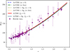Fig. 5. Evolution of Hubble function H(z) with redshift z. Comparison between OHD (purple points with error bars; 0 < z < 2.36) and theoretical predictions. The solid red and green lines corresponds to the ΛCDM and ΛCDM + ΩK models, respectively. The dashed, dash-dotted, and dotted lines correspond to the ΛvCDM and ΛvCDM + ΩK models. The parameters constrained by the Base 2 + CC + R22 dataset.

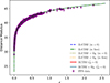Fig. 6. Comparison between the observed distance modulus from PPS compilation (purple points with error bars) within the redshift range 0.001 < z < 2.26 and theoretical predictions. The solid red and green line corresponds to the ΛCDM and ΛCDM + ΩK models, respectively. While the dashed, dash-dotted, and dotted lines represent different cases of the ΛvCDM and ΛvCDM + ΩK models. The parameters constrained by the Base 2 + CC + R22 dataset.

in line with estimates from previous studies (Normann & Brevik 2017; Cruz et al. 2022b). This value is consistent with studies that consider only the isotropic and homogeneous background, which allows for relatively large bulk viscosities without significantly altering the overall expansion history. In particular, Velten & Schwarz (2012) found that viscous dark matter is permitted to have a bulk viscosity up to ζ₀ ∼ 10⁷ Pa s at the background level. However, including bulk viscosity effects on the linear growth of dark matter perturbations leads to much tighter constraints. The effective sound speed, defined as $c_{\mathrm{eff}}^2=\delta \mathrm{\Pi }/\delta \rho$, introduces additional scale-dependent damping terms in the perturbation equations. These terms lead to a strong suppression of small-scale structure formation, yielding constraints as stringent as ζ₀ ≲ 10⁻³ Pa s when both the linear and nonlinear perturbations are considered (Velten & Schwarz 2012; Velten et al. 2014).

Notably, using PPS data alone yields ${\zeta }_0=(0.{72}_{-0.72}^{+1.35})\times {10}^6$ Pa s for the flat geometry, with the lower uncertainty bound approaching zero viscosity (ζ₀ → 0). We observe the same behavior when combining PPS with the DESI dataset, which gives ${\zeta }_0=(0.{47}_{-0.47}^{+0.89})\times {10}^6$ Pa s. In contrast, non-flat scenarios produce significantly higher values: ${\zeta }_0=(2.{04}_{-1.99}^{+3.46})\times {10}^6$ Pa s (PPS) and ${\zeta }_0=(7.{46}_{-3.64}^{+3.60})\times {10}^6$ Pa s (Base 1). When combining both SH0ES calibration into PP (PPS) and the R22 prior, we obtain ${\zeta }_0=(3.{16}_{-2.43}^{+3.17})\times {10}^6$ Pa s in alignment with the results from the flat-case analysis. This pattern suggests that local measurements may indirectly constrain viscous effects in cosmic expansion.

4.2. Free m scenario

We extend our analysis to the more general case, where m is treated as a free parameter. Using the observational datasets Base 1, Base 2, and Base 3, combined with CC data and the R22 prior, we constrained both the flat and non-flat scenarios. The results are summarized in Table C.2 at the 68% CL. Additionally, we present the parameter constraints in Fig. 3 (flat universe) and Fig. 4 (curved universe), which display 2D confidence contours at 68% and 95% CL, as well as the corresponding 1D marginalized posterior distributions for the free parameters (see Table 1).

As in the m = 0 case, Table C.2 shows that the datasets significantly affect the constraints on spatial curvature. The PPS sample alone does not place tight limits on the curvature, yielding ${\mathrm{\Omega }}_{\mathrm{K}0}=0.{205}_{-0.094}^{+0.103}$ (1.99σ). This is consistent within 1σ with (Brout et al. 2022), where ${\mathrm{\Omega }}_{\mathrm{K}0}=0.{07}_{-0.13}^{+0.14}$⁴. On the other hand, Base 1 alone shows a mild preference for an open universe, with (${\mathrm{\Omega }}_{\mathrm{K}0}=0.{21}_{-0.12}^{+0.13}$), corresponding to 1.62σ deviation from flatness. However, including the R22 prior restores consistency with spatial flatness within 1σ, yielding

$$\begin{array}{c}\hfill {\mathrm{\Omega }}_{\mathrm{K}0}=0.{026}_{-0.082}^{+0.087}(\mathrm{Base}1+\mathrm{CC}+\mathrm{R}22).\end{array}$$(44)

Further incorporating the PPS sample leads to significantly tighter constraints,

$$\begin{array}{cc}\hfill {\mathrm{\Omega }}_{\mathrm{K}0}& =0.{007}_{-0.077}^{+0.079}(\mathrm{Base}2),\hfill \end{array}$$(45a)

$$\begin{array}{cc}\hfill {\mathrm{\Omega }}_{\mathrm{K}0}& =0.{008}_{-0.081}^{+0.078}(\mathrm{Base}2+\mathrm{CC}).\hfill \end{array}$$(45b)

This behavior persists with the inclusion of DESI data, yielding

$$\begin{array}{cc}\hfill {\mathrm{\Omega }}_{\mathrm{K}0}& =0.{008}_{-0.035}^{+0.037}(\mathrm{Base}3),\hfill \end{array}$$(46a)

$$\begin{array}{cc}\hfill {\mathrm{\Omega }}_{\mathrm{K}0}& =0.{010}_{-0.035}^{+0.036}(\mathrm{Base}3+\mathrm{CC}),\hfill \end{array}$$(46b)

$$\begin{array}{cc}\hfill {\mathrm{\Omega }}_{\mathrm{K}0}& =-0.009\pm 0.032(\mathrm{Base}3+\mathrm{CC}+\mathrm{R}22).\hfill \end{array}$$(46c)

Notably, when treating m as a free parameter in combination with local measurements, we obtain the most stringent curvature constraints, further supporting spatial flatness.

We find that the PPS yields estimates of H₀ consistent with SN calibrations using Cepheids (Brout et al. 2022; Riess et al. 2022) across all scenarios considered. Specifically, for both m = 0 and free m scenarios, using PPS alone, we obtain

$$\begin{array}{cc}\hfill H_0& =73.1\pm 1.1\mathrm{km}{\mathrm{s}}^{-1}{\mathrm{Mpc}}^{-1}(\mathrm{\Lambda }\mathrm{vCDM}),\hfill \end{array}$$(47a)

$$\begin{array}{cc}\hfill H_0& =73.3\pm 1.2\mathrm{km}{\mathrm{s}}^{-1}{\mathrm{Mpc}}^{-1}(\mathrm{\Lambda }\mathrm{vCDM}+{\mathrm{\Omega }}_{\mathrm{K}}).\hfill \end{array}$$(47b)

Notably, we see no significant shifts in H₀ values between m = 0, free m, and ${\stackrel{\sim }{\zeta }}_0=0$ scenarios across all datasets (see Tables C.1, C.2, and B.1).

Regarding the present-day bulk viscosity, computed from Eq. (15), our results yield a consistent value of ζ₀ ∼ 10⁶ Pa s for both flat and non-flat geometries (analogous to the m = 0 case), in agreement with (Normann & Brevik 2017; Cruz et al. 2022b). In a flat universe, we find a shift toward higher values, ranging from ${\zeta }_0=(0.{51}_{-0.47}^{+1.10})\times {10}^6$ (PPS + DESI) to ${\zeta }_0=(1.{17}_{-1.13}^{+1.87})\times {10}^6$ Pa s (Base 1 + CC), and up to ${\zeta }_0=(1.{97}_{-1.93}^{+2.88})\times {10}^6$ Pa s for Base 2 + CC + R22. Including spatial curvature as a free parameter leads to even higher values, reaching ${\zeta }_0=(8.{03}_{-6.89}^{+8.80})\times {10}^6$ Pa s for Base 1, but decreasing to ${\zeta }_0=(1.{30}_{-1.22}^{+2.73})\times {10}^6$ Pa s for Base 3 + CC + R22. We find that all measured values of the bulk viscosity (ζ₀ > 0) are in full agreement with the second law of thermodynamics. This positivity requirement, ζ₀ ≥ 0 is essential to ensure non-negative entropy production in an expanding universe (Weinberg 1972).

From Figs. 3 and 4, we observe a moderate negative correlation between m and ${\stackrel{\sim }{\zeta }}_0$ (e.g., corr = −0.43 for PPS alone and corr = −0.52 for Base 2 + CC) as well as an anti-correlation between m and Ω_K0 (corr ∼ −0.2 for PPS alone and corr ∼ −0.5 for the other datasets). In contrast, ${\stackrel{\sim }{\zeta }}_0$ and Ω_K0 exhibit a positive correlation (corr ∼ 0.5) across all datasets in the free m case.

Finally, the sign of m in Eqs. (14) and (15) determines the evolution of viscosity. Negative values (m < 0) indicate that viscosity increases as density decreases, meaning it grows with cosmic expansion. In contrast, positive values (m > 0) correspond to viscosity that was stronger in the early Universe and weakens during expansion. The m = 0 case represents constant viscosity. Our results (Table C.2) show that this behavior depends on the dataset. For flat geometry, PPS alone strongly favors m < 0 (e.g., $m=-1.{11}_{-0.82}^{+1.39}$), while several combined datasets yield m > 0, although this trend may change when DESI data are included. A non-flat universe amplifies this effect, driving m to more negative values (e.g., $m=-1.{27}_{-0.72}^{+1.10}$ for PPS alone) and yielding m < −0.4 for Base 1 (+ CC), suggesting curvature-dependent viscous behavior. However, including PPS and the R22 prior shifts m to positive values. On the other hand, when we include DESI data, the results consistently favor m < 0 in both flat and non-flat scenarios, implying that bulk viscosity grows with cosmic expansion.

4.3. Model selection

In the previous sections, we analyzed the observational constraints of various bulk viscous models by computing their respective χ_min² values. To assess their efficiency relative to the ΛCDM model, we evaluate the AIC, BIC, and DIC information criteria as defined in Section 3 (Eqs. (19)–(21)). To complement these criteria, we employ Bayesian evidence, which incorporates prior knowledge for more nuanced model comparisons. In Table D.1, we present the ΔIC values relative to ΛCDM (see Eq. (22)), along with the Bayesian evidence and the Bayes factor for all viscous models.

4.3.1. Information criteria

From Table D.1, we see that both PPS alone and its combinations with DESI data yield ΔAIC < 0 in the four scenarios. For the m = 0 case, the flat scenario yields ΔAIC > 0 for the Base 1 and Base 2 combinations, whereas PPS and the datasets including DESI provide ΔAIC < 0, indicating weak evidence for the ΛCDM model. Specifically, the viscous models show a positive preference with the Base 1(+ CC) datasets. However, this preference diminishes upon incorporating the PPS and R22 prior (e.g., ΔAIC = 1.74 for Base 1 + CC + R22; ΔAIC = 0.62 for Base 2 + CC + R22), but Base 2 alone maintains positive evidence. The ΛvCDM + Ω_K models show stronger evidence arguing against ΛCDM for the Base 1 dataset and positive evidence for the Base 1 + CC dataset. In contrast, the ΛCDM model becomes weakly preferred when either PPS or R22 prior is included (e.g., ΔAIC = −0.90 for Base 1 + CC + R22; ΔAIC = −0.29 for Base 2; ΔAIC = −0.82 for Base 3 and Base 3 + CC). For the free m case, the ΛvCDM models favor the viscous scenario only when using the Base 1 dataset and its combination with CC, with ΔAIC = 6.53 and 6.63, respectively. However, this preference weakens when the R22 prior is included (e.g., ΔAIC = 1.07 for Base 1 + CC + R22) and vanishes when the PPS sample or DESI data are incorporated, for which ΔAIC < 0, indicating a preference for ΛCDM. In contrast, the ΛvCDM + Ω_K models yield ΔAIC > 2 for the Base 1 and Base 2 combinations, whereas including DESI again leads to ΔAIC < 0.

Regarding the BIC, all viscous scenarios yield ΔBIC < 0, favoring the ΛCDM model (see Table D.1). The ΔBIC values impose a strong penalty on viscous models in nearly all cases. For m = 0, the ΛvCDM + Ω_K model yields ΔBIC < −11 when including the R22 prior and PPS, indicating very strong evidence against this curved viscous model. Even without these local measurements, we still find positive evidence against the ΛvCDM + Ω_K models (e.g., ΔBIC = −4.78 with Base 1). For flat scenarios, the Base 2 + CC + R22 constraints provide positive evidence against ΛvCDM (ΔBIC = −4.83), whereas analyses of these priors yield only weak evidence (ΔBIC = −0.84 for Base 1 and ΔBIC = −0.65 for Base 1 + CC). For the free m case, the ΛvCDM + Ω_K model shows very strong evidence against this curved viscous scenario across all datasets (ΔBIC < −11); in particular, ΔBIC = −21.97 for PPS alone. However, this evidence weakens when omitting the local measurements (R22 prior and PPS sample), yielding only positive evidence against the viscous models (ΔBIC = −4.25 for Base 1 and ΔBIC = −4.19 for Base 1 + CC).

The DIC analysis reveals distinct patterns across model configurations. The four scenarios exhibit mixed support depending on the dataset. The flat model with constant viscosity shows values ranging from ΔAIC = −0.6 (PPS) to ΔAIC = 3.31 (Base 1+CC), indicating weak to positive evidence against ΛCDM. In contrast, the curved models show stronger evidence against ΛCDM, particularly for the Base 1 and Base 1 + CC datasets, a pattern that persists when m is free. The inclusion of PPS and R22 prior systematically reduces support for viscous models across all scenarios. Notably, the ΛvCDM + Ω_K model with free m shows the strongest evidence against ΛCDM, reaching ΔDIC = 15.53 for Base 2.

4.3.2. Bayes factor

To complement the information criteria, we also employed Bayesian evidence, which provides more nuanced model comparisons by incorporating prior knowledge. While AIC and BIC apply fixed penalties based on parameter counts, DIC refines this by using the effective number of parameters constrained by the data via posterior distributions, Bayesian evidence inherently penalizes parameters that are unconstrained by data through marginalization over the prior space.

We estimated the natural logarithm of the Bayesian evidence for the bulk viscous models relative to ΛCDM using the MCEvidence code (Heavens et al. 2017a,b)⁵. By reusing existing MCMC chains from parameter inference, we computed Bayes factors for various model-dataset combinations. We interpret the results using the Jeffreys scale (Jeffreys 1961; Kass & Raftery 1995). Different conventions exist for classifying the strength of evidence in the Jeffreys scale, but here we follow the one proposed by Heavens et al. (2017b), as summarized in Table 2.

Following the procedures in the literature (Heavens et al. 2017a,b), we computed lnℬ_0i, where 0 refers to the benchmark ΛCDM model and i indexes each of the four bulk viscous models. The results for all model-dataset combinations are summarized in Table D.1 and calculated as

$$\begin{array}{c}\hfill ln{\mathcal{B}}_{0i}=ln{\mathcal{E}}_{\mathrm{\Lambda }\mathrm{CDM}}-ln{\mathcal{E}}_i.\end{array}$$(48)

From Table D.1, we find moderate evidence against both ΛvCDM + Ω_K scenarios (for both m = 0 and free m cases), with 3 ≤ lnℬ₀₁ < 5 for most datasets. This evidence against models with curvature is particularly strong when we include DESI data, with lnℬ₀₁ > 5 across all datasets. The most disfavored case occurs for m = 0, under the Base 3 + CC + R22 dataset (lnℬ_0i = 7.18). Conversely, the ΛvCDM models with m = 0 show only weak evidence across all datasets (e.g., lnℬ_0i = 1.34 and lnℬ_0i = 1.40 for Base 2 + CC + R22 and Base 2, respectively), while models with free m are inconclusive.

4.4. Evolution of cosmological parameters

Figure 5 shows the evolution of the Hubble parameter as a function of the redshift given in Eq. (13). The model exhibits good agreement with observational Hubble data (OHD; combined CC + BAO + R22 data) at low redshifts (z < 1.5). However, it shows increasing tension with observations at higher redshifts.

The distance modulus for SNe Ia derived from our model is given in Eq. (25). We compared these theoretical predictions with the PPS sample, comprising 1701 light curves from 1550 distinct SNe Ia covering a broad redshift range (see Fig. 6). The model shows good agreement with the observational data.

5. Conclusions

In this work, we carried out an observational analysis of four bulk viscous cosmological models with a cosmological constant, where the bulk viscosity coefficient evolves according to a power law of ζ = ζ₀(Ω_vc/Ω_vc0)^m. We explored both constant viscosity (m = 0) and variable viscosity (m free) scenarios in flat and curved geometries. Using a Bayesian MCMC approach, we constrained these models with Hubble parameter measurements, H(z), from CC and an independent compilation of BAO measurements, BAO data from DESI DR2, SNe Ia data (PP/PPS), and the R22 prior. Our main conclusions are as follows.

The Hubble tension persists; however, it is partially alleviated across all investigated scenarios when local measurements are included. For the flat universe cases, we found $H_0=67.{94}_{-0.92}^{+0.97}$ km s⁻¹ Mpc⁻¹ (Base 1, m = 0), $H_0=70.{39}_{-0.73}^{+0.75}$ km s⁻¹ Mpc⁻¹ (Base 2, m = 0), and H₀ = 69.53 ± 0.56 km s⁻¹ Mpc⁻¹ (Base 3, m = 0). When combining datasets with the R22 prior, the tension reduces to approximately 1σ, yielding $H_0=69.{92}_{-0.74}^{+0.71}$ km s⁻¹ Mpc⁻¹ (Base 1 + CC + R22), $H_0=71.{05}_{-0.60}^{+0.62}$ km s⁻¹ Mpc⁻¹ (Base 2 + CC + R22), and $H_0=70.{17}_{-0.51}^{+0.49}$ km s⁻¹ Mpc⁻¹ (Base 3 + CC + R22). This reduction in tension persists across all tested configurations: spatial geometry (flat/curved), power-law bulk viscosity evolution (m = 0/free m), and null present-day bulk viscosity (${\stackrel{\sim }{\zeta }}_0=0$) scenarios.

For the non-flat scenarios, the models initially favor negative curvature (corresponding to Ω_K0 > 0) at more than 2σ significance in some cases, suggesting a moderate preference for an open universe. However, when the PPS sample and the R22 prior are included, the constraints shift toward spatial flatness (Ω_K0 ≈ 0), consistent within 1σ. This consistency with a flat universe is also achieved, with even tighter uncertainties, when DESI data is incorporated into any of the dataset combinations.

Our results indicate that the present-day bulk viscosity maintains a consistent value of ζ₀ ∼ 10⁶ Pa s across all investigated scenarios. This aligns with the known hierarchy of cosmological constraints, where background expansion permits viscosities several orders of magnitude larger than those allowed by the suppression of small-scale structure formation, as discussed in previous studies (Velten & Schwarz 2012; Velten et al. 2014). Furthermore, the positive values of ζ₀ preferred by our data are physically consistent, satisfying both the second law of thermodynamics within the Eckart framework and remaining compatible with cosmological observations. Specifically, values range from ${\zeta }_0=0.{47}_{-0.47}^{+0.89}\times {10}^6$ Pa s (PPS + DESI, flat case) to ${\zeta }_0=7.{46}_{-3.64}^{+3.60}\times {10}^6$ Pa s (Base 1, non-flat). On the other hand, the viscosity evolution parameter m remains weakly constrained. Using PPS alone favors negative values (m < 0), corresponding to viscosity that increases as density decreases (i.e., growing with cosmic expansion). This preference is also favored by the inclusion of DESI data, which consistently favors m < 0 across both flat and non-flat scenarios, suggesting that bulk viscosity becomes more significant at later times. In contrast, joint analyses without DESI tend to prefer m > 0, indicating that viscosity was more dominant in the early Universe.

Model selection criteria present a nuanced picture. We found that the AIC and DIC criteria favor viscous models in some observational datasets (e.g., ΔAIC > 4 and ΔDIC > 6 for Base 1(+CC)), while the BIC strongly prefers the benchmark ΛCDM model, as it imposes a more severe penalty for additional parameters. We observed that Bayesian evidence calculations further show moderate evidence against non-flat viscous scenarios (3 ≤ lnℬ_0i < 5) for most datasets. This evidence against models with curvature is particularly strong when we include DESI data, with lnℬ_0i > 5 across all datasets. These results suggest that although bulk viscosity can moderately improve cosmological fits, it neither resolves the H₀ tension nor outperforms ΛCDM when local measurements are included.

Our analysis reveals large uncertainties in m and ζ₀ when using H(z) data, SNe Ia samples, and the R22 prior, demonstrating that these datasets cannot definitively distinguish between viscous scenarios. Consequently, the standard ΛCDM model remains the most parsimonious description. Nevertheless, viscous cosmologies still retain significant potential as physically motivated alternative models meriting investigation. To achieve more conclusive results, we aim to extend our investigation to incorporate CMB observations.

Acknowledgments

This research is part of the Ph.D. thesis of R.N. Villalobos and is supported by the Agencia Nacional de Investigación y Desarrollo (ANID) through the Chilean National Doctoral Fellowship N° 21212268. Additionally, this investigation was made possible thanks to funding from the Beca de Arancel y Manutención of the Dirección de Postgrados y Postítulos at the Universidad de La Serena (ULS), along with financial contributions from the Astronomy Doctoral Program at ULS. This work is partially supported by ANID Chile through FONDECYT Grant N° 1220871 (R.N.V. and Y.V.) and FONDECYT Grant No. 1250969 (N.C.). The authors wish to thank the FIULS 2030 project 18ENI2-104235 – CORFO for providing computing resources. We thank the referee for their useful comments and suggestions. Lastly, R.N.V. dedicates this work to their children and Leonardo, whose unwavering love and support have been their strength throughout this academic journey.

References

Appendix A: Observational data

A.1. H(z) data

A.2. DESI data

Appendix B: Case for ${\stackrel{\sim }{\zeta }}_0=0$: ΛCDM model

We conduct a comparative MCMC analysis between the bulk viscous models, ΛvCDM and ΛvCDM + Ω_K, considering both constant (m = 0) and variable viscosity (m free). These models are evaluated against the Benchmark ΛCDM model (with ${\stackrel{\sim }{\zeta }}_0=0$). For quantitative model selection, we compute AIC, BIC, DIC, and lnℰ_i for all models. To ensure transparency, we present the reference ΛCDM results (see Table B.1).

Figure B.1 shows the posterior distributions for the PPS dataset (purple-gray), while Figure B.2 displays the results for the PPS+DESI dataset (purple). Both figures include the confidence regions from our MCMC runs for the other dataset combinations: Base 2, Base 2 + CC, and Base 2 + CC + R22 (dark magenta, green, and sea blue, respectively), alongside their Base 3 counterparts (same color scheme). In all cases, the chains converge rapidly, yielding nearly Gaussian uncertainties.

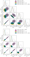Fig. B.1. Cosmological parameter constraints for ΛCDM model with ${\stackrel{\sim }{\zeta }}_0=0$. Top panel: PPS, Base 2, CC, and R22 datasets. Bottom panel: PPS+DESI, Base 3, CC, and R22 datasets. Contours show 2D confidence regions (68% and 95% CL) and their 1D marginalized posterior distributions.

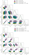Fig. B.2. Cosmological parameter constraints for ΛCDM + ΩK model with ${\stackrel{\sim }{\zeta }}_0=0$. Top panel: PPS, Base 2, CC, and R22 datasets. Bottom panel: PPS+DESI, Base 3, CC, and R22 datasets. Contours show 2D confidence regions (68% and 95% CL) and their 1D marginalized posterior distributions.

Table B.1 summarizes the best-fit parameters along with their 68% CL uncertainties. We adopt the priors listed in Table 1 for the ${\stackrel{\sim }{\zeta }}_0=0$ case, applying Gaussian priors for Ω_dm0h² and Ω_b0h², and uniform priors for the remaining parameters (H₀ and M). We also report results for the curved ΛCDM + Ω_K extension in Table B.1, where we assume a uniform prior for Ω_K0.

We quantify the relative evidence against the benchmark ΛCDM model by computing the following Δ values:

$$\begin{array}{cc}& \mathrm{\Delta }\mathrm{IC}={\mathrm{IC}}_{\mathrm{\Lambda }\mathrm{CDM}}-{\mathrm{IC}}_{\mathrm{\Lambda }\mathrm{CDM}+{\mathrm{\Omega }}_{\mathrm{K}}},\hfill \end{array}$$(B.1)

$$\begin{array}{cc}& ln{\mathcal{B}}_{\mathit{ij}}=ln{\mathcal{E}}_{\mathrm{\Lambda }\mathrm{CDM}}-ln{\mathcal{E}}_{\mathrm{\Lambda }\mathrm{CDM}+{\mathrm{\Omega }}_{\mathrm{K}}}.\hfill \end{array}$$(B.2)

We find that the Base 1 and Base 1 + CC datasets show strong evidence for spatial curvature in information criteria, with ΔAIC > 6 and positive evidence in DIC (e.g., ΔDIC = 5.83 for Base 1 + CC), though their BIC values demonstrate weaker support. Including R22 prior reverses this trend, resulting in negative ΔIC values (ΔAIC = −1.32 for Base 1 + CC + R22; ΔBIC = −6.73; ΔDIC = −0.64). Across all datasets, Bayes factors consistently favor the flat ΛCDM model, reaching maximum evidence for the Base 3+CC+R22 dataset (lnℬ_0i = 4.87).

Appendix C: Summary of cosmological constraints

The cosmological constraints on the parameters: H₀, Ω_K0, Ω_b0h², Ω_vc0h², M, ${\stackrel{\sim }{\zeta }}_0$, and m are summarized in Tables C.1 and C.2.

Appendix D: Model comparison summary

Appendix E: Constraints on H₀ and Ω_K for both bulk viscous and standard models

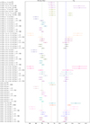Fig. E.1. Whisker plot displaying the 68% marginalized confidence intervals for the Hubble constant H0 (km s−1 Mpc−1) and spatial curvature parameter ΩK, derived from both viscous cold dark matter models with a cosmological constant (ΛvCDM and ΛvCDM+ΩK with m = 0 and free m) and the standard ΛCDM model, including its curved extension. The analysis includes different datasets: DESI, CC, BAO, PP and PPS supernova samples. The red vertical dashed line indicates the H0 measurement from R22 (Riess et al. 2022)), while the blue vertical dashed line marks the ΛCDM prediction for a flat universe (ΩK = 0).

All Tables

All Figures

	Fig. 1. Cosmological parameter constraints for a flat viscous universe with a constant viscosity (m = 0). Top: PPS, Base 2, CC, and R22 datasets. Bottom: PPS + DESI, Base 3, CC, and R22 datasets. Contours show 2D confidence regions (68% and 95% CL) and their 1D marginalized posterior distributions.
In the text

	Fig. 2. Cosmological parameter constraints for a non-flat viscous universe with constant viscosity (m = 0). Top panel: PPS, Base 2, CC, and R22 datasets. Bottom panel: PPS + DESI, Base 3, CC, and R22 datasets. The contours show 2D confidence regions (68% and 95% CL) and their 1D marginalized posterior distributions.
In the text

	Fig. 3. Cosmological parameter constraints for a flat viscous universe with free m. Top panel: PPS, Base 2, CC, and R22 datasets. Bottom panel: PPS + DESI, Base 3, CC, and R22 datasets. Contours show 2D confidence regions (68% and 95% CL) and their 1D marginalized posterior distributions.
In the text

	Fig. 4. Cosmological parameter constraints for a non-flat viscous universe with m free. Top panel: PPS, Base 2, CC, and R22 datasets. Bottom panel: PPS + DESI, Base 3, CC, and R22 datasets. Contours show 2D confidence regions (68% and 95% CL) and their 1D marginalized posterior distributions.
In the text

	Fig. 5. Evolution of Hubble function H(z) with redshift z. Comparison between OHD (purple points with error bars; 0 < z < 2.36) and theoretical predictions. The solid red and green lines corresponds to the ΛCDM and ΛCDM + ΩK models, respectively. The dashed, dash-dotted, and dotted lines correspond to the ΛvCDM and ΛvCDM + ΩK models. The parameters constrained by the Base 2 + CC + R22 dataset.
In the text

Fig. 6. Comparison between the observed distance modulus from PPS compilation (purple points with error bars) within the redshift range 0.001 < z < 2.26 and theoretical predictions. The solid red and green line corresponds to the ΛCDM and ΛCDM + ΩK models, respectively. While the dashed, dash-dotted, and dotted lines represent different cases of the ΛvCDM and ΛvCDM + ΩK models. The parameters constrained by the Base 2 + CC + R22 dataset.

In the text

	Fig. B.1. Cosmological parameter constraints for ΛCDM model with ${\stackrel{\sim }{\zeta }}_0=0$. Top panel: PPS, Base 2, CC, and R22 datasets. Bottom panel: PPS+DESI, Base 3, CC, and R22 datasets. Contours show 2D confidence regions (68% and 95% CL) and their 1D marginalized posterior distributions.
In the text

	Fig. B.2. Cosmological parameter constraints for ΛCDM + ΩK model with ${\stackrel{\sim }{\zeta }}_0=0$. Top panel: PPS, Base 2, CC, and R22 datasets. Bottom panel: PPS+DESI, Base 3, CC, and R22 datasets. Contours show 2D confidence regions (68% and 95% CL) and their 1D marginalized posterior distributions.
In the text

Fig. E.1. Whisker plot displaying the 68% marginalized confidence intervals for the Hubble constant H0 (km s−1 Mpc−1) and spatial curvature parameter ΩK, derived from both viscous cold dark matter models with a cosmological constant (ΛvCDM and ΛvCDM+ΩK with m = 0 and free m) and the standard ΛCDM model, including its curved extension. The analysis includes different datasets: DESI, CC, BAO, PP and PPS supernova samples. The red vertical dashed line indicates the H0 measurement from R22 (Riess et al. 2022)), while the blue vertical dashed line marks the ΛCDM prediction for a flat universe (ΩK = 0).

In the text

References

- Abdul Karim, M., Aguilar, J., Ahlen, S., et al. 2025, Phys. Rev. D, 112, 083515 [Google Scholar]
- Akaike, H. 1974, IEEE Trans. Autom. Control, 19, 716 [Google Scholar]
- Alam, S., Ata, M., Bailey, S., et al. 2017, MNRAS, 470, 2617 [Google Scholar]
- Anand, S., Chaubal, P., Mazumdar, A., & Mohanty, S. 2017, JCAP, 2017, 005 [Google Scholar]
- Anand, S., Chaubal, P., Mazumdar, A., Mohanty, S., & Parashari, P. 2018, JCAP, 2018, 031 [CrossRef] [Google Scholar]
- Anderson, L., Aubourg, É., Bailey, S., et al. 2014a, MNRAS, 441, 24 [Google Scholar]
- Anderson, L., Aubourg, E., Bailey, S., et al. 2014b, MNRAS, 439, 83 [Google Scholar]
- Ashoorioon, A., & Davari, Z. 2023, ApJ, 959, 120 [Google Scholar]
- Avelino, A., & Nucamendi, U. 2010, JCAP, 2010, 009 [Google Scholar]
- Bamba, K., Capozziello, S., Nojiri, S., & Odintsov, S. D. 2012, Ap&SS, 342, 155 [NASA ADS] [CrossRef] [Google Scholar]
- Bautista, J. E., Busca, N. G., Guy, J., et al. 2017, A&A, 603, A12 [NASA ADS] [CrossRef] [EDP Sciences] [Google Scholar]
- Bennett, C. L., Larson, D., Weiland, J. L., et al. 2013, ApJS, 208, 20 [Google Scholar]
- Blake, C., Brough, S., Colless, M., et al. 2012, MNRAS, 425, 405 [Google Scholar]
- Borghi, N., Moresco, M., & Cimatti, A. 2022, ApJ, 928, L4 [NASA ADS] [CrossRef] [Google Scholar]
- Bravo Medina, S., Nowakowski, M., & Batic, D. 2019, Class. Quant. Grav., 36, 215002 [Google Scholar]
- Brout, D., Scolnic, D., Popovic, B., et al. 2022, ApJ, 938, 110 [NASA ADS] [CrossRef] [Google Scholar]
- Caldwell, R. R. 2002, Phys. Lett. B, 545, 23 [Google Scholar]
- Caldwell, R. R., Dave, R., & Steinhardt, P. J. 1998, Phys. Rev. Lett., 80, 1582 [Google Scholar]
- Carroll, S. M. 2001, Liv. Rev. Relat., 4, 1 [NASA ADS] [CrossRef] [Google Scholar]
- Carroll, S. M., Press, W. H., & Turner, E. L. 1992, ARA&A, 30, 499 [NASA ADS] [CrossRef] [Google Scholar]
- Chiba, T. 2002, Phys. Rev. D, 66, 063514 [Google Scholar]
- Chuang, C.-H., & Wang, Y. 2013, MNRAS, 435, 255 [Google Scholar]
- Copeland, E. J., Sami, M., & Tsujikawa, S. 2006, Int. J. Mod. Phys. D, 15, 1753 [NASA ADS] [CrossRef] [Google Scholar]
- Cruz, M., Cruz, N., & Lepe, S. 2017, Phys. Rev. D, 96, 124020 [Google Scholar]
- Cruz, N., González, E., Lepe, S., & Sáez-Chillón Gómez, D. 2018, JCAP, 2018, 017 [CrossRef] [Google Scholar]
- Cruz, N., González, E., & Jovel, J. 2022a, Phys. Rev. D, 105, 024047 [Google Scholar]
- Cruz, N., González, E., & Jovel, J. 2022b, Symmetry, 14, 1866 [Google Scholar]
- Cruz, N., Gómez, G., González, E., Palma, G., & Rincón, Á. 2023, Phys. Dark Univ., 42, 101351 [Google Scholar]
- Delubac, T., Bautista, J. E., Busca, N. G., et al. 2015, A&A, 574, A59 [NASA ADS] [CrossRef] [EDP Sciences] [Google Scholar]
- Di Valentino, E., Ferreira, R. Z., Visinelli, L., & Danielsson, U. 2019, Phys. Dark Univ., 26, 100385 [Google Scholar]
- Di Valentino, E., Mena, O., Pan, S., et al. 2021, Class. Quant. Grav., 38, 153001 [NASA ADS] [CrossRef] [Google Scholar]
- Eckart, C. 1940, Phys. Rev., 58, 919 [Google Scholar]
- Eisenstein, D. J., & Hu, W. 1998, ApJ, 496, 605 [Google Scholar]
- Font-Ribera, A., Kirkby, D., Busca, N., et al. 2014, JCAP, 2014, 027 [Google Scholar]
- Foreman-Mackey, D., Conley, A., Meierjurgen Farr, W., et al. 2013, Astrophysics Source Code Library [record ascl:1303.002] [Google Scholar]
- Frieman, J. A., Turner, M. S., & Huterer, D. 2008, ARA&A, 46, 385 [Google Scholar]
- Fritis, A., Villalobos-Silva, D., Vásquez, Y., López-Caraballo, C. H., & Helo, J. C. 2024, Phys. Dark Univ., 46, 101650 [Google Scholar]
- Gaztañaga, E., Cabré, A., & Hui, L. 2009, MNRAS, 399, 1663 [NASA ADS] [CrossRef] [Google Scholar]
- Heavens, A., Fantaye, Y., Mootoovaloo, A., et al. 2017a, ArXiv e-prints [arXiv:1704.03472] [Google Scholar]
- Heavens, A., Fantaye, Y., Sellentin, E., et al. 2017b, Phys. Rev. Lett., 119, 101301 [Google Scholar]
- Herrera-Zamorano, L., Hernández-Almada, A., & García-Aspeitia, M. A. 2020, Eur. Phys. J. C, 80, 637 [Google Scholar]
- Hinton, S. R. 2016, J. Open Source Softw., 1, 00045 [NASA ADS] [CrossRef] [Google Scholar]
- Israel, W. 1976, Ann. Phys., 100, 310 [Google Scholar]
- Israel, W., & Stewart, J. 1979, Ann. Phys., 118, 341 [CrossRef] [Google Scholar]
- Jeffreys, H. 1961, The Theory of Probability, 3rd edn. (Oxford University Press) [Google Scholar]
- Jiao, K., Borghi, N., Moresco, M., & Zhang, T.-J. 2023, ApJS, 265, 48 [NASA ADS] [CrossRef] [Google Scholar]
- Jimenez, R., & Loeb, A. 2002, ApJ, 573, 37 [NASA ADS] [CrossRef] [Google Scholar]
- Jimenez, R., Verde, L., Treu, T., & Stern, D. 2003, ApJ, 593, 622 [NASA ADS] [CrossRef] [Google Scholar]
- Kass, R. E., & Raftery, A. E. 1995, J. Am. Stat. Assoc., 90, 773 [Google Scholar]
- Komatsu, E., Smith, K. M., Dunkley, J., et al. 2011, ApJS, 192, 18 [Google Scholar]
- Maartens, R. 1995, Class. Quant. Grav., 12, 1455 [Google Scholar]
- Mangano, G., Miele, G., Pastor, S., & Peloso, M. 2002, Phys. Lett. B, 534, 8 [CrossRef] [Google Scholar]
- Mangano, G., Miele, G., Pastor, S., et al. 2005, Nucl. Phys. B, 729, 221 [Google Scholar]
- Moresco, M. 2015, MNRAS, 450, L16 [NASA ADS] [CrossRef] [Google Scholar]
- Moresco, M., Cimatti, A., Jimenez, R., et al. 2012, JCAP, 2012, 006 [CrossRef] [Google Scholar]
- Moresco, M., Pozzetti, L., Cimatti, A., et al. 2016, JCAP, 2016, 014 [CrossRef] [Google Scholar]
- Moresco, M., Amati, L., Amendola, L., et al. 2022, Liv. Rev. Relat., 25, 6 [NASA ADS] [Google Scholar]
- Mörtsell, E., Goobar, A., Johansson, J., & Dhawan, S. 2022, ApJ, 933, 212 [CrossRef] [Google Scholar]
- Normann, B. D., & Brevik, I. 2017, Mod. Phys. Lett. A, 32, 1750026 [Google Scholar]
- Oka, A., Saito, S., Nishimichi, T., Taruya, A., & Yamamoto, K. 2014, MNRAS, 439, 2515 [Google Scholar]
- Padmanabhan, T. 2003, Phys. Rep., 380, 235 [Google Scholar]
- Peebles, P. J., & Ratra, B. 2003, Rev. Mod. Phys., 75, 559 [NASA ADS] [CrossRef] [Google Scholar]
- Perivolaropoulos, L. 2024, Phys. Rev. D, 110, 123518 [Google Scholar]
- Perlmutter, S., Aldering, G., Goldhaber, G., et al. 1999, ApJ, 517, 565 [Google Scholar]
- Planck Collaboration VI. 2020, A&A, 641, A6 [NASA ADS] [CrossRef] [EDP Sciences] [Google Scholar]
- Ratsimbazafy, A. L., Loubser, S. I., Crawford, S. M., et al. 2017, MNRAS, 467, 3239 [NASA ADS] [CrossRef] [Google Scholar]
- Riess, A. G., Filippenko, A. V., Challis, P., et al. 1998, AJ, 116, 1009 [Google Scholar]
- Riess, A. G., Yuan, W., Macri, L. M., et al. 2022, ApJ, 934, L7 [NASA ADS] [CrossRef] [Google Scholar]
- Sanchez, N. G. 2021, Phys. Rev. D, 104, 123517 [Google Scholar]
- Schwarz, G. 1978, Ann. Stat., 6, 461 [Google Scholar]
- Scolnic, D., Brout, D., Carr, A., et al. 2022, ApJ, 938, 113 [NASA ADS] [CrossRef] [Google Scholar]
- Simon, J., Verde, L., & Jimenez, R. 2005, Phys. Rev. D, 71, 123001 [NASA ADS] [CrossRef] [Google Scholar]
- Spiegelhalter, D. J., Best, N. G., Carlin, B. P., & Van Der Linde, A. 2002, J. Roy. Stat. Soc. Ser. B, 64, 583 [Google Scholar]
- Stern, D., Jimenez, R., Verde, L., Kamionkowski, M., & Stanford, S. A. 2010, JCAP, 2010, 008 [Google Scholar]
- Trotta, R. 2008, Contemp. Phys., 49, 71 [Google Scholar]
- Velten, H., & Schwarz, D. J. 2012, Phys. Rev. D, 86, 083501 [Google Scholar]
- Velten, H., Caramês, T. R. P., Fabris, J. C., Casarini, L., & Batista, R. C. 2014, Phys. Rev. D, 90, 123526 [Google Scholar]
- Verde, L., Schöneberg, N., & Gil-Marín, H. 2024, ARA&A, 62, 287 [Google Scholar]
- Wang, Y., Zhao, G.-B., Chuang, C.-H., et al. 2017, MNRAS, 469, 3762 [Google Scholar]
- Wang, D., Zhao, G.-B., Wang, Y., et al. 2018, MNRAS, 477, 1528 [NASA ADS] [Google Scholar]
- Weinberg, S. 1972, Gravitation and Cosmology: Principles and Applications of the General Theory of Relativity (Wiley-VCH) [Google Scholar]
- Weinberg, S. 1989, Rev. Mod. Phys., 61, 1 [NASA ADS] [CrossRef] [Google Scholar]
- Weinberg, D. H., Mortonson, M. J., Eisenstein, D. J., et al. 2013, Phys. Rep., 530, 87 [Google Scholar]
- Yang, W., Pan, S., Di Valentino, E., Paliathanasis, A., & Lu, J. 2019, Phys. Rev. D, 100, 103518 [Google Scholar]
- Zel’dovich, Y. B. 1968, Sov. Phys. Usp., 11, 381 [Google Scholar]
- Zhang, C., Zhang, H., Yuan, S., et al. 2014, RAA, 14, 1221 [NASA ADS] [Google Scholar]
- Zlatev, I., Wang, L., & Steinhardt, P. J. 1999, Phys. Rev. Lett., 82, 896 [Google Scholar]
- Zuntz, J., Paterno, M., Jennings, E., et al. 2015, Astron. Comput., 12, 45 [NASA ADS] [CrossRef] [Google Scholar]
The code is publicly available on https://github.com/yabebalFantaye/MCEvidence