| Issue |
A&A
Volume 708, April 2026
|
|
|---|---|---|
| Article Number | A220 | |
| Number of page(s) | 13 | |
| Section | Extragalactic astronomy | |
| DOI | https://doi.org/10.1051/0004-6361/202556965 | |
| Published online | 08 April 2026 | |
A new sample of faint Blazar cAndidates with Strong opticAl variabiLiTy (BASALT)
1
Dipartimento di Fisica, Università degli Studi di Torino, Via Pietro Giuria 1, 10125 Torino, Italy
2
INAF – Osservatorio Astrofisico di Torino, Via Osservatorio 20, I-10025 Pino Torinese, Italy
★ Corresponding author: This email address is being protected from spambots. You need JavaScript enabled to view it.
Received:
24
August
2025
Accepted:
9
March
2026
Abstract
We present a sample of blazar candidates from the Very Large Array Sky Survey (VLASS) catalog, with cross-referencing to optical and infrared data from the Panoramic Survey Telescope & Rapid Response System (Pan-STARRS) and the Wide-Field Infrared Survey Explorer (WISE), respectively. We focus on compact radio sources and employ a multistage selection process to minimize contamination from non-blazar sources. We considered constraints derived from the radio-optical spectral index and from the infrared and optical colors. We identified the variable objects through an optical variability analysis of Pan-STARRS light curves using two reference samples of stars. We further selected sources whose variability exceeds the level observed in quasars. This led to the selection of 3467 candidates with blazar-like properties and strong optical variability. Only 45% is available in other blazar candidate catalogs, with the remainder representing new identifications. In particular, we unveil a large population of faint sources, down to r ∼ 20.5. The blazar nature of a subsample of these sources is confirmed by available spectra. Our work offers new insights into the blazar population and serves as a foundation for future variability studies, especially in view of the upcoming Legacy Survey of Space and Time at the Vera C. Rubin Observatory, which will reach even fainter sources.
Key words: catalogs / surveys / galaxies: active / BL Lacertae objects: general
© The Authors 2026
 Open Access article, published by EDP Sciences, under the terms of the Creative Commons Attribution License (https://creativecommons.org/licenses/by/4.0), which permits unrestricted use, distribution, and reproduction in any medium, provided the original work is properly cited.
This article is published in open access under the Subscribe to Open model. This email address is being protected from spambots. You need JavaScript enabled to view it. to support open access publication.
1. Introduction
Blazars are a subclass of active galactic nuclei (AGNs) characterized by relativistic jets oriented closely along our line of sight, with consequent Doppler beaming of the jet radiation (Blandford & Königl 1979; Urry & Padovani 1995). Due to their jet-aligned geometry, blazars exhibit extreme observational properties, including rapid variability across the electromagnetic spectrum, high polarization, and significant apparent superluminal motion. In addition, they are characterized by peculiar infrared colors, flat radio spectra, and compact radio morphology (D’Abrusco et al. 2012; Massaro et al. 2013; Xie et al. 2024).
Blazars are typically classified into two main subsets based on their optical spectra: flat-spectrum radio quasars (FSRQs), which usually exhibit prominent broad emission lines typical of quasars, and BL Lacertae objects (BL Lacs), which display weak or no emission lines in their spectra (Stickel et al. 1991; Stocke et al. 1991). This distinction reflects differences not only in the central engines, such as the properties of their accretion disks and surrounding gas, but also in their jet power and radiative efficiencies (e.g., Maraschi et al. 1992; Ghisellini et al. 2014). Flat-spectrum radio quasars tend to exhibit more powerful jets and higher radiative efficiency due to the presence of a luminous accretion disk, while BL Lacs are typically characterized by less powerful jets and lower accretion rates, consistent with a radiatively inefficient accretion flow (e.g., Ghisellini et al. 2011; Sbarrato et al. 2012).
The spectral energy distribution (SED) of blazars is typically double-peaked. The lower-energy peak, which spans radio to X-ray frequencies, is attributed to synchrotron radiation emitted by relativistic electrons within the jet. The higher-energy peak, including X-rays and γ rays, is commonly explained by inverse Compton scattering of soft photons by the same relativistic electrons emitting synchrotron radiation. According to the synchrotron self-Compton (SSC) mechanism, the up-scattered photons are the synchrotron photons themselves (e.g., Ghisellini et al. 2010; Zacharias & Schlickeiser 2012). Although the SSC process is likely sufficient to explain the γ-ray emission in BL Lacs, it generally does not fully account for the emission observed in FSRQs. In these objects, an additional mechanism, external Compton (EC), is likely required (e.g., Abdo et al. 2010). In the EC process, the seed photons originate from external sources, such as the accretion disk, broad line region, or dusty torus, and are subsequently scattered to higher energies by the relativistic jet electrons (e.g., Dermer & Schlickeiser 1993; Sikora 1994; Ghisellini et al. 1998).
Furthermore, hadronic models appear to be an alternative explanation for the high-energy emission in blazars, involving the acceleration of protons and interactions with radiation fields that can end up with particle cascades (e.g., Böttcher et al. 2013). These models, which also predict the production of neutrinos, offer insight into potential connections between blazars and high-energy neutrinos of astrophysical origin detected by neutrino telescopes such as IceCube (e.g., Böttcher 2007; Neronov et al. 2017; Keivani et al. 2018).
Blazar variability can have both an intrinsic and an extrinsic origin. In the first case, flux and polarization changes can be produced by shock waves traveling along the jet (e.g., Marscher & Gear 1985), magnetic reconnection (e.g., Giannios 2013), and turbulence (e.g., Marscher 2014). In the second case, variability is due to changes in jet orientation, with consequent variation in Doppler beaming (e.g., Raiteri et al. 2017).
Blazars, and in particular BL Lacs, represent one of the rarest and most elusive subclasses of AGNs. In the Fermi era, where gamma-ray observations have become a key tool in AGN studies, the need for a reliable, well-classified blazar catalog became increasingly crucial. In this scenario, the Roma-BZCAT catalog1 (Massaro et al. 2009, 2015) was developed as a curated collection of confirmed blazars reported in the literature. Roma-BZCAT contains 3561 sources, divided into five categories: BL Lacs, BL Lac candidates, galaxy-dominated BL Lacs, FSRQs, and blazars of uncertain type. The uncertain category includes objects that exhibit intermittent blazar-like features, such as occasional broad spectral lines or characteristics resembling both BL Lacs and radio galaxies. The catalog classification criteria rely heavily on the distinctive spectral properties of blazars, such as strong nonthermal emission and flat or inverted radio spectra, making Roma-BZCAT a reliable source for high-confidence blazar selection. These criteria align closely with our own selection goals, focusing on well-defined spectral and variability traits that differentiate blazars from other AGNs.
In addition to Roma-BZCAT, several other catalogs of blazars and blazar candidates exist in the literature, each with distinct selection criteria. The Blazar Radio and Optical Survey (BROS) catalog (Itoh et al. 2020) focuses on flat-spectrum radio sources selected from radio and optical surveys, while the Candidate RASS AGN from The Edge Survey (CRATES Healey et al. 2007), identifies blazar candidates through flat radio spectra and ROSAT X-ray counterparts. Other catalogs include the 3HSP catalog (Chang et al. 2019), which identifies high-synchrotron-peaked blazars based on mid-infrared and radio flux ratios, and the ALMA catalog (Paggi et al. 2020), which focuses on blazars observed in millimeter and submillimeter wavelengths using the Atacama Large Millimeter/submillimeter Array (ALMA). Each of these catalogs provides valuable insight and also highlights the need for a systematic multiwavelength approach.
Among these, BZCAT was chosen as our primary reference because of its rigorous verification process, which reduces classification uncertainties and makes it an ideal benchmark for cross-referencing with data at other wavelengths. To have an even more accurate reference sample, we excluded uncertain-type blazars and galaxy-dominated BL Lacs, resulting in a sample of 3060 blazars (with 1059 BL Lacs, 92 BL Lac candidates, and 1909 FSRQs) for a cleaner and more consistent comparison. These are divided into FSRQs and BL Lacs, reported as BZQs and BZBs, respectively, in the BZCAT catalog.
In this paper, we present a new catalog of blazar candidates identified through a broadband analysis. We applied selection criteria based on radio, optical, and infrared source properties. Our methodology exploits the radio compactness, radio-optical spectral index, infrared and optical colors, and variability intensity to distinguish blazar candidates from other radio-loud AGNs. The resulting catalog aims to serve as a valuable resource for future studies, particularly in view of the upcoming Legacy Survey of Space and Time (LSST) at the Vera C. Rubin Observatory, which is expected to significantly improve our understanding of the blazar population through its deep monitoring of the entire southern sky in six bands for ten years (Ivezić et al. 2019; Raiteri et al. 2022).
Our paper is structured as follows. In Sect. 2 we describe the radio data and their use for source selection. In Sect. 3 we present the optical cross-matching procedure and discuss the resulting associations. In Sect. 4 we analyze the infrared and optical colors. Section 5 examines the variability of the candidates. Sections 6 and 7 discuss our final sample in the context of other catalogs and from the perspective of available spectroscopic data. Finally, Sect. 8 explores future prospects and Sect. 9 summarizes our findings, which can be visualized in the flowchart in Fig. 1. Note that for every selection step described in the sections above, we retained at least 95% of the BZCAT sample considered.
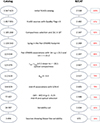 |
Fig. 1. Summary of the sample along the selection steps. The fraction of BZCAT candidates remaining after each cut with respect to the total sample considered is shown in red. |
For the numerical results, we adopt centimeter-gram-second units, unless stated otherwise, and assume a flat cosmological model with parameters H0 = 69.6 km s−1 Mpc−1, ΩM = 0.286, and ΩΛ = 0.714 (Bennett et al. 2014). The optical photometric data used in this work were obtained from the Panoramic Survey Telescope & Rapid Response System (Pan-STARRS; Flewelling et al. 2020) survey, where magnitudes are reported in the AB system (Oke & Schwarzschild 1974; Oke & Gunn 1983). The limiting sensitivity for Pan-STARRS in the r band reaches ∼23 mag. For optical magnitudes we did not apply the correction for Galactic extinction. The radio spectral index is defined as Fν ∝ να.
2. Radio selection of blazars candidates
The selection of blazar candidates begins with data from VLASS, a radio survey covering the sky north of −40 Å declination. Conducted in the 2−4 GHz band, VLASS offers an angular resolution of  , making it well-suited for high-precision studies of radio sources.
The VLASS Epoch 1 Quick Look Catalog version 3, released in September 2023, lists a total of 3 347 423 sources. This update includes an astrometric correction using Gaia positional data, ensuring greater accuracy in source positions (Lacy et al. 2020). The survey achieves a flux sensitivity of approximately 120 μJy per single epoch, with an expected depth of 69 μJy when combining the three planned epochs. However, this release is based on data from a single epoch, as the combined release incorporating multiple epochs is not yet available. Despite this, the high sensitivity of the single-epoch data is already valuable for identifying new blazar candidates, expanding the sample beyond brighter sources cataloged in earlier surveys.
Among the VLASS sources, we aimed to identify and select the radio-compact ones, as radio compactness is a characteristic feature of blazars due to their nuclear-dominated emission – typically confined to small spatial scales, particularly at VLASS’s relatively high frequency (e.g., Liuzzo et al. 2013; Iyida et al. 2021). To assess this source compactness, we considered two morphological parameters:
-
Major axis parameter (Maj): This describes the angular extent of a source along its major axis. Compact sources are expected to have small Maj values.
-
Compactness factor (C): This is defined as C = Stotal/Speak following Itoh et al. (2020), where Speak is the peak flux density and Stotal is the total flux density. Lower values of C indicate more compact morphologies, which align with the typical morphology of blazars.
We did not apply a fixed threshold a priori. Instead, we analyzed the distribution of VLASS sources in the Maj–C diagram in order to choose our selection criteria (see Fig. 2). Only the 1 857 055 sources with reliable flux measurements (i.e., quality flag = 0 in the VLASS catalog) were considered, following the data quality guidelines outlined in Gordon et al. (2021). We also cut off the Galactic plane requiring |b|> 10°. Overall, the VLASS sources exhibit broad dispersion in the Maj and C values.
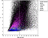 |
Fig. 2. Plot of MaJ vs. C for VLASS sources and those from blazar catalogs. Blazars are mostly located in the bottom-left corner of the diagram, except for BROS sources, which exhibit greater dispersion. |
Instead, when analyzing blazars from the BZCAT catalog (2482 in the VLASS catalog) we observe that these objects are concentrated in the bottom-left portion of the diagram, as expected for compact radio sources. Based on their distribution, we set our selection thresholds to include 97% of the Roma-BZCAT blazars, corresponding to Maj ≤ 7 arcsec and C ≤ 2. The same boundaries apply reasonably well to other catalogs, except for BROS, which shows a broader spread.
It is interesting to explore the properties of the BZCAT sources lying outside the selection region. Visual inspection of these sources identifies two main classes: (1) sources with a core-jet structure (not unexpected for blazars) and (2) bright radio sources in which imaging reconstruction leaves significant contribution from the beam’s sidelobes. In conclusion, we restrict our analysis to the 1 185 268 compact VLASS radio sources, defined as those with Maj ≤7″ and C ≤ 2. These represent about 42% of the original VLASS sample.
3. Optical counterparts of compact radio sources
The first step of our effort to characterize the multiwavelength properties of the compact radio sources found in VLASS focuses on those having optical counterparts in the Panoramic Survey Telescope & Rapid Response System (Pan-STARRS) Catalog. We selected Pan-STARRS because its sky coverage (declination ≳ − 30°) matches VLASS well, and it provides a uniform, deep optical dataset across five broadband filters (g, r, i, z, and y). Its typical single-epoch depth of ∼22 mag in the i band and co-added depth of ∼23.3 mag (Chambers et al. 2016) make it well suited for identifying faint optical counterparts. Moreover, the Pan-STARRS photometric system and depth are comparable to those expected from future surveys such as LSST, making our approach directly relevant to upcoming time-domain and multiwavelength studies (see Sect. 8).
Cross-referencing our VLASS sample with Pan-STARRS serves multiple purposes:
-
Blazar verification: Blazars exhibit distinct optical properties, such as colors and variability, that complement their radio characteristics. Optical counterparts in Pan-STARRS help confirm or support the blazar nature of VLASS sources, improving sample reliability.
-
Multiwavelength characterization: Pan-STARRS optical data enable broader SED analysis and allow us to examine radio-optical continuum properties, such as the broadband spectral index.
-
Minimizing contamination: Requiring Pan-STARRS counterparts removes sources lacking significant optical emission, often unrelated to blazars, such as compact star-forming or dust-obscured galaxies (Calzetti et al. 2000).
Note that, among the 1 185 268 sources selected in Sect. 2, ∼1 130 343 are included in the Pan-STARRS footprint.
3.1. BZCAT-Pan-STARRS association
To identify Pan-STARRS counterparts for BZCAT objects, we first needed to select an appropriate matching radius to ensure accurate cross-identification. To determine this radius, we conducted a simulation by creating 10 000 artificial or “fake” BZCAT catalogs, each with randomized object positions. This methodology follows a similar statistical approach to that adopted for associating Roma-BZCAT sources with SDSS counterparts in Massaro et al. (2014), where mock catalogs were used to quantify the expected rate of random associations and to define a reliable matching radius.
For each fake catalog, we shifted the original positions (right ascension RA, and declination Dec) of the Roma-BZCAT objects by randomly selected offsets. Specifically, we generated random offset distances between 20″ and 30″ and random angles between 0° and 360°. The choice of an offset range ensures that the shifted positions are sufficiently distant from the true sources to avoid accidental real matches, while still remaining within a typical sky area density representative of the environment of the Roma-BZCAT sources. This allows us to estimate the background match rate realistically without introducing bias due to large-scale spatial inhomogeneities (Saxton et al. 2008). The new positions (x and y) were then calculated as follows:

where D is the random offset and θ is the random angle. This transformation assumes a local tangent-plane approximation (i.e., small-angle limit), treating the celestial sphere as flat over arc second-scale displacements. Such an approach is valid and commonly adopted when perturbing positions over small angular scales, where spherical projection effects can be safely neglected.
This simulation allowed us to measure the number of chance (or “mock”) associations within various radii, providing an estimate of the probability of false matches (p-chance) in each radius. Based on this analysis, we found that using a matching radius of  resulted in a p-chance of less than 1%, meaning that fewer than 1% of matches in this radius are expected to be false associations. This low probability of spurious matches indicates that
  is an appropriate and reliable radius for cross-matching BZCAT sources with Pan-STARRS counterparts. Out of the 2347 confirmed BZCAT sources with radio compactness selection outside the Galactic plane, we found 2269 matches in Pan-STARRS. The subset of BZCAT sources with Pan-STARRS counterparts defines our reference sample for identifying blazar candidates via optical colors, variability, and other features.
3.2. VLASS-Pan-STARRS association
By cross-matching our VLASS sample with Pan-STARRS data, we identified optical counterparts for blazar candidates, enabling further analysis of their photometric properties and variability. Given the sub-arcsecond positional accuracy of Pan-STARRS and the  angular resolution of VLASS, a
  cross-match radius offers a good compromise between completeness and reliability in source association. These VLASS sources were not filtered using the duplicate flag < 2 criterion suggested by Gordon et al. (2021) to exclude secondary components or redundant entries. This choice was made to avoid losing real associations since, in preliminary tests, applying this filter reduced the number of matches with confirmed BZCAT blazars by 130. To preserve completeness, we preferred to retain these sources and instead remove redundancy through positional matching.
To ensure the uniqueness of the optical-radio associations, we addressed these cases by selecting only the nearest radio counterpart within the matching radius of  for each Pan-STARRS source. This procedure effectively removes redundant associations caused by duplicate or closely spaced VLASS components linked to the same Pan-STARRS object. However, even after removing multiple associations via nearest-neighbor selection, some VLASS sources in our final sample still have a duplicate flag ≥2. This is because the duplicate flag refers to internal redundancy in the VLASS catalog. This includes multiple radio components of the same physical source or overlapping detections in different survey tiles – not necessarily multiple optical counterparts.
The distribution of optical magnitudes in the matched sources shows a tail at the very faint end (down to r ∼ 29), likely due to photometric uncertainties or spurious detections. To mitigate these effects, we applied magnitude cuts in the g and r bands, keeping only the sources with g < 23.3 and r < 23.2. These limits correspond to the approximate 5σ depth of the Pan-STARRS1 stacked images, as reported by Chambers et al. (2016). At the bright end of the magnitude distribution, we instead set a lower limit at r = 14 and g = 14 to exclude saturated or problematic sources, as described in the Pan-STARRS online documentation2. Magnitude cuts were applied exclusively to the g and r bands, since we used these bands as the basis for subsequent selection steps (see Sects. 3.3 and 4). The number of reliable optical sources found are 223 034 (∼20%).
Another issue with the optical photometric measurements is the presence of extended sources: their photometry is highly uncertain and prone to large scatter in multiple measurements as a result of seeing variations. Furthermore, blazar optical emission, as discussed for the radio band, is compact. We removed extended objects based on the difference between their Kron and point spread function (PSF) magnitude provided by the Pan-STARRS catalog. Following Casadei et al. (2024), we isolated extended objects with rPSF − rKron > 0.3, which can be well separated from point-like sources down to r ∼ 20.5 (see Fig. 3, top panel). The number of compact sources selected by this threshold are 125 070. We applied the same method to the BZCAT sample, finding that the rPSF − rKron > 0.3 requirement excludes 6% of these sources. We note that this criterion may exclude a small fraction of low-redshift blazars whose host galaxy light makes them appear extended in Pan-STARRS images. However, the surface density of such sources is low, and most (such as Mrk 421 and Mrk 501) are well-known objects that have already been extensively observed and classified.
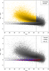 |
Fig. 3. Top: Comparison between the PSF and Kron magnitudes from the Pan-STARRS catalog for the optical counterparts of VLASS compact sources. Their difference is negligible for point sources, while the fluxes of the extended sources are underestimated by PSF photometry. The two groups are well separated using a threshold of rPSF − rKron = 0.3, valid down to r = 20.5. Bottom: Same as the top panel, but with the BZCAT sources highlighted. |
3.3. Radio-Optical spectral index
As a further constraint for selecting blazar candidates, we focus on the radio-to-optical spectral index (αro). The broad spectral range on which αro was estimated reduces the impact of variability-related errors. For our calculation, we used data from VLASS and Pan-STARRS. The optical magnitude in the r band (mr) was converted to optical flux density (Fo) in Janskys (Jy) using the relation: Fo = 3631 × 10−0.4 mr.
The spectral index αro was then computed using
where Fr is the radio flux density and νr and νo are the radio and optical frequencies, respectively. The spectral index distribution of the BZCAT blazars exhibits a bimodal shape (see Fig. 4) with BL Lacs displaying flatter spectral indices than FSRQs. The bimodal behavior reflects the different composition of the two populations, as BL Lacs include a significant fraction of high-energy peaked sources with relatively weaker radio emission compared to FSRQs, leading to systematically different spectral indices (e.g., Padovani & Giommi 1995).
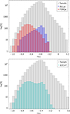 |
Fig. 4. Distribution of the radio–optical spectral index for BZCAT sources and VLASS and Pan-STARRS selected candidates. Top: BZCAT blazar subclasses (BL Lacs and FSRQs), shown separately. Bottom: Distribution for the full BZCAT sample without subclass distinction. |
The VLASS sample distribution of αro shows a broader spread (Fig. 4) and, unlike the BZCAT sample, it does not show a bimodal distribution of spectral indices. The broader spectral index distribution, characterized by a single dominant peak, is likely due to mixing the BL Lac and FSRQ populations – unlike the bimodal behavior observed in the 5BZCAT subsamples when considered separately. Furthermore, one subset of sources shows higher optical flux relative to their radio flux (αro > 0). These sources are likely to be star-forming galaxies, nearby compact FR 0 radio galaxies, or radio-quiet AGNs.
To mitigate their contamination, we then excluded sources with α > −0.3, based on the cumulative distribution of BZCAT. This cutoff corresponds to excluding approximately 2% of the BZCAT FSRQ+BL Lacs sample, ensuring alignment with the known blazar properties while reducing contaminants. Incidentally, this threshold ensures that all the selected sources are radio-loud according to the definition by Kellermann et al. (1989). After applying this criterion, our sample was reduced to 112 624 blazar candidates, which represent ∼90% of the sources selected through the previous steps.
While the α > −0.3 cutoff significantly reduces contamination, a residual overlap with non-blazar populations may persist. Other selection cuts are needed to further refine the sample and ensure greater purity by minimizing the inclusion of non-blazar sources.
4. Infrared selection of blazar candidates
Infrared properties have often been used to select AGNs in general – and blazars in particular (e.g., D’Abrusco et al. 2012; Stern et al. 2012; Assef et al. 2013; Secrest et al. 2015) – including IR-based color-color selections such as those adopted for the 1WHSP sample (Arsioli et al. 2015). To incorporate infrared information, we cross-matched the sample of 112 624 blazar candidates discussed in the previous section with data obtained by the Wide-field Infrared Survey Explorer (WISE; Wright et al. 2010). In particular, we considered unWISE, the catalog of enhanced WISE co-adds that improves the original WISE imaging by using an unblurred point spread function (Lang 2014). We applied a positional tolerance of 3″, following the prescriptions of Raiteri et al. (2014). From the cross-match with the unWISE catalog, we found 110 717 sources, ∼98% of the candidates. We then applied a further cut based on the signal-to-noise ratio in the W1 and W2 data and retained the 104 829 objects with S/N ≥ 3 in both bands.
Several studies have used the W1−W2 versus W2−W3 color-color diagram to select blazars (e.g., Massaro et al. 2011). However, the significantly lower sensitivity and spatial resolution of the W3 data would strongly limit our analysis to the brightest sources. For this reason, we instead produced a W1−W2 versus g − r diagram, including information on both the infrared and optical colors.
To account for Galactic extinction in the optical bands, we corrected the observed g- and r-band magnitudes using the color excess E(B − V) obtained from the IRSA Galactic Dust Reddening and Extinction service3. The extinction coefficients were taken from the recalibrated dust maps of Schlafly & Finkbeiner (2011), which provide the ratios Aλ/E(B − V) for the SDSS filter system. However, these coefficients are known to be very similar to those of the Pan-STARRS photometric system (Tonry et al. 2012). The corrected magnitudes were therefore computed as
where the numerical factors represent the extinction in units of E(B − V) for the corresponding filters. These corrections were applied prior to the construction of the optical color-color diagram used to identify the region of interest in our analysis.
This diagram (see Fig. 5, top panel) reveals a bimodal clustering of sources, with one group in the upper-left and the other in the lower-right portion of the plot. In the bottom panel of Fig. 5, we overlay the distribution of the BZCAT sources: they are mostly confined to the region of high W1−W2 color (≳0.6) and low g − r color (≲0.7). Among these sources, FSQRs generally have redder infrared colors and bluer optical spectra than BL Lacs. The redder infrared colors of the FSRQs arise from stronger synchrotron contribution in that band, while the bluer optical spectra result from the emission contribution from the big blue bump, which is likely due to thermal radiation from the accretion disk and the broad line region (e.g., Raiteri et al. 2014).
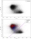 |
Fig. 5. Top: Distribution of the blazar candidates selected through cuts described in previous sections in the W1−W2 vs. g − r color-color diagram. Bottom: BZCAT objects added to the distribution. The BZCAT sources are distinguished by the BL Lac (blue) and FSRQ (red) sources. |
The bimodal distribution of the VLASS sources suggests two distinct populations. Those in the bottom-right portion of the diagram have both infrared and optical colors typical of an evolved stellar population (Wright et al. 2010; Yao et al. 2020), with the dispersion of these sources likely due to a broad range of redshift (Hernández-Yévenes et al. 2024). We can identify this group with the large population of compact radio sources hosted by elliptical galaxies and named FR 0 (Baldi 2023). Indeed, cross-matching with the FR0CAT catalog (Baldi et al. 2018) of compact FR 0 radio galaxies reveals that 92 of the 108 sources overlap with our VLASS sample within a matching radius of  . All of these are located in the bottom-right portion of the W1−W2 versus g − r plane.
The second group by contrast exhibits blazar-like colors. A frequently adopted demarcation to isolate blazars is W1 − W2 > 0.5, widely used in the literature to identify quasar-like AGNs (Stern et al. 2012). However, this boundary does not capture the full distribution of BZCAT sources, as many do not satisfy this criterion. Furthermore, it does not reproduce the bimodality of the VLASS sources. We thus selected a boundary that also considers optical color, empirically derived from the BZCAT and VLASS source distribution:

This cut retains ∼97% of the BZCAT sample, ensuring minimal loss of known blazars while effectively reducing contamination. At this stage, we had 77 007 blazar candidates – about 73% of sources with WISE detections where fluxes have signal-to-noise ratios higher than 3.
5. Optical variability of blazar candidates
5.1. Selection of variable Pan-STARRS sources
For all BZCAT sources and our VLASS-Pan-STARRS sample, we retrieved light curves following the procedure outlined in the Pan-STARRS website4. Most of the optical light curves of Pan-STARRS were derived from the 3π survey, which covered the sky from May 2010 to March 2014. The 3π survey was aimed at observing each field 12 times per filter, on six distinct nights, typically with two visits per night separated by 20−30 minutes. The 5σ single-exposure median limiting magnitudes for the 3π survey (with exposure times of 30 to 45 seconds, depending on the filter) are approximately: 22.1 (g), 21.9 (r), 21.6 (i), 20.9 (z), and 19.9 (y; Morganson et al. 2014). These limits vary modestly depending on observing conditions (e.g., seeing) and sky area.
The output table for each light curve includes flux values (in units of jansky) and their associated errors. To convert these fluxes into magnitudes, we used the formula: mag = −2.5log10(FPSF)+8.90, where FPSF is the calculated PSF flux. To ensure the best possible sampling across the filters, we built composite light curves using all data available in the various bands and converting magnitudes to a common reference filter through average color indexes. Specifically, using the most sampled i filter (see Table 11 in Chambers et al. 2016) as reference, we applied corrections to the magnitudes in other bands as follows:
![Mathematical equation: $$ \begin{aligned} i_{\eta } = \eta +[\mathrm{med} (i) - \mathrm{med} (\eta )], \end{aligned} $$](/articles/aa/full_html/2026/04/aa56965-25/aa56965-25-eq12.gif)
where η represents the magnitude in one of the r, g, z, and y bands, and med is the median value of the corresponding light curve. We refer to iη as the synthetic i-band magnitude derived from the other bands (properly scaled).
Effectively, we assumed identical light curves across the different bands, differing only by a constant value determined on a source-by-source basis. That is, we neglected spectral variations. However, this is expected to be an acceptable approximation for our purposes, which allowed us to generate better-sampled light curves. Furthermore, a quality cut was applied to retain only high-confidence measurements, keeping data points with the quality flag psfQfPerfect > 0.85, corresponding to the PSF model fits with fewer than 15% masked pixels weighted by the PSF (Simm et al. 2015).
While analyzing the light curves, we identified individual photometric measurements that deviated significantly from the general variability trends (see Fig. 6 for an example), a problem that was also highlighted by Simm et al. (2015). These outlier data points could be due to transient data artifacts inherent to the survey and/or underestimated photometric errors. Such artifacts can result in misleadingly precise measurements, producing spurious variability in the light curves.
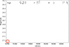 |
Fig. 6. Light curve of one of the objects among the VLASS candidate sample. The red circle highlights a clear outlier that must be removed for accurate variability analysis. |
Addressing this issue required applying robust cleaning methods to the data. This included flagging and excluding suspicious points that could not be confidently attributed to genuine astrophysical variability. The interquartile range (IQR) method, widely used in variability analyses, was applied to identify and remove data points that deviated significantly from the bulk of the distribution (e.g., Sokolovsky et al. 2017). However, it must be applied cautiously to avoid discarding genuine variations.
Specifically, we identified data points lying outside the IQR and applied a criterion to distinguish isolated outliers from potentially significant variations. If one or two points outside the IQR were isolated, they were removed. In contrast, if three or more points outside the IQR were clustered within a temporal range of 5 days or less, they were retained. This approach minimizes the risk of discarding real outbursts or significant variations in the light curves, ensuring a balance between noise removal and preserving astrophysical signals.
To define a robust variability threshold based on Pan-STARRS photometry, we considered a reference sample of field stars. In particular, we used the star catalogs from Xue et al. (2008) and Boyle et al. (1990) and computed the median absolute deviation (MAD) for each light curve (Fig. 7). While we cannot exclude the possibility that some sources in this sample may exhibit low-level intrinsic variability or contain unrecognized outliers, the ensemble represents the typical level of photometric scatter in invariable objects.
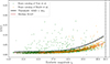 |
Fig. 7. Distribution of MAD as a function of median synthetic magnitude (iη) for stars in the training sample. The dashed red curve shows the median MAD at varying median magnitudes, while the black curve shows the threshold for selecting optically variable sources (i.e., |

We used the MAD because it is a statistical estimator less sensitive to outliers than the classical standard deviation. Specifically, we used σG = 1.4826 × MAD, which provides a consistent estimate of the standard deviation for normally distributed data.
We then analyzed the behavior of MAD as a function of the median magnitude. The reference samples were binned into 0.25 mag intervals for sources with mag < 20.5, and the median MAD was computed for each bin. We excluded fainter sources, because their MAD becomes increasingly dominated by noise, compromising the reliability of the variability threshold. Our analysis was restricted to this well-characterized magnitude range. For each magnitude bin, we defined the threshold for positive variability detection as the median MAD ( ) in that bin plus three times the robust standard deviation:
  . The threshold remains ∼0.01 mag up to iη ∼ 17, then rises rapidly to ∼0.03 mag at iη ∼ 19 and ∼0.1 mag at iη ∼ 20.5. We fitted the thresholds measured in each bin with a fourth-order polynomial law.
A source in the VLASS–Pan-STARRS sample was classified as variable if its MAD exceeded the threshold corresponding to its median magnitude. This approach ensured a data-driven classification of variability, avoiding extrapolation into low-S/N regions while minimizing the impact of outliers and non-Gaussian noise in the photometric data.
Applying the variability selection criterion described above to the VLASS–Pan-STARRS sample (see Fig. 8), we identified 24 997 variable sources. These objects exhibit statistically significant deviations from the expected photometric scatter within their respective magnitude bins. This subset represents the portion of the sample that exhibits variability beyond measurement uncertainties or background noise and thus likely includes sources with genuine astrophysical variability.
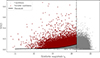 |
Fig. 8. Distribution of MAD as a function of median synthetic magnitude for the compact VLASS sources with a Pan-STARRS counterpart. The thick black curve shows the threshold selected for variable optical sources. |
5.2. Selection of sources with blazar-like variability
The selection criteria filtered radio-loud sources with compact radio and optical emission, blue optical and a red infrared continuum, and significantly variable optical emission. However, this strategy does not ensure that all selected sources are blazars. In fact, radio-loud quasi-stellar objects (QSO) – not necessarily blazars – fulfill all these criteria. In particular, variability is commonly observed in QSOs (see, for example, Netzer & Peterson 1997), associated with changes in accretion rate and disk structure.
To isolate sources whose variability exceeds the level typical of QSOs, we considered the catalog of 750 414 quasars from the Sloan Digital Sky Survey (SDSS; York et al. 2000), data release 16 (DR16; Lyke et al. 2020). We restricted the analysis to the QSOs undetected in the radio band by FIRST to exclude radio-loud sources – among which FSRQs can be present – and applied the same optical-infrared color filter described in Sect. 4.
On the 637 220 selected sources, we applied the same method to inspect their Pan-STARRS light curve variability, as used for the VLASS sources. Following the strategy used to assess stellar variability, we measured MAD for all QSOs. Within each bin, spanning 0.25 magnitudes, we estimated the median MAD and its 3σ level. We adopted the same threshold as before to produce a sample with the smallest possible fraction of interlopers. Again, we reproduced the relation between magnitude and MAD with a fourth-order polynomial law (see Fig. 9).
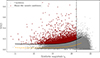 |
Fig. 9. Distribution of MAD for the VLASS-Pan-STARRS sample. We plot MAD as a function of median magnitude for the QSOs in the SDSS DR16 catalog (orange curve) and the |

The  threshold starts at ∼0.15 magnitudes; however, at iη ∼ 18 it rises to ∼0.2 magnitudes reaching iη = 20.5. This threshold significantly exceeds that set by the pure photometric capabilities of Pan-STARRS, as determined from our analysis of the two samples of stars. The QSO variability can be interpreted as nearly constant and, when combined with photometric uncertainties, rises for the faintest sources.
In Fig. 9 we show the MAD distribution for the VLASS–Pan-STARRS sample, reporting the median MAD value for the QSOs and the blazar-like variability threshold. A source was classified as showing blazar-like variability when its MAD exceeded the threshold defined by the general population of QSOs. The number of sources selected with this method is 3496. In Table A.1 we report the main properties of ten of these blazar candidates. The full table is available online.
5.3. Pan-STARRS optical variability of BZCAT sources
We also investigated the variability of sources cross-matched with the BZCAT blazar catalog (see Fig. 10). We found that approximately 85% of the 1948 BZCAT sources in the remaining sample exhibit significant variability according to the criterion defined in Sect. 5.1. Among these, 662 are BL Lac objects and 992 are FSRQs. However, after applying the stricter selection criteria described in Sect. 5.2, the number of retained sources dropped to 672, 364 BL Lacs and 308 FSRQs.
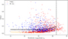 |
Fig. 10. Distribution of MAD for the quasar and BZCAT sample. We also plot MAD as a function of median magnitude for the QSOs in the SDSS DR16 catalog (orange curve) and the |

Several factors may account for the relatively small fraction (26%) of BZCAT blazars found to exhibit blazar-like variability based on our criteria:
-
Low-amplitude optical variability: Some blazars may exhibit only mild flux variations in the optical band, particularly during “quiescent states” when the jet contribution is weak. In such cases, variability can fall below our detection threshold.
-
Big-blue-bump dominance: In some FSRQs the contribution of the big blue bump can dominate the optical emission, making their variability more quasar-like than blazar-like.
-
Insufficient temporal sampling: Rapid, short-duration flares or longer timescale variations that fall between observation epochs might not be captured due to Pan-STARRS cadence.
6. Comparison with blazar catalogues
To assess the reliability and completeness of our sample, we compared our final list of strongly variable sources with several well-known blazar catalogs already presented in Sect. 1: CRATES, BROS, 3HSP, and ALMA, which have a total of 14 467, 88 211, 2013, and 1580 objects respectively. Cross-matching our final sample within a radius of  , we found:
-
903 sources in common with CRATES;
-
1032 sources in common with BROS;
-
200 sources in common with 3HSP;
-
102 sources in common with ALMA.
The comparison revealed that about 30% of our sources are already present in BROS and CRATES, while 3% and 6% are present in ALMA and 3HSP catalogs, respectively. The overall fraction, considering all previous samples combined is ∼35%. This low degree of overlap can be attributed to several factors, including differences in selection criteria and sky coverage. Both BROS and CRATES rely on radio data that are not contemporaneous with VLASS, and their selection criteria are based on different methods that might include a higher level of contamination, particularly from sources such as compact radio galaxies and star-forming galaxies. Furthermore, the sky coverage of these catalogs is also different; for example, CRATES and 3HSP cover the entire sky, while ALMA covers specific regions that do not completely overlap with the VLASS footprint. This, combined with the lack of multiwavelength integration, makes these catalogs more prone to misclassification. In contrast, our approach, which uses high-resolution VLASS data in combination with optical and infrared data from Pan-STARRS and WISE, offers a more comprehensive and up-to-date methodology for selecting blazar candidates. This results in a more stringent selection process that effectively minimizes contamination and provides a more reliable blazar catalog.
To assess how our candidate variable sources relate to known blazars, we also cross-matched them with BZCAT. Out of 3496 candidate sources, 701 are already listed in the BZCAT catalog. In particular, 366 are classified as BL Lac objects, 310 as FSRQs, and 25 as uncertain type.
In conclusion, 1987 sources in our sample (57%) are not listed in any of the above catalogs, including CRATES, BROS, 3HSP, ALMA, and BZCAT. These represent new candidates blazars found by our methodology.
In Fig. 11 we show the magnitude distribution of our candidates (in gray), overlaid with the distributions of the matched BZCAT sources, separately for BL Lacs (blue) and FSRQs (light red, shown with transparency). This histogram demonstrates that (1) up to r ∼ 18 we recover most of the already known BZCAT blazars and (2) at fainter magnitudes only a minority of our candidates are previously known blazars.
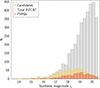 |
Fig. 11. Histogram of the optical magnitude for our blazar candidates (gray) compared to BZCAT-matched sources (yellow), inclduing FSRQs (light red; partially overlapping with BZCAT due to transparency). Only a subset of the candidates is already known as blazars. The BZCAT sources peak at around iη ∼ 18 − 19, while the candidate sample extends to significantly fainter magnitudes at iη ∼ 20. |
Moreover, we cross-matched our candidate catalog with the Fermi-LAT Fourth Source Catalog (4FGL) to identify gamma-ray counterparts and assess the blazar content of our sample. The positional uncertainties of the 4FGL sources were modeled as elliptical confidence regions, with position angles defined from celestial north toward increasing right ascension (eastward), following the catalog convention. An elliptical cross-matching procedure was applied. Using the 86% confidence semimajor and semiminor axes of the 4FGL error ellipses, we identified 680 common sources. Among these, five objects are not classified as blazars in the 4FGL catalog, while 35 sources remain unclassified, resulting in a final sample of 640 blazar associations. Adopting the larger 95% confidence regions increased the number of matched sources to 957, of which 891 are classified as blazars and 60 are unclassified. The remaining sources belong to other AGN subclasses or different source populations.
7. Identification of faint blazar candidates
The results presented above indicate that our method enabled the identification of a significant number of faint sources not included in existing blazar catalogs. The high-resolution and high-frequency capabilities of VLASS – features not used in the construction of previous catalogs – allow us to probe a fainter and more compact radio population, extending beyond the traditional selection regimes.
In particular, BZCAT sources show a broad distribution of optical magnitudes, peaking at iη ∼ 18.5 − 19, with relatively few sources at fainter magnitudes. In contrast, our candidate sample extends down to iη ∼ 20.5, reaching a regime that is underrepresented in current blazar catalogs.
To assess the nature of these faint candidates, we searched for available optical spectra in the Sloan Digital Sky Survey (SDSS). A detailed analysis of these spectra will be presented in a forthcoming study, but here we show two representative examples (Fig. 12). Both sources display blazar-like optical variability and nearly featureless spectra rising toward shorter wavelengths, with no prominent emission or absorption lines. These characteristics are typical of BL Lac objects. These two candidates are among the faintest in our sample, with median synthetic magnitudes of iη = 20.06 and iη = 20.40, respectively.
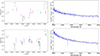 |
Fig. 12. Light curves (left) for two sources showing blazar-like variability selected by our method and their SDSS spectra (right) smoothed with a Gaussian filter with σ = 2 Å. |
8. Future prospects from the Rubin-LSST
The LSST will be conducted by the Vera C. Rubin Observatory and will provide an unprecedented dataset for time-domain astrophysics (Ivezić et al. 2019). It will cover ∼20 000 deg2 of the southern sky in six broad photometric bands (ugrizy), reaching unprecedented depth and temporal resolution. The survey is designed to run for ten years, with observations of the same field typically repeated every ∼3 days. This main observing strategy is referred to as the Wide-Fast-Deep (WFD) survey and is optimized to balance area, depth, and cadence across the extragalactic sky.
LSST capabilities are particularly well suited for studying AGNs, and blazars in particular (Raiteri et al. 2022). In fact, variability-based AGN selection with LSST will be possible down to much fainter magnitudes than current optical surveys, overcoming one of the main limitations in current radio-optical cross-identification efforts. The expected 5σ point-source depth (idealized for stationary sources; Bianco et al. 2022) are

for single visits, and

for co-added images over the ten-year duration of the survey.
In addition to the main WFD survey, LSST will observe a small number of deep drilling fields (DDFs) with significantly increased cadence and depth. These fields, each with a radius of ∼1.75 deg, will receive up to ∼20 000−40 000 visits over the course of the survey, roughly 10−30 times more than typical WFD fields (Bianco et al. 2022). This will enable nightly monitoring in multiple bands, providing densely sampled light curves ideally suited for detecting and characterizing the irregular, stochastic variability of blazars. Moreover, the six-band (ugrizy) photometry will provide crucial color information to separate blazars from contaminant populations such as variable stars and non-blazar AGNs.
As shown in Sect. 3.2, the main limitation of our search for blazars is the relatively low detection rate (∼20%) of optical counterparts for VLASS compact radio sources. This is due to the fact that the sub-millijansky levels reached by the radio surveys include sources that, assuming the typical radio-to-optical emission ratio of blazars, cannot be detected at the Pan-STARRS magnitude threshold. In this context, the LSST DDFs are of particular interest.
The improved depth (down to ∼26 mag) and multiband coverage (ugrizy) of the LSST DDFs will help overcome current limitations such as sparse sampling and reduced photometric precision at faint magnitudes. Furthermore, higher cadence will allow better discrimination between stochastic variability (e.g., AGN) and coherent transients (e.g., flares or microlensing events).
This denser temporal coverage is particularly important for distinguishing blazars from other types of variable sources. Blazars exhibit stochastic, aperiodic variability, characterized by strong color-dependent variability amplitudes and timescales. These statistical properties can be exploited to build robust variability-based selection criteria, especially in the faint regime where color-based selection alone becomes less effective due to larger photometric uncertainties. With LSST, it will be possible to characterize variability parameters with much greater accuracy. This will enable more effective separation of blazars from contaminating populations. Moreover, cross-matching future LSST light curves with existing radio data from VLASS and other surveys will enable multiwavelength studies of variability, contributing to a deeper understanding of the physical mechanisms driving variability in diverse astrophysical populations.
9. Summary and conclusions
In this work, we developed a strategy for the selection of blazar candidates characterized by strong optical variability. Starting from the VLASS radio catalog, we applied several criteria, including radio and optical compactness, the radio-optical spectral index, and optical-infrared characteristics. This selection process involved combining multiwavelength data from VLASS, Pan-STARRS, and WISE to identify blazar candidates while minimizing contamination from non-blazar sources. For each selection step, the thresholds were determined on the basis of the properties of known blazars from the BZCAT catalog, ensuring that our criteria were consistent with established blazar characteristics. A cutoff based on the radio-optical spectral index was applied to exclude potential contaminants such as compact radio galaxies and star-forming galaxies. Additionally, infrared data from WISE were used to further refine our sample and reduce contamination, particularly from elliptical galaxies.
To further refine our selection, optical variability data were incorporated, based on light curves retrieved from Pan-STARRS. The variability patterns of the candidates were examined, focusing on sources that exhibit significant variability consistent with the behavior expected for blazars. We proceeded in two steps: we first assessed the level of variability due to measurement uncertainties and its trend with the magnitude of the source. This was done by using the light curves of two samples of stars observed by Pan-STARRS. We were then in the position of isolating optical variable sources. However, QSOs are also known to be variable sources; thus, variability is not sufficient to select blazars. We thus considered a control sample of radio-quiet QSOs to measure the typical variability level of this population. The 3496 sources showing variability greater that those of QSOs represent our final sample of blazar candidates.
The resulting sample was compared to several existing blazar catalogs, such as CRATES, BROS, 3HSP, ALMA, and BZCAT. Comparing our refined sample with these catalogs reveals low overlap, with a significant portion of our selected candidates (57%, i.e., 1987 sources) absent from them. This likely reflects differences in selection criteria and sky coverage, but primarily the low flux level that can be reached with our analysis.
Indeed, the most important result of this project is the discovery of a large population of previously unknown faint blazars reaching magnitudes as faint as iη ∼ 20.5. Note that in this work, the term “faint” refers to the observed source fluxes, which are close to the sensitivity limits of the optical and radio surveys considered. Disentangling intrinsically low-luminosity blazars from distant, high-redshift objects requires spectroscopic information, which will be explored in a follow-up study. Moreover, in a forthcoming paper we will also consider additional information on the sample of the selected blazar candidates to further explore their nature. These additional data are available only for a fraction of the sources considered here; therefore, we preferred not to select them. However, they can be used to assess, for example, the purity of the sample.
We stress that our selection privileges purity at the expense of completeness: blazars with a very low duty cycle or whose jet emission variability is overwhelmed by a less variable (from the big blue bump) or steady (from the host galaxy) emission contribution escape our variability requirements. The current work provides us with a well-defined catalog of blazar candidates characterized by strongly variable optical emission, offering a solid foundation for future studies on the multiwavelength properties of blazars and their astrophysical significance, issues that will be addressed in a follow up paper. Significant progress in this field is expected from Rubin-LSST. On the one hand, LSST will help us better characterize source variability and further reduce any residual contamination in our sample of candidate blazars. On the other hand, an important limitation of this study is the relatively low fraction (∼20%) of radio sources with an optical counterpart. LSST’s depth improvement over Pan-STARRS, by about 2 magnitudes, will certainly increase this fraction substantially and enable us to explore the population of even fainter blazars.
Data availability
The complete version of Table A.1 is available at the CDS via https://cdsarc.cds.unistra.fr/viz-bin/cat/J/A+A/708/A220
Acknowledgments
C. M. R. and M. I. C. acknowledge financial support from the INAF Fundamental Research Funding Call 2023 (PI: Raiteri). The Pan-STARRS1 Surveys (PS1) and the PS1 public science archive have been made possible through contributions by the Institute for Astronomy, the University of Hawaii, the Pan-STARRS Project Office, the Max-Planck Society and its participating institutes, the Max Planck Institute for Astronomy, Heidelberg and the Max Planck Institute for Extraterrestrial Physics, Garching, The Johns Hopkins University, Durham University, the University of Edinburgh, the Queen’s University Belfast, the Harvard-Smithsonian Center for Astrophysics, the Las Cumbres Observatory Global Telescope Network Incorporated, the National Central University of Taiwan, the Space Telescope Science Institute, the National Aeronautics and Space Administration under Grant No. NNX08AR22G issued through the Planetary Science Division of the NASA Science Mission Directorate, the National Science Foundation Grant No. AST-1238877, the University of Maryland, Eotvos Lorand University (ELTE), the Los Alamos National Laboratory, and the Gordon and Betty Moore Foundation. Funding for the Sloan Digital Sky Survey (SDSS) has been provided by the Alfred P. Sloan Foundation, the Participating Institutions, the National Aeronautics and Space Administration, the National Science Foundation, the U.S. Department of Energy, the Japanese Monbukagakusho, and the Max Planck Society. The SDSS Web site is http://www.sdss.org/. The SDSS is managed by the Astrophysical Research Consortium (ARC) for the Participating Institutions. The Participating Institutions are The University of Chicago, Fermilab, the Institute for Advanced Study, the Japan Participation Group, The Johns Hopkins University, Los Alamos National Laboratory, the Max-Planck-Institute for Astronomy (MPIA), the Max-Planck-Institute for Astrophysics (MPA), New Mexico State University, University of Pittsburgh, Princeton University, the United States Naval Observatory, and the University of Washington. This publication makes use of data products from the Wide-field Infrared Survey Explorer, which is a joint project of the University of California, Los Angeles, and the Jet Propulsion Laboratory/California Institute of Technology, funded by the National Aeronautics and Space Administration. This research has made use of the Astrophysics Data System, funded by NASA under Cooperative Agreement 80NSSC21M00561.
References
- Abdo, A. A., Ackermann, M., Agudo, I., et al. 2010, ApJ, 716, 30 [NASA ADS] [CrossRef] [Google Scholar]
- Arsioli, B., Fraga, B., Giommi, P., Padovani, P., & Marrese, P. M. 2015, A&A, 579, A34 [NASA ADS] [CrossRef] [EDP Sciences] [Google Scholar]
- Assef, R. J., Stern, D., Kochanek, C. S., et al. 2013, ApJ, 772, 26 [Google Scholar]
- Baldi, R. D. 2023, A&ARv, 31, 3 [NASA ADS] [CrossRef] [Google Scholar]
- Baldi, R. D., Capetti, A., & Massaro, F. 2018, A&A, 609, A1 [NASA ADS] [CrossRef] [EDP Sciences] [Google Scholar]
- Bennett, C. L., Larson, D., Weiland, J. L., & Hinshaw, G. 2014, ApJ, 794, 135 [Google Scholar]
- Bianco, F. B., Ivezić, Ž., Jones, R. L., et al. 2022, ApJS, 258, 1 [NASA ADS] [CrossRef] [Google Scholar]
- Blandford, R. D., & Königl, A. 1979, ApJ, 232, 34 [Google Scholar]
- Böttcher, M. 2007, Ap&SS, 309, 95 [CrossRef] [Google Scholar]
- Böttcher, M., Reimer, A., & Zhang, H. 2013, Eur. Phys. J. Web Conf., 61, 05003 [Google Scholar]
- Boyle, B. J., Fong, R., Shanks, T., & Peterson, B. A. 1990, MNRAS, 243, 1 [NASA ADS] [Google Scholar]
- Calzetti, D., Armus, L., Bohlin, R. C., et al. 2000, ApJ, 533, 682 [NASA ADS] [CrossRef] [Google Scholar]
- Casadei, S., Capetti, A., Raiteri, C. M., & Massaro, F. 2024, A&A, 684, A159 [NASA ADS] [CrossRef] [EDP Sciences] [Google Scholar]
- Chambers, K. C., Magnier, E. A., Metcalfe, N., et al. 2016, ArXiv e-prints [arXiv:1612.05560] [Google Scholar]
- Chang, Y. L., Arsioli, B., Giommi, P., Padovani, P., & Brandt, C. H. 2019, A&A, 632, A77 [NASA ADS] [CrossRef] [EDP Sciences] [Google Scholar]
- D’Abrusco, R., Massaro, F., Ajello, M., et al. 2012, ApJ, 748, 68 [CrossRef] [Google Scholar]
- Dermer, C. D., & Schlickeiser, R. 1993, ApJ, 416, 458 [Google Scholar]
- Flewelling, H. A., Magnier, E. A., Chambers, K. C., et al. 2020, ApJS, 251, 7 [NASA ADS] [CrossRef] [Google Scholar]
- Ghisellini, G., Celotti, A., Fossati, G., Maraschi, L., & Comastri, A. 1998, MNRAS, 301, 451 [NASA ADS] [CrossRef] [Google Scholar]
- Ghisellini, G., Tavecchio, F., Foschini, L., et al. 2010, MNRAS, 402, 497 [Google Scholar]
- Ghisellini, G., Tavecchio, F., Foschini, L., & Ghirlanda, G. 2011, MNRAS, 414, 2674 [NASA ADS] [CrossRef] [Google Scholar]
- Ghisellini, G., Tavecchio, F., Maraschi, L., Celotti, A., & Sbarrato, T. 2014, Nature, 515, 376 [NASA ADS] [CrossRef] [Google Scholar]
- Giannios, D. 2013, MNRAS, 431, 355 [NASA ADS] [CrossRef] [Google Scholar]
- Gordon, Y. A., Boyce, M. M., O’Dea, C. P., et al. 2021, ApJS, 255, 30 [NASA ADS] [CrossRef] [Google Scholar]
- Healey, S. E., Romani, R. W., Taylor, G. B., et al. 2007, ApJS, 171, 61 [Google Scholar]
- Hernández-Yévenes, J., Nagar, N., Arratia, V., & Jarrett, T. H. 2024, MNRAS, 531, 4503 [Google Scholar]
- Itoh, R., Utsumi, Y., Inoue, Y., et al. 2020, ApJ, 901, 3 [NASA ADS] [CrossRef] [Google Scholar]
- Ivezić, Ž., Kahn, S. M., Tyson, J. A., et al. 2019, ApJ, 873, 111 [Google Scholar]
- Iyida, E. U., Odo, F. C., & Chukwude, A. E. 2021, Ap&SS, 366, 40 [Google Scholar]
- Keivani, A., Murase, K., Petropoulou, M., et al. 2018, ApJ, 864, 84 [Google Scholar]
- Kellermann, K. I., Sramek, R., Schmidt, M., Shaffer, D. B., & Green, R. 1989, AJ, 98, 1195 [Google Scholar]
- Lacy, M., Baum, S. A., Chandler, C. J., et al. 2020, PASP, 132, 035001 [Google Scholar]
- Lang, D. 2014, AJ, 147, 108 [Google Scholar]
- Liuzzo, E., Giroletti, M., Giovannini, G., et al. 2013, A&A, 560, A23 [NASA ADS] [CrossRef] [EDP Sciences] [Google Scholar]
- Lyke, B. W., Higley, A. N., McLane, J. N., et al. 2020, ApJS, 250, 8 [NASA ADS] [CrossRef] [Google Scholar]
- Maraschi, L., Celotti, A., & Ghisellini, G. 1992, in Physics of Active Galactic Nuclei, eds. W. J. Duschl, & S. J. Wagner, 605 [Google Scholar]
- Marscher, A. P. 2014, ApJ, 780, 87 [Google Scholar]
- Marscher, A. P., & Gear, W. K. 1985, ApJ, 298, 114 [Google Scholar]
- Massaro, E., Giommi, P., Leto, C., et al. 2009, A&A, 495, 691 [CrossRef] [EDP Sciences] [Google Scholar]
- Massaro, F., D’Abrusco, R., Ajello, M., Grindlay, J. E., & Smith, H. A. 2011, ApJ, 740, L48 [NASA ADS] [CrossRef] [Google Scholar]
- Massaro, F., Giroletti, M., Paggi, A., et al. 2013, ApJS, 208, 15 [Google Scholar]
- Massaro, F., Masetti, N., D’Abrusco, R., Paggi, A., & Funk, S. 2014, AJ, 148, 66 [NASA ADS] [CrossRef] [Google Scholar]
- Massaro, E., Maselli, A., Leto, C., et al. 2015, Ap&SS, 357, 75 [Google Scholar]
- Morganson, E., Burgett, W. S., Chambers, K. C., et al. 2014, ApJ, 784, 92 [NASA ADS] [CrossRef] [Google Scholar]
- Neronov, A., Semikoz, D. V., & Ptitsyna, K. 2017, A&A, 603, A135 [NASA ADS] [CrossRef] [EDP Sciences] [Google Scholar]
- Netzer, H., & Peterson, B. M. 1997, Astrophys. Space Sci. Lib., 218, 85 [CrossRef] [Google Scholar]
- Oke, J. B., & Gunn, J. E. 1983, ApJ, 266, 713 [NASA ADS] [CrossRef] [Google Scholar]
- Oke, J. B., & Schwarzschild, M. 1974, Absolute Spectrophotometry in M31 and M32 [Google Scholar]
- Padovani, P., & Giommi, P. 1995, ApJ, 444, 567 [NASA ADS] [CrossRef] [Google Scholar]
- Paggi, A., Bonato, M., Raiteri, C. M., et al. 2020, A&A, 641, A62 [NASA ADS] [CrossRef] [EDP Sciences] [Google Scholar]
- Raiteri, C. M., Villata, M., Carnerero, M. I., et al. 2014, MNRAS, 442, 629 [Google Scholar]
- Raiteri, C. M., Villata, M., Acosta-Pulido, J. A., et al. 2017, Nature, 552, 374 [NASA ADS] [CrossRef] [Google Scholar]
- Raiteri, C. M., Carnerero, M. I., Balmaverde, B., et al. 2022, ApJS, 258, 3 [NASA ADS] [CrossRef] [Google Scholar]
- Saxton, R. D., Read, A. M., Esquej, P., et al. 2008, A&A, 480, 611 [NASA ADS] [CrossRef] [EDP Sciences] [Google Scholar]
- Sbarrato, T., Ghisellini, G., Maraschi, L., & Colpi, M. 2012, MNRAS, 421, 1764 [Google Scholar]
- Schlafly, E. F., & Finkbeiner, D. P. 2011, ApJ, 737, 103 [Google Scholar]
- Secrest, N. J., Dudik, R. P., Dorland, B. N., et al. 2015, ApJS, 221, 12 [NASA ADS] [CrossRef] [Google Scholar]
- Sikora, M. 1994, ApJS, 90, 923 [NASA ADS] [CrossRef] [Google Scholar]
- Simm, T., Saglia, R., Salvato, M., et al. 2015, A&A, 584, A106 [NASA ADS] [CrossRef] [EDP Sciences] [Google Scholar]
- Sokolovsky, K. V., Gavras, P., Karampelas, A., et al. 2017, MNRAS, 464, 274 [CrossRef] [Google Scholar]
- Stern, D., Assef, R. J., Benford, D. J., et al. 2012, ApJ, 753, 30 [Google Scholar]
- Stickel, M., Padovani, P., Urry, C. M., Fried, J. W., & Kuehr, H. 1991, ApJ, 374, 431 [Google Scholar]
- Stocke, J. T., Perlman, E. S., Wurtz, R., & Morris, S. L. 1991, ASP Conf. Ser., 21, 218 [Google Scholar]
- Tonry, J. L., Stubbs, C. W., Lykke, K. R., et al. 2012, ApJ, 750, 99 [Google Scholar]
- Urry, C. M., & Padovani, P. 1995, PASP, 107, 803 [NASA ADS] [CrossRef] [Google Scholar]
- Wright, E. L., Eisenhardt, P. R. M., Mainzer, A. K., et al. 2010, AJ, 140, 1868 [Google Scholar]
- Xie, Z.-L., Bañados, E., Belladitta, S., et al. 2024, ApJ, 964, 98 [Google Scholar]
- Xue, X. X., Rix, H. W., Zhao, G., et al. 2008, ApJ, 684, 1143 [Google Scholar]
- Yao, H. F. M., Jarrett, T. H., Cluver, M. E., et al. 2020, ApJ, 903, 91 [NASA ADS] [CrossRef] [Google Scholar]
- York, D. G., Adelman, J., Anderson, J. E., et al. 2000, AJ, 120, 1579 [Google Scholar]
- Zacharias, M., & Schlickeiser, R. 2012, AIP Conf. Ser., 1505, 660 [Google Scholar]
The online version of Roma-BZCAT is accessible at https://www.ssdc.asi.it/bzcat/
Appendix A: Main properties of the blazar candidates
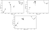 |
Fig. A.1. Example of SEDs of three candidates selected in our final sample. The SEDs have been retrieved using the tool of the Space Science Data Center (SSDC). |
Main properties of the blazar candidates (extract).
All Tables
All Figures
|
Fig. 1. Summary of the sample along the selection steps. The fraction of BZCAT candidates remaining after each cut with respect to the total sample considered is shown in red. |
| In the text | |
|
Fig. 2. Plot of MaJ vs. C for VLASS sources and those from blazar catalogs. Blazars are mostly located in the bottom-left corner of the diagram, except for BROS sources, which exhibit greater dispersion. |
| In the text | |
|
Fig. 3. Top: Comparison between the PSF and Kron magnitudes from the Pan-STARRS catalog for the optical counterparts of VLASS compact sources. Their difference is negligible for point sources, while the fluxes of the extended sources are underestimated by PSF photometry. The two groups are well separated using a threshold of rPSF − rKron = 0.3, valid down to r = 20.5. Bottom: Same as the top panel, but with the BZCAT sources highlighted. |
| In the text | |
|
Fig. 4. Distribution of the radio–optical spectral index for BZCAT sources and VLASS and Pan-STARRS selected candidates. Top: BZCAT blazar subclasses (BL Lacs and FSRQs), shown separately. Bottom: Distribution for the full BZCAT sample without subclass distinction. |
| In the text | |
|
Fig. 5. Top: Distribution of the blazar candidates selected through cuts described in previous sections in the W1−W2 vs. g − r color-color diagram. Bottom: BZCAT objects added to the distribution. The BZCAT sources are distinguished by the BL Lac (blue) and FSRQ (red) sources. |
| In the text | |
|
Fig. 6. Light curve of one of the objects among the VLASS candidate sample. The red circle highlights a clear outlier that must be removed for accurate variability analysis. |
| In the text | |
|
Fig. 7. Distribution of MAD as a function of median synthetic magnitude (iη) for stars in the training sample. The dashed red curve shows the median MAD at varying median magnitudes, while the black curve shows the threshold for selecting optically variable sources (i.e., |
| In the text | |
|
Fig. 8. Distribution of MAD as a function of median synthetic magnitude for the compact VLASS sources with a Pan-STARRS counterpart. The thick black curve shows the threshold selected for variable optical sources. |
| In the text | |
|
Fig. 9. Distribution of MAD for the VLASS-Pan-STARRS sample. We plot MAD as a function of median magnitude for the QSOs in the SDSS DR16 catalog (orange curve) and the |
| In the text | |
|
Fig. 10. Distribution of MAD for the quasar and BZCAT sample. We also plot MAD as a function of median magnitude for the QSOs in the SDSS DR16 catalog (orange curve) and the |
| In the text | |
|
Fig. 11. Histogram of the optical magnitude for our blazar candidates (gray) compared to BZCAT-matched sources (yellow), inclduing FSRQs (light red; partially overlapping with BZCAT due to transparency). Only a subset of the candidates is already known as blazars. The BZCAT sources peak at around iη ∼ 18 − 19, while the candidate sample extends to significantly fainter magnitudes at iη ∼ 20. |
| In the text | |
|
Fig. 12. Light curves (left) for two sources showing blazar-like variability selected by our method and their SDSS spectra (right) smoothed with a Gaussian filter with σ = 2 Å. |
| In the text | |
|
Fig. A.1. Example of SEDs of three candidates selected in our final sample. The SEDs have been retrieved using the tool of the Space Science Data Center (SSDC). |
| In the text | |
Current usage metrics show cumulative count of Article Views (full-text article views including HTML views, PDF and ePub downloads, according to the available data) and Abstracts Views on Vision4Press platform.
Data correspond to usage on the plateform after 2015. The current usage metrics is available 48-96 hours after online publication and is updated daily on week days.
Initial download of the metrics may take a while.