© The Authors 2026

1. Introduction

Gravitational lensing is the effect whereby the path of light is deflected as it travels through the large-scale structure of the Universe. Lensing effects are produced primarily by the distribution of static mass in the Universe; however, the movement of mass induces an additional and, in general, much smaller modulation to the lensing signal. This effect is sometimes referred to as a gravitomagnetic effect (Schäfer & Bartelmann 2006); due to the analogy with the magnetic field within electromagnetism or, alternatively, the frame-dragging potential (Schneider et al. 1992).

This momentum-dependent modulation of gravitational lensing was measured within the Solar System (Fomalont & Kopeikin 2003, Everitt et al. 2011). However, it has not yet been observed on cosmological scales. A measurement of this subtle relativistic effect would provide a manner to directly measure the total matter momentum field (including the dark-matter contribution) and could be used to test Lorentz invariance on cosmological scales.

Gravitational-lensing measurements of the static mass distribution of the Universe provides us with powerful constraints on cosmology through cosmic shear studies (e.g. Wright et al. 2025, Amon et al. 2022, and Dalal et al. 2023) and mass calibration for galaxy-cluster cosmology (e.g. McClintock et al. 2019, Murray et al. 2022, and Bellagamba et al. 2019). However, measuring the momentum field will provide us with complementary information beyond the density field (Cai et al. 2025).

The predicted momentum corrections to lensing are small, of the order of a factor of v/c smaller than the usual lensing effects, where v is the speed of moving mass and c is the speed of light. Therefore, measuring this effect is challenging. The observed convergence field is the sum of two contributions: the density-lensing field sourced by the static mass distribution and the gravitomagnetic lensing field sourced by matter currents. By cross-correlating the total observed lensing signal with a tracer of the momentum field that is uncorrelated with the density lensing field, we can isolate the gravitomagnetic contribution.

In this work, we considered the detectability of gravitomagnetic effects by cross-correlating the lensing field with a reconstructed momentum field estimated from the galaxy overdensity field and compared this to the cross-correlation with the kinetic Sunyaev–Zel’dovich (kSZ) effect field (which also traces the momentum field). We outlined the observational prospects for the first cosmological-scale measurement of this effect.

In Section 2, we give an overview the effects of weak gravitational lensing for moving masses, the kSZ effect, and the angular spectrum of the cosmic momentum field, the cosmic-lensing-momentum field, and the kSZ-field. In Section 3, we present the reconstruction of the cosmological momentum field from the density field of galaxies as well as the reconstruction of the lensing-field from the density field of galaxies. In Section 4, we verify the validity of our predictions using ray-tracing through N-body simulations. In Section 5, we present the detectability of this signal under different observational considerations before concluding in Section 6.

2. Theoretical background

A useful way to conceptualise gravitational lensing is through an analogy with optical refraction, in which we can define an effective index of refraction for a gravitational lens (e.g. Schneider et al. 1992). This analogy is useful provided that the Newtonian gravitational potential, Φ, is small and that the lensing mass distribution is slowly moving. Both of these conditions are generally met on cosmological scales given observed cluster masses (Murray et al. 2022) and cluster velocities (Hand et al. 2012). For a static gravitational potential, the effective index of refraction is

$$\begin{array}{c}\hfill n_{\mathrm{eff}}=1-\frac{2}{c^2}\mathrm{\Phi }.\end{array}$$(1)

To derive the effects of a gravitational lens in motion, we can consider a Lorentz transformation of the optical medium, such that we are in a reference frame with a relative motion with respect to the lens. This provides a direct analogy with the Fizeau experiment (Fizeau 1851), in which the refraction of light by a moving lens was observed. Under this transformation, the effective index of refraction becomes

$$\begin{array}{c}\hfill n_{\mathrm{eff}}=1-\frac{2}{c^2}\mathrm{\Phi }-\frac{4}{c^2}\frac{v_{\Vert }}{c}\mathrm{\Phi },\end{array}$$(2)

where v_∥ is the line-of-sight velocity of the lens. Therefore, the effective index of refraction for a moving lens has a correction factor of $(1+2\frac{v_{\Vert }}{c})$ when compared to the stationary lens. This in turn leads to a correction factor of $(1+2\frac{v_{\Vert }}{c})$ for both the observed deflection angle from a moving lens and its convergence and shear. This equation has been derived in a more formal manner by many authors (e.g. Schneider et al. 1992 and Schäfer & Bartelmann 2006).

2.1. Gravitational lensing from moving masses

From Equation (2), we can derive the weak-lensing convergence in the usual manner, except with a modified source term. Instead of only the matter overdensity, δ, we have the addition of a term proportional to the matter current along the line of sight, j_∥ ≈ δv_∥. Therefore, the weak-lensing convergence, κ, in a flat Universe for a source at a co-moving distance, χ_s, is given by (Schneider et al. 1992)

$$\begin{array}{c}\hfill \kappa (\mathit{\theta },{\chi }_s)=\frac{3H_0^2{\mathrm{\Omega }}_m}{2c^2}{\displaystyle {\int }_0^{{\chi }_s}}d\chi \frac{\chi ({\chi }_s-\chi )}{a(\chi ){\chi }_s}(\delta +\frac{2}{c}{j}_{\Vert }).\end{array}$$(3)

The convergence field can be separated into two terms, κ = κ_Φ + κ_j∥, where κ_Φ is the standard convergence sourced by the static mass distribution, and κ_j∥ is the gravitomagnetic contribution sourced by the line-of-sight momentum field. The lensing kernel as a function of comoving distance, χ, is,

$$\begin{array}{c}\hfill K_{j_{\Vert }}(\chi )=\frac{3H_0^2{\mathrm{\Omega }}_m}{c^3}\frac{\chi ({\chi }_s-\chi )}{a(\chi ){\chi }_s}·\end{array}$$(4)

Therefore, the kernel depends on the geometry of each lens-source system.

2.2. The kinetic Sunyaev–Zel’dovich effect

The kSZ effect (Sunyaev & Zeldovich 1980) provides an independent probe of the line-of-sight momentum field. The kSZ effect occurs when cosmic-microwave-background (CMB) photons Compton-scatter off ionised electrons, which have a net motion with respect to the CMB. This is due to the observed kinematic CMB dipole in the rest frame of the ionised gas. As both the velocity of the ionised gas and the gas density are expected to follow the overall distribution of the matter field, the kSZ effect can be used to measure the projected momentum field. The kSZ effect leads to a temperature change in the CMB of

$$\begin{array}{c}\hfill \frac{\mathrm{\Delta }T}{T_0}(\mathbf{n})=-{\displaystyle \int d}\chi e^{-\tau (\chi )}{\sigma }_T{n}_e(\mathbf{n},\chi )\frac{v_{\Vert }}{c},\end{array}$$(5)

where T₀ is the mean temperature of the CMB; σ_T is the Thomson-scattering cross-section; τ(χ) is the Thomson optical depth to a distance, χ; and n_e is the free electron number density. Assuming that the free electrons trace the matter distribution on large scales, we can relate the electron momentum to the matter momentum field, $n_e{v}_{\Vert }\approx {\overline{n}}_e(z)(v_{\Vert }+j_{\Vert })$. The kSZ kernel is therefore

$$\begin{array}{c}\hfill K_{\mathrm{kSZ}}(\chi )=-\frac{{\sigma }_T{\overline{n}}_e(\chi )e^{-\tau (\chi )}}{c},\end{array}$$(6)

which has a different dependence on the co-moving distance to the lensing kernel in Equation (4).

2.3. The projected cosmic-momentum field

Theoretical predictions for the power spectrum of the momentum field have been studied substantially (Ostriker & Vishniac 1986; Park et al. 2018). To calculate the projected momentum field, the 3D power spectrum of the momentum field, P_q(k, z), is required. It can be shown that this is dominated by the rotational component of the momentum field (e.g. Ma & Fry 2002; Park et al. 2018)¹. The relevant power spectrum is therefore (Ma & Fry 2002; Barrera-Hinojosa et al. 2022)

$$\begin{array}{cc}\hfill P_q(k,z)& ={\displaystyle \int \frac{d^3\mathbf{k}\prime }{{(2\pi )}^3}}(1-{\mu }^2)\hfill \\ \hfill & \times [P_{\delta \delta }(|\mathbf{k}-\mathbf{k}\prime |)P_{\mathit{vv}}(k\prime )-\frac{k\prime }{|\mathbf{k}-\mathbf{k}\prime |}{P}_{\delta v}(|\mathbf{k}-\mathbf{k}\prime |)P_{\delta v}(k\prime )],\hfill \end{array}$$(7)

where $\mu =\widehat{\mathbf{k}}·\widehat{\mathbf{k}\prime }$. In the linear regime, the velocity power spectrum is related to the matter-power spectrum, P_δδ(k), with P_vv(k) = (aHf/k)²P_δδ(k), and the velocity-density cross-power spectrum is P_vδ(k)=(aHf/k)P_δδ(k).

Following Hu (2000) and Ma & Fry (2002), throughout this work we used the non-linear matter power spectrum for density-only terms, while using the linear theory matter-power spectrum for the velocity power spectrum P_vv = (aHf/k)²P_δδ and the density-velocity cross-spectrum $P_{\delta v}=(aHf/k)P_{\delta \delta }^{\mathrm{lin}}$. This is motivated by the 1/k² weighting of the velocity spectrum, which suppresses the impact of non-linear velocity corrections relative to non-linear density corrections (Ma & Fry 2002).

For a given projection kernel, the angular cross-power spectrum of two momentum-dependent observables, A and B, is given by the Limber approximation

$$\begin{array}{c}\hfill C_{\ell }^{\mathit{AB}}={\displaystyle \int d\chi }\frac{K_A(\chi )K_B(\chi )}{{\chi }^2}{P}_{\mathit{AB}}(k=\ell /\chi ,z),\end{array}$$(8)

where the kernel corresponding to the observable of interest can be inserted to get the desired auto- or cross-correlation. The cross-correlation between two observables is greater when the kernels are similar.

3. Reconstructing cosmological fields

In this section, we show how the galaxy density field can be used to reconstruct the momentum field and the lensing field. The interest of the former is clear: by reconstructing this field we can cross-correlate it with the lensing field to isolate the gravitomagnetic-lensing field from the static mass-lensing field. The interest in reconstructing the lensing field is to reduce the variance of the static lensing field on the cross-correlation between the lensing field with the reconstructed momentum field; if this is not yet clear, it should become so in the following sections.

3.1. The cosmic-momentum field

The galaxy overdensity field is defined as ${\delta }_g=n_g/{\overline{n}}_g-1$, where n_g is the number of galaxies in a specified voxel and ${\overline{n}}_g$ is the mean number of galaxies over all of the voxels. Assuming linear biasing of galaxies, this galaxy overdensity field can be related to the underlying matter overdensity field, δ_m:

$$\begin{array}{c}\hfill {\delta }_g=b_g{\delta }_m,\end{array}$$(9)

where b_g is the linear galaxy bias (see Desjacques et al. 2018 for a review on galaxy biasing). Within the standard model of cosmology, velocity perturbations are generated purely from matter perturbations. Within linear theory, we can relate the velocity field to the matter field and in turn substitute the matter density field for the galaxy field using (9); therefore, in Fourier-space,

$$\begin{array}{c}\hfill \widehat{\mathit{v}}{(\mathit{k})}_g=-iaHf\frac{{\delta }_m(k)}{k^2}\mathit{k}=-iaHf\frac{1}{b_g}\frac{{\delta }_g(k)}{k^2}\mathit{k},\end{array}$$(10)

where H is the Hubble equation; f is the linear growth function, which can be written as $f=d\ln \mathrm{D}/\mathrm{d}\ln \mathrm{a}$ where D(a) is the linear growth factor (Kaiser 1987).

The reconstructed momentum field in Fourier-space is

$$\begin{array}{c}\hfill \widehat{\mathit{q}}(k)=\frac{\mathit{iaHf}}{b_g}{\widehat{\delta }}_g(k)\frac{\mathit{k}}{k^2}(1+\frac{{\widehat{\delta }}_g(k)}{b_g});\end{array}$$(11)

here, we write the momentum field in terms of the galaxy density field. Therefore, we were able to estimate the momentum field directly from the galaxy density field. There are many different methods for doing so (e.g. Padmanabhan et al. 2012, White 2015, and Burden et al. 2015). Here, we only considered the simplest method that is valid on linear scales; however, through using non-linear information and the information held within redshift-space distortions the velocity field reconstruction could be performed with lower noise. By then combining the density field with the reconstructed velocity field we can reconstruct the momentum field.

After obtaining the reconstructed momentum field we can project this using Equation (3) to provide a reconstructed gravitomagnetic field for cross-correlation. Importantly we can choose the projection kernel to match that of the observed field in order to maximise the cross-correlation of the fields. The same is not possible for the kSZ field, which is already observed in projection.

The reconstructed momentum field will not be described by the power-spectrum in Equation (7) as the filtering process will change the power-spectrum (Ho et al. 2009). The reconstructed momentum field also contains noise, therefore we need to calculate both the autocorrelation of the reconstructed momentum field and the cross-correlation of the reconstructed momentum field with the true momentum field. Both of these power-spectra are required to estimate the signal-to-noise ratio for the detection of this cross-correlation, as explained in more detail in Section 5.

The Wiener filter is,

$$\begin{array}{c}\hfill W(k)=\frac{b_g^2{P}_m(k)}{b_g^2{P}_m(k)+N(k)}\end{array}$$(12)

where for galaxy surveys, the noise power spectrum is dominated by shot noise,

$$\begin{array}{c}\hfill N(k)=\frac{1}{{\overline{n}}_g(z)}\end{array}$$(13)

where ${\overline{n}}_g(z)$ is the mean number density of galaxies.

Therefore the auto-power spectrum of the reconstructed momentum field is,

$$\begin{array}{cc}\hfill P_{\widehat{q}\widehat{q}}(k,z)& ={\displaystyle \int \frac{d^3\mathbf{k}\prime }{{(2\pi )}^3}}(1-{\mu }^2)b_g^4{W}^4(k)\hfill \\ \hfill & \times [P_{\delta \delta }(|\mathbf{k}-\mathbf{k}\prime |)P_{\mathit{vv}}(k\prime )-\frac{k\prime }{|\mathbf{k}-\mathbf{k}\prime |}{P}_{\delta v}(|\mathbf{k}-\mathbf{k}\prime |)P_{\delta v}(k\prime )],\hfill \end{array}$$(14)

and the cross-power spectrum between the reconstructed momentum field and the true momentum field is,

$$\begin{array}{cc}\hfill P_{\widehat{q}q}(k,z)& ={\displaystyle \int \frac{d^3\mathbf{k}\prime }{{(2\pi )}^3}}(1-{\mu }^2)b_g^2{W}^2(k)\hfill \\ \hfill & \times [P_{\delta \delta }(|\mathbf{k}-\mathbf{k}\prime |)P_{\mathit{vv}}(k\prime )-\frac{k\prime }{|\mathbf{k}-\mathbf{k}\prime |}{P}_{\delta v}(|\mathbf{k}-\mathbf{k}\prime |)P_{\delta v}(k\prime )],\hfill \end{array}$$(15)

Note that in the absence of noise (N → 0), we recover $P_{\widehat{q}q}=P_{\widehat{q}\widehat{q}}=P_{\mathit{qq}}$, where P_qq is given by Equation (7). However, in realistic scenarios, the noise significantly suppresses the reconstructed power on small scales where N ≫ b_g²P_δδ(k, z).

These three-dimensional power spectra can then be projected along the line of sight using the appropriate window functions to obtain the angular correlation functions needed for comparison with lensing observations. The projection integrals involve both the signal and noise contributions from the reconstructed momentum field. We can use Equation (8) to calculate the relevant projected angular correlation functions for the noise fields.

3.2. The cosmic-convergence field

In addition to reconstructing the momentum field, we were also interested in reconstructing the cosmic convergence field. As we explain in Section 5, the primary source of noise for future lensing experiments on the gravitomagnetic-lensing term will be the cosmic variance from the density-convergence field.

In principle, the convergence field can also be estimated from the galaxy overdensity field. We took Equation (3) and ignored the gravitomagnetic contribution, as we only wished to reconstruct the density convergence; we obtained

$$\begin{array}{c}\hfill {\widehat{\kappa }}_{\mathrm{\Phi }}(\mathit{\theta },\chi )=\frac{3H_0^2{\mathrm{\Omega }}_m}{2c^2}{\displaystyle {\int }_0^{\chi }}d{\chi }^{\prime }\frac{{\chi }^{\prime }(\chi -{\chi }^{\prime })}{a({\chi }^{\prime })\chi }{\widehat{\delta }}_g\frac{1}{b_g},\end{array}$$(16)

where once again we simply replaced the matter-density field with the galaxy-density field using the linear galaxy bias relation δ_g = b_gδ_m. This can be then used to subtract the density lensing term from the observed lensing signal. For example, $\kappa -{\widehat{\kappa }}_{\mathrm{\Phi }}$ will have a smaller density-lensing convergence as compared to the directly observed field, κ. However, we see that in practice, even in an idealised case where the galaxy bias is perfectly known, this reconstruction is of limited use.

4. Simulations

The theoretical predictions in the previous section are valid within the linear approximation. However, real cosmological fields are non-linear, particularly on small scales. These non-linearities impact the efficiency of the momentum-field reconstruction and the details of the cross-correlation between the different cosmological fields. To accurately assess these effects and verify that our reconstructed momentum field remains negligibly correlated with the density lensing field even on non-linear scales – a critical requirement for isolating the gravitomagnetic signal – we used N-body simulations. This provides a test to verify that the correlation is insignificant even on non-linear scales, including all the possible contributions from higher order correlations.

In this work, we used the Quijote simulations². These are dark-matter-only N-body simulations; we therefore ignored the important intricacies of the galaxy-halo connection, the halo-matter connection, and baryonic effects. The Quijote simulations provide 512³ particles within a 1000 Mpc/h box, allowing for the sampling of a wide range of scales. We used five different redshift snapshots: z = 0.0, 0.5, 1.0, 2.0, and 3.0.

4.1. Constructing the fields

We used a simplified snapshot geometry (Smith et al. 2018) instead of creating realistic light cones (Breton et al. 2019; Cai et al. 2017; Zhu et al. 2017). Therefore, our setup does not include important light-cone effects; we were nonetheless able to use these fields to confirm the accuracy of our theoretical power spectra and angular-correlation functions.

From the list of particle positions and velocities provided by the simulation snapshots, we constructed 3D grids of matter overdensity, δ, and momentum, q, using a cloud-in-cell mass assignment scheme (implemented within Villaescusa-Navarro 2018)³. From these 3D grids, we calculated 2D fields by projecting along an axis of the box, using the relevant kernel.

For the density convergence field, κ_Φ,

$$\begin{array}{c}\hfill \kappa (\theta )=\frac{3}{2}\frac{H_0^2}{c^2}{\mathrm{\Omega }}_{m,0}{\displaystyle \sum _i}\frac{x_i(x_s-x_i)}{x_s}\delta (x_i).\end{array}$$(17)

For the gravitomagnetic convergence field, κ_j∥,

$$\begin{array}{c}\hfill {\kappa }_{j_{\Vert }}(\theta )=\frac{3H_0^2}{c^3}{\mathrm{\Omega }}_{m,0}{\displaystyle \sum _i}\frac{x_i(x_s-x_i)}{x_s}{j}_{\Vert }(x_i),\end{array}$$(18)

where the sum runs along the specified line of sight. Sub-regions of fields created in this way are shown in Figure 1. There are a couple of interesting points to be noted in this figure. There are overdensities and clear, large positive regions in the density-convergence field where the momentum-convergence field is negative. This is because there are parts of the cosmic web that are moving towards or away from the observer. An overdensity moving away from the observer appears negative in the momentum-convergence field. Conversely, there are underdense (negative κ_Φ) regions in the density convergence that appear positive in the momentum convergence field, κ_∥; these are underdense regions moving away from the observer.

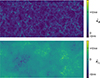Fig. 1. Projected convergence fields constructed from Quijote simulations using a snapshot geometry. Top: Density convergence field, κΦ. Bottom: Momentum convergence field, κ∥. Both images have been smoothed with a Gaussian filter.

4.2. Reconstructed momentum field

We were also able reconstruct the momentum field directly from the density field, without using the particle’s velocity information, in order to mimic the effects of reconstruction where only the galaxy density information is available. This allowed us to verify that the reconstruction method did not introduce a correlation between the density-convergence field and the reconstructed momentum-convergence field, which would complicate the detection of the momentum convergence signal.

The reconstruction procedure was performed as follows:

• We started with the 3D-matter overdensity field δ(x) computed from the simulation snapshot.

• We computed its Fourier transform to obtain δ(k).

• We computed the linear-theory velocity field in Fourier space using Equation (10) and assuming b_g = 1.

• We computed the inverse Fourier transform to obtain $\widehat{v}(\mathit{x}).$

• Finally, we multiplied this by the matter-density field, 1 + δ(x), in order to obtain the reconstructed momentum field, $\widehat{j}(\mathit{x})$.

As before, this-3D reconstructed momentum field was then projected using the gravitomagnetic-lensing kernel (Equation (18)) to provide the reconstructed momentum lensing field ${\widehat{\kappa }}_{j_{\Vert }}$. Therefore, we have two fields in the momentum convergence: essentially κ_j∥ ∼ ∑δv_∥, and the reconstructed momentum convergence ${\widehat{\kappa }}_{j_{\Vert }}\sim {\displaystyle \sum \widehat{\delta }}{\widehat{v}}_{\Vert }$, which is composed of the reconstructed density, $\widehat{\delta }$ (this is exact, but in practice this would be estimated from the galaxy density field) and the reconstructed velocity, $\widehat{v}$.

In Figure 2, we see an excellent agreement between the two fields: the convergence momentum field and the convergence momentum field that has been reconstructed from the density field. In particular, the large-scale features are well reconstructed; however, the small-scale features are different. This is precisely what we would expect in that the large-scales are well described by the linear model in Equation (11) and the small scales become non-linear. Therefore, the approximation of linearity is broken.

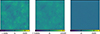Fig. 2. Left: Simulated gravitomagnetic field. Middle: Gravitomagnetic field reconstructed from the density field. Right: Difference between the gravitomagnetic field and the gravitomagnetic field reconstructed from the density field. Both fields were smoothed using a Gaussian filter.

To quantify the quality of the reconstruction and the lack of correlation between the reconstructed momentum convergence field and the density convergence field, we computed the cross-correlation coefficient $r(k)=C_{\mathit{AB}}(k)/\sqrt{C_{\mathit{AA}}(k)C_{\mathit{BB}}(k)}$ for different pairs of projected fields in Fourier space. We performed this analysis for 15 different realisations by using five redshift snapshots and projecting along the three axes of the snapshots for each snapshot. We calculated this for the cross-correlation among the reconstructed momentum convergence field ${\widehat{\kappa }}_{j_{\Vert }}$; the momentum convergence field, κ_j∥; and the density convergence field, κ_ϕ. The results of these cross-correlations are shown in Figure 3. We observe an excellent correlation between the reconstructed momentum convergence field and the true momentum convergence field on large scales. We demonstrate that in this simplified scenario it is possible to accurately reconstruct the gravitomagnetic lensing field from the 3D density field. The correlation rapidly decreases at smaller scales, consistently with the breakdown of the linear theory approximation in our reconstruction method. Importantly, we measure no correlation between the reconstructed momentum convergence field with the density convergence field. This is a crucial result, confirming that our linear reconstruction method does not introduce a spurious correlation with the dominant density lensing signal, thus allowing for a clean isolation of the gravitomagnetic effect. The robustness of this null correlation is a critical requirement for detecting the tiny gravitomagnetic lensing signal, as any leakage from the dominant density convergence could easily overwhelm it.

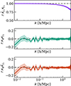Fig. 3. Correlation coefficient r(k) between each of the projected fields. These tests are diagnostics to show that higher order correlations that we did not model do not introduce significant correlations between the density lensing and matter current lensing fields. The solid lines show the mean correlation coefficient from 15 different realisation of the fields (5 snapshots × 3 projection axes), the shaded regions show 1σ error bars calculated from the dispersion of the estimated correlation coefficients. Top: Correlation between the reconstructed momentum convergence, ${\widehat{\kappa }}_{j_{\Vert }}$, and the momentum convergence, κj∥. Middle: Correlation between the momentum convergence, κj∥, and the density convergence, κϕ. Bottom: Correlation between the density convergence, κϕ, and the reconstructed momentum convergence, ${\widehat{\kappa }}_{j_{\Vert }}$.

5. Detection forecasts

Having validated our theoretical framework and confirmed the negligible cross-correlation between the reconstructed momentum field and the density lensing field through simulations, we proceeded to forecast the observational prospects for detecting gravitational lensing induced by cosmological matter currents. This section details the signal-to-noise ratio estimations for various observational configurations.

5.1. Signal-to-noise estimations

The signal-to-noise ratio (S/N) for the cross-power spectra of two Gaussian fields is

$$\begin{array}{c}\hfill {\left(\frac{S}{N}\right)}^2=f_{\mathrm{sky}}{\displaystyle \sum _{\ell }}(2\ell +1)\mathrm{\Delta }\ell \frac{{\left(C^{\mathit{AB}}\right)}^2}{C^A{C}^B+{(C^{\mathit{AB}})}^2},\end{array}$$(19)

where A and B are to be replaced by the field of interest (e.g. κ, κ_j∥, or ${\widehat{\kappa }}_{j_{\Vert }}$). These are the observed power spectra including the noise, and in the following we assume that there is no correlation between the different noise fields and that f_sky is the sky fraction. The power spectra, C, in Equation (19) were obtained from the 3D power spectra using the Limber equation, as detailed in Equation (8).

5.2. Convergence-reconstructed momentum correlations

First we considered the cross-correlation of the lensing convergence with the reconstructed momentum convergence. The results are shown in the left panel of Figure 4. We considered a range of galaxy densities for the reconstruction of the momentum lensing field. These densities range from ${\overline{n}}_g={10}^{-4}$ Mpc⁻³, which is achievable up to high redshifts from current surveys, to ${\overline{n}}_g={10}^{-2}$ Mpc⁻³, which is quite an ambitious value for future spectroscopic galaxy surveys⁴. For the noise on the lensing signal, we considered both stage-four lensing survey noise (Euclid Collaboration: Mellier et al. 2025 and LSST Science Collaboration 2009), which corresponds to a galaxy density of 30 per square arcminute, and cosmic variance noise. In each case, the sky fraction was set to f_sky ≈ 0.25, and the source redshift for lensing was set to z = 2.

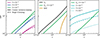Fig. 4. Cumulative S/N forecasts for detecting the gravitomagnetic lensing signal as a function of maximum angular multipole, ℓ. All forecasts assume a sky fraction of fsky ≈ 0.25. Left: S/N for the cross-correlation of the lensing convergence with the reconstructed momentum convergence field for different galaxy number densities (${\overline{n}}_g$, in units of Mpc−3); solid lines show cosmic-variance-limited lensing noise, while dashed lines show stage-four lensing survey noise. Middle: Cosmic-variance-limited S/N for three different momentum field tracers: the true, noiseless field (κj)∥); the reconstructed field (${\widehat{\kappa }}_{j)\Vert }$), assuming a galaxy density of ${\overline{n}}_g={10}^{-2}$ Mpc−3; and the kinetic Sunyaev-Zel’dovich (kSZ) effect. Right: S/N for the cross-correlation after subtracting a reconstructed density convergence field (${\widehat{\kappa }}_{\varphi }$), where the different lines show the effect of varying the galaxy density used for the density reconstruction.

In each of the following we considered the $\mathrm{S}/\mathrm{N}$ for a maximum analysis multipole of ℓ = 5000 and the stage-four lensing noise. On such small scales, we do not expect our theoretical power spectra to be precise, but we were interested in the order of magnitude of the effect as opposed to a precise prediction. The results are as follows:

• For ${\overline{n}}_g={10}^{-4}$ Mpc⁻³, we forecasted a $\mathrm{S}/\mathrm{N}\sim 2.0$; therefore, the effect would not be detectable.

• For ${\overline{n}}_g={10}^{-3}$ Mpc⁻³, the S/N is ∼5.7, which indicates that a statistically significant detection is possible.

• For the ambitious galaxy density of ${\overline{n}}_g={10}^{-2}$ Mpc⁻³, the S/N we achieve is ∼9.5. This would represent a robust, statistically significant detection of the gravitomagnetic lensing signal.

The results for cosmic-variance-limited noise and stage-four lensing noise are similar in our analysis. This is primarily because our current analysis does not consider multiple redshift bins; therefore, the noise on the lensing is principally from the cosmic variance of the density lensing, rather than being shape-noise-limited on most angular scales.

5.3. Cosmic-variance limits

In order to understand the limitations of the detection of the gravitomagnetic lensing field, we considered the cosmic-variance limits for different types of cross-correlations involving tracers of the projected momentum field. These results are shown in the middle panel of Figure 4.

We considered three tracers of the projected momentum field: a noiseless gravitomagnetic field, the reconstructed momentum field (with ${\overline{n}}_g={10}^{-2}$ Mpc⁻³), and the kSZ field. The use of the kSZ field for measuring the gravitomagnetic signal was considered in detail by Barrera-Hinojosa et al. (2022). We found similar results to this work. The kSZ signal, in the presence of the primary CMB, contains signal on small scales. Relatively to the reconstructed momentum field from the galaxy density, we were able to recover the signal on large scales. We see that the reconstructed momentum field approaches a similar S/N to the noiseless momentum field. This is because the noise is primarily from the cosmic-variance contribution from the dominant density lensing field. Therefore, we had to consider how to reduce the impact of the density lensing field.

5.4. Subtracted density convergence: Reconstructed momentum correlations

The detection of this signal is limited by the gravitomagnetic convergence being considerably smaller than the density convergence field. Therefore, ideally we would remove the density convergence field from the observed convergence. In principle, this can be achieved by reconstructing the density convergence field, ${\widehat{\kappa }}_{\varphi }$, and then subtracting this from the observed convergence field, κ.

If this reconstruction were perfect, the resultant field would only contain the momentum convergence contribution. We could then correlate the two fields $\kappa -{\widehat{\kappa }}_{\varphi }$ and ${\widehat{\kappa }}_{j)\Vert }$. This reduces the cosmic-variance contribution from the density convergence to the cross-correlation between the reconstructed momentum and the observed convergence; however, it adds shot noise from the reconstruction of ${\widehat{\kappa }}_{\varphi }$. As described in Section 3.2, we a assumed a simple linear bias and perfect knowledge of the galaxy bias, both of which are unreasonable assumptions.

The results for different galaxy densities in the density convergence reconstruction are shown in the right panel of Figure 4. We can see that on large scales, where the noise is dominated by the cosmic variance from the density lensing, we improved our S/N. On small scales, the S/N decreased as the shot noise from the convergence reconstruction adds more noise to the cross-correlation. Therefore, whilst the improvements were modest at large multipoles, the approach can significantly improve our S/N on linear scales where modelling is easiest.

6. Conclusions

We investigated the prospects for the detection of gravitational lensing induced by cosmological matter currents, a subtle relativistic effect known as gravitomagnetic lensing. Our results show that while measuring this signal is undoubtedly challenging, a statistically significant detection is within reach of upcoming and future cosmological surveys.

The key to isolating this effect, which is typically orders of magnitude smaller than the standard lensing signal from static mass, lies in cross-correlating the total lensing convergence field with a tracer of the large-scale momentum field. We demonstrated, through N-body simulations, that the gravitomagnetic field can be accurately reconstructed from the density field observed in large-scale structure surveys. Crucially, our analysis confirms that this reconstructed momentum field is uncorrelated with the dominant density-lensing signal, a vital condition for a clean measurement. This allows the cross-correlation to effectively filter out the much larger density-lensing contribution, isolating the gravitomagnetic signal.

Our forecasts show that a stage-four CMB-lensing experiment combined with a spectroscopic galaxy survey with a number density of ${\overline{n}}_g={10}^{-3}$ Mpc⁻³ can achieve a detection with a S/N of approximately 5.7. More ambitious surveys could yield an even more robust detection with a S/N approaching 10. We also found that the primary limitation for this measurement is the cosmic variance from the density-lensing field itself. This suggests that techniques to mitigate this variance, such as subtracting a reconstructed density-lensing map, could offer modest but valuable improvements, particularly on large, linear scales where cosmological models are most reliable.

A future detection would represent a novel test of general relativity on cosmological scales and provide a new, independent way to probe the cosmic velocity field, including the motion of dark matter. While our analysis relied on angular power spectra, the S/N could be further enhanced by employing more advanced statistical methods and by leveraging tomographic information from multiple redshift bins. Such a measurement would open a new window to the dynamics of the Universe and the fundamental nature of gravity.

Acknowledgments

Calum Murray thanks Cotonou Alvarez Cardona for a careful reading of the manuscript and providing valuable comments. We thank the anonymous referee for helpful comments and questions that greatly improved the clarity of the text.

References

All Figures

	Fig. 1. Projected convergence fields constructed from Quijote simulations using a snapshot geometry. Top: Density convergence field, κΦ. Bottom: Momentum convergence field, κ∥. Both images have been smoothed with a Gaussian filter.
In the text

	Fig. 2. Left: Simulated gravitomagnetic field. Middle: Gravitomagnetic field reconstructed from the density field. Right: Difference between the gravitomagnetic field and the gravitomagnetic field reconstructed from the density field. Both fields were smoothed using a Gaussian filter.
In the text

Fig. 3. Correlation coefficient r(k) between each of the projected fields. These tests are diagnostics to show that higher order correlations that we did not model do not introduce significant correlations between the density lensing and matter current lensing fields. The solid lines show the mean correlation coefficient from 15 different realisation of the fields (5 snapshots × 3 projection axes), the shaded regions show 1σ error bars calculated from the dispersion of the estimated correlation coefficients. Top: Correlation between the reconstructed momentum convergence, ${\widehat{\kappa }}_{j_{\Vert }}$, and the momentum convergence, κj∥. Middle: Correlation between the momentum convergence, κj∥, and the density convergence, κϕ. Bottom: Correlation between the density convergence, κϕ, and the reconstructed momentum convergence, ${\widehat{\kappa }}_{j_{\Vert }}$.

In the text

Fig. 4. Cumulative S/N forecasts for detecting the gravitomagnetic lensing signal as a function of maximum angular multipole, ℓ. All forecasts assume a sky fraction of fsky ≈ 0.25. Left: S/N for the cross-correlation of the lensing convergence with the reconstructed momentum convergence field for different galaxy number densities (${\overline{n}}_g$, in units of Mpc−3); solid lines show cosmic-variance-limited lensing noise, while dashed lines show stage-four lensing survey noise. Middle: Cosmic-variance-limited S/N for three different momentum field tracers: the true, noiseless field (κj)∥); the reconstructed field (${\widehat{\kappa }}_{j)\Vert }$), assuming a galaxy density of ${\overline{n}}_g={10}^{-2}$ Mpc−3; and the kinetic Sunyaev-Zel’dovich (kSZ) effect. Right: S/N for the cross-correlation after subtracting a reconstructed density convergence field (${\widehat{\kappa }}_{\varphi }$), where the different lines show the effect of varying the galaxy density used for the density reconstruction.

In the text

References

- Amon, A., Gruen, D., Troxel, M. A., et al. 2022, Phys. Rev. D, 105, 023514 [NASA ADS] [CrossRef] [Google Scholar]
- Barrera-Hinojosa, C., Li, B., & Cai, Y.-C. 2022, MNRAS, 510, 3589 [Google Scholar]
- Bellagamba, F., Sereno, M., Roncarelli, M., et al. 2019, MNRAS, 484, 1598 [Google Scholar]
- Breton, M.-A., Rasera, Y., Taruya, A., Lacombe, O., & Saga, S. 2019, MNRAS, 483, 2671 [NASA ADS] [CrossRef] [Google Scholar]
- Burden, A., Percival, W. J., & Howlett, C. 2015, MNRAS, 453, 456 [NASA ADS] [CrossRef] [Google Scholar]
- Cai, Y.-C., Kaiser, N., Cole, S., & Frenk, C. 2017, MNRAS, 468, 1981 [NASA ADS] [CrossRef] [Google Scholar]
- Cai, Y.-C., Peacock, J. A., de Graaff, A., & Alam, S. 2025, MNRAS, 541, 2093 [Google Scholar]
- Dalal, R., Li, X., Nicola, A., et al. 2023, Phys. Rev. D, 108, 123519 [CrossRef] [Google Scholar]
- DESI Collaboration (Abdul-Karim, M., et al.) 2025, AJ, submitted [arXiv:2503.14745] [Google Scholar]
- Desjacques, V., Jeong, D., & Schmidt, F. 2018, Phys. Rep., 733, 1 [Google Scholar]
- Euclid Collaboration (Mellier, Y., et al.) 2025, A&A, 697, A1 [Google Scholar]
- Everitt, C. W. F., Debra, D. B., Parkinson, B. W., et al. 2011, Phys. Rev. Lett., 106, 221101 [NASA ADS] [CrossRef] [Google Scholar]
- Fizeau, H. 1851, C. R. Acad. Sci., 33, 349 [Google Scholar]
- Fomalont, E. B., & Kopeikin, S. M. 2003, ApJ, 598, 704 [Google Scholar]
- Hand, N., Addison, G. E., Aubourg, E., et al. 2012, Phys. Rev. Lett., 109, 041101 [NASA ADS] [CrossRef] [Google Scholar]
- Ho, S., Dedeo, S., & Spergel, D. 2009, ArXiv e-prints [arXiv:0903.2845] [Google Scholar]
- Hu, W. 2000, ApJ, 529, 12 [Google Scholar]
- Kaiser, N. 1987, MNRAS, 227, 1 [Google Scholar]
- LSST Science Collaboration (Abell, P. A., et al.) 2009, ArXiv e-prints [arXiv:0912.0201] [Google Scholar]
- Ma, C.-P., & Fry, J. N. 2002, Phys. Rev. Lett., 88, 211301 [Google Scholar]
- McClintock, T., Varga, T. N., Gruen, D., et al. 2019, MNRAS, 482, 1352 [Google Scholar]
- Murray, C., Bartlett, J. G., Artis, E., & Melin, J.-B. 2022, MNRAS, 512, 4785 [NASA ADS] [CrossRef] [Google Scholar]
- Ostriker, J. P., & Vishniac, E. T. 1986, ApJ, 306, L51 [Google Scholar]
- Padmanabhan, N., Xu, X., Eisenstein, D. J., et al. 2012, MNRAS, 427, 2132 [Google Scholar]
- Park, H., Alvarez, M. A., & Bond, J. R. 2018, ApJ, 853, 121 [Google Scholar]
- Schäfer, B. M., & Bartelmann, M. 2006, MNRAS, 369, 425 [Google Scholar]
- Schneider, P., Ehlers, J., & Falco, E. E. 1992, Gravitational Lenses (New York, Berlin, Heidelberg: Springer-Verlag) [Google Scholar]
- Smith, K. M., Madhavacheril, M. S., Münchmeyer, M., et al. 2018, ArXiv e-prints [arXiv:1810.13423] [Google Scholar]
- Sunyaev, R. A., & Zeldovich, Y. B. 1980, MNRAS, 190, 413 [NASA ADS] [CrossRef] [Google Scholar]
- Villaescusa-Navarro, F. 2018, Astrophysics Source Code Library [record ascl:1811.008] [Google Scholar]
- White, M. 2015, MNRAS, 450, 3822 [Google Scholar]
- Wright, A. H., Stölzner, B., Asgari, M., et al. 2025, A&A, 703, A158 [NASA ADS] [CrossRef] [EDP Sciences] [Google Scholar]
- Zhu, H., Alam, S., Croft, R. A. C., Ho, S., & Giusarma, E. 2017, MNRAS, 471, 2345 [Google Scholar]
Therefore, we neglected the connected four-point contribution ⟨δδvv⟩c, which is sub-dominant over the linear scales that dominate our forecasts (roughly ℓ ≲ 5000 for the kernels used here) (Ma & Fry 2002; Barrera-Hinojosa et al. 2022; Park et al. 2018).
Accessed through https://quijote-simulations.readthedocs.io/en/latest/index.html
Although the DESI bright galaxy survey sample has already achieved such densities at relatively low redshift (DESI Collaboration 2025).