| Issue |
A&A
Volume 708, April 2026
|
|
|---|---|---|
| Article Number | A73 | |
| Number of page(s) | 10 | |
| Section | Interstellar and circumstellar matter | |
| DOI | https://doi.org/10.1051/0004-6361/202557926 | |
| Published online | 30 March 2026 | |
6.7 GHz methanol masers in three high-mass young stellar objects: G37.43+1.51, G37.479–0.105, and G37.55+0.20
1
Engineering Research Institute “Ventspils International Radio Astronomy Centre”, Ventspils University of Applied Sciences,
Inženieru iela. 101,
Ventspils
3601,
Latvia
2
RIKEN Pioneering Research Institute,
2-1 Hirosawa, Wako-shi,
Saitama
351-0198,
Japan
★ Corresponding authors: This email address is being protected from spambots. You need JavaScript enabled to view it.
; This email address is being protected from spambots. You need JavaScript enabled to view it.
Received:
31
October
2025
Accepted:
1
March
2026
Abstract
Context. Class II 6.7 GHz CH3OH (methanol) masers are powerful probes of the physical processes in high-mass young stellar objects. We selected three closely located sources from the Irbene single-dish methanol maser monitoring program for high-resolution imaging studies.
Aims. Our goal is to investigate their milliarcsecond-scale structure and kinematics to improve our understanding of the physical processes driving maser activity and variability in these sources.
Methods. We imaged three sources (G37.43+1.51, G37.479–0.105, and G37.55+0.20) with the European Very Long Baseline Interferometer Network (EVN), supplemented by archival data and single-dish light curves from the Irbene and Ibaraki radio telescopes. Maser emission parameters were derived for all identified cloudlets, and their spatial and kinematic distributions were analyzed.
Results. We present the first milliarcsecond-resolution, high-sensitivity images of G37.479–0.105 and G37.55+0.20; other team already studied G37.43+1.51 studied with the EVN. In all three sources, most of the maser cloudlets form linear or arched structures with visible velocity gradients. In G37.43+1.51, two-epoch proper motion measurements reveal a lengthening of one of the maser groups (designated group A), with an expansion velocity of approximately 1.1 km s−1. This is consistent with an overall expansion of the maser region. In G37.479–0.105, 6.7 GHz methanol maser cloudlets are distributed in parabolic structures, with the opening (i.e., the symmetry axis of the parabola) oriented roughly in the same direction as an outflow emanating from the region. This may indicate that the maser cloudlets trace the walls of the outflow cavity. In G37.55+0.20, masers form an elongated structure located at the center of a source of outflows and a formaldehyde maser. The light curve of the periodic maser components and their on-sky distribution suggest substantial differences in line-of-sight distances among cloudlets (assuming the maser pumping conditions are modulated at the speed of light) that appear close in projection. Combined with the position of the continuum maximum, this supports the colliding-wind binary model as the likely driver of maser variability. In all three high-mass protostars, the 6.7 GHz methanol masers appear to trace the innermost regions of the systems they reside in.
Key words: masers / instrumentation: interferometers / astrometry / stars: formation / stars: massive
© The Authors 2026
 Open Access article, published by EDP Sciences, under the terms of the Creative Commons Attribution License (https://creativecommons.org/licenses/by/4.0), which permits unrestricted use, distribution, and reproduction in any medium, provided the original work is properly cited.
This article is published in open access under the Subscribe to Open model. This email address is being protected from spambots. You need JavaScript enabled to view it. to support open access publication.
1 Introduction
Massive stars (greater than 8 M⊙) significantly impact the surrounding interstellar medium (ISM). They shape galaxies with their intense radiation and powerful stellar winds, and at the end of their evolution, they explode as supernovas (e.g., Greif 2015). These stars are rare and short-lived compared to low-mass stars (e.g., Chabrier 2003), making their study challenging. During the early stages of evolution, high-mass young stellar objects (HMYSOs) are deeply embedded in their parental clouds, which obscure a direct view of the ongoing processes (e.g., Zinnecker & Yorke 2007 and Beuther et al. 2025).
Significant progress in the study of HMYSOs has been achieved using longer wavelengths, particularly the 6.7 GHz methanol maser transition. This transition’s spectral features are very bright and compact. The 6.7 GHz maser emission serves as a principal signpost of high-mass star formation (HMSF) sites (e.g., Menten 1991) and is a powerful tool for determining trigonometric parallaxes (e.g., Rygl et al. 2010 Reid et al. 2019). Observing these objects with high angular-resolution instruments allows for the measurement of the size and orientation of accretion disks, their kinematics, and structure (e.g., Sanna et al. 2010a,b, 2017, Moscadelli et al. 2011a, and Sugiyama et al. 2014). Maser images at milliarcsecond (mas) scales show that most of them have complex structures (Moscadelli et al. 2011b; Bartkiewicz et al. 2016). Often, maser distributions form line or arc-like structures with noticeable velocity gradients (e.g., Dodson et al. 2004; Moscadelli & Goddi 2014), indicating an edge-on rotating disk. In several cases, they show apparently elliptical or ring-like morphologies, tracing structures such as a face-on rotating disks (e.g., Bartkiewicz et al. 2005, 2009, 2014, 2016; Fujisawa et al. 2014).
Obtaining multi-epoch data allows us to estimate the proper motions of individual maser clouds and analyze structural changes in cloudlets over time. For example, in G16.59–0.05, the bipolar distribution of 6.7 GHz maser line-of-sight velocities was associated with a rotating disk or toroid around a central mass of about 35 M⊙ (Sanna et al. 2010a). In this source, methanol maser velocities are explained as a superposition of radial expansion and rotation about an axis approximately parallel to the jet in the vicinity of massive young stars (Sanna et al. 2010a). Alternatively to expansion, 6.7 GHz CH3OH maser proper motions in AFLG 5142 trace infalling gas in an accreting envelope (Goddi et al. 2011). From another perspective, an evolutionary study of individual maser cloudlets by Aberfelds et al. (2023a) showed that most long-lasting cloudlets in IRAS 20126+4104 (G78.122+3.633) exhibit significant structural changes, such as large variations in position angle (PA) and changes in spot distribution from arc-shaped to linear.
Long-term monitoring of the 6.7 GHz methanol maser line reveals two main types of variability: flaring and gradual changes in flux density, including periodic behavior (e.g., Goedhart et al. 2004; Szymczak et al. 2017). Periodic maser sources show a strong correlation between maser and infrared (IR) flux densities. Multi-epoch VLBI image analyses indicate that most variability arises from changes in maser pumping rates, underscoring the key role of IR variability (e.g., Szymczak et al. 2014; Kobak et al. 2023).
Several models have been proposed to explain periodic maser behavior. For periods of a few hundred days, binary interactions involving a HMYSO may periodically modulate either the seed photon flux or the maser pump rate, for example through colliding-wind binaries that affect the free-free emission of a hyper-compact H II region. Alternative models attribute periodicity to IR variability, which may arise from episodic accretion from a circumbinary disk, rotating spiral shocks that induce dust temperature variations, or pulsational instability in rapidly accreting HMYSOs that produces luminosity variations (e.g., Van Der Walt et al. 2009; van der Walt 2011; Araya et al. 2010; Inayoshi et al. 2013; Parfenov & Sobolev 2014). Although near-simultaneous variability over large spatial scales is often attributed to changes in the background seed photon flux, individual maser cloudlets may respond differently to the same driving mechanism (van der Walt 2014; Szymczak et al. 2015).
This article is organized into six sections. In the first section, we introduce the scientific background, while the second describes the selected targets. The third section is dedicated to the observations and data reduction. The results and discussion are presented in Sections 4 and 5, respectively. Finally, Section 6 summarizes our main findings.
2 Targets
Three objects from the Irbene monitoring program (Aberfelds et al. 2023b) have been selected for VLBI observation based on their variability characteristics (periodic and quasiperiodic variability) and sky positions (they are close for convenient observation planning). The objects for VLBI studies are: G37.43+1.51, G37.479–0.105, and G37.55+0.20. In following subsections, we present some of the properties relevant to this paper.
2.1 G37.43+1.51
The bright (1 × 10⁴ L⊙) pre-main-sequence star IRAS 18517+0437 (the alternative name of G37.43+1.51) (López-Sepulcre et al. 2010) was studied under the BeSSeL1 survey using the Very Long Baseline Array (VLBA). Position measurements for both 22 GHz water and 12 GHz methanol masers yielded a trigonometric parallax of 0.532 ± 0.021 mas, suggesting a distance of ![Mathematical equation: $\[1.88_{-0.07}^{+0.08}\]$](/articles/aa/full_html/2026/04/aa57926-25/aa57926-25-eq1.png) kpc (Wu et al. 2014). López-Sepulcre et al. (2010) detected a carbon monoxide (C18O) outflow oriented in the north–south direction, which matches the distribution of two 6.7 GHz methanol maser groups (A and B) (Surcis et al. 2015).
kpc (Wu et al. 2014). López-Sepulcre et al. (2010) detected a carbon monoxide (C18O) outflow oriented in the north–south direction, which matches the distribution of two 6.7 GHz methanol maser groups (A and B) (Surcis et al. 2015).
Past EVN observations (program code: ES072, 2 Jun 2013) also clearly show linear maser structures and cloudlet velocity gradients, as well as previously undetected maser features denoted as group B (Surcis et al. 2015). Observations with the Karl G. Jansky Very Large Array (JVLA) revealed a weak continuum emission (0.34 mJy) near the methanol maser source position; however, this emission may not be related to the maser source at a distance of 0.16 pc (Hu et al. 2016).
2.2 G37.479–0.105
This source is classified as an extended green object (EGO) (Cyganowski et al. 2008), with extended 4.5 μm emission oriented along a roughly east–west axis. Using the JVLA, Cyganowski et al. (2009) detected two arc-like structures in the 6.7 GHz methanol maser distribution. The northern structure is predominantly redshifted, and the southern structure is blueshifted, both having a parabolic shape with opening axes oriented toward the southeast.
Images from the Multi-Element Radio Linked Interferometer Network (MERLIN) show that emission features between 60.8 and 63.1 km s−1 have a linear structure with velocity gradients, while other maser cloudlets have random distributions, with a tendency for features at lower velocities to be located to the south (Pandian et al. 2011). Pandian et al. (2011) also used the EVLA, whose images show the loss of the eastern part of the maser emission, most likely because it is resolved out. This source was previously observed by the EVN on February 23, 2006, under the program code EB031; however, due to the low intensity (<30 mJy), source imaging was not successful (Bartkiewicz et al. 2009).
A mean trigonometric parallax of 0.088 ± 0.030 mas suggests a distance of ![Mathematical equation: $\[11.4_{-2.9}^{+5.9}\]$](/articles/aa/full_html/2026/04/aa57926-25/aa57926-25-eq2.png) kpc (Wu et al. 2019). Images from the JVLA show maser spot distribution over an area of
kpc (Wu et al. 2019). Images from the JVLA show maser spot distribution over an area of ![Mathematical equation: $\[\mathrm{\sim} 0^{\prime\prime}_\cdot19 \mathrm{\times} 0^{\prime\prime}_\cdot25\]$](/articles/aa/full_html/2026/04/aa57926-25/aa57926-25-eq3.png) at local standard of rest (LSR) velocities of 53.6 to 63.2 km s−1, with no significant continuum emission associated with the maser source (Hu et al. 2016).
at local standard of rest (LSR) velocities of 53.6 to 63.2 km s−1, with no significant continuum emission associated with the maser source (Hu et al. 2016).
2.3 G37.55+0.20
Also known as IRAS 18566+0408 or Mol83, this source is located at a kinematic distance of 6.7 kpc. Its far-IR luminosity is around 6–8 × 10⁴ L⊙ (Zhang et al. 2007), corresponding to an O8 zero age main-sequence (ZAMS) star (Sridharan et al. 2002). Correlated periodic variability around 240 days between the 6.7 GHz methanol and 4.8 GHz formaldehyde maser lines has been reported by Araya et al. (2010), followed by the excited state OH maser at 6035 MHz, whose variability and flare times correlate with methanol masers at matching radial velocities (Al-Marzouk et al. 2012). Images from the JVLA show 6.7 GHz methanol maser emission distributed over an area of ![Mathematical equation: $\[\mathrm{\sim}1^{\prime \prime}_\cdot05 \mathrm{\times} 0^{\prime\prime}_\cdot6\]$](/articles/aa/full_html/2026/04/aa57926-25/aa57926-25-eq4.png) at LSR velocities of −78.2 to −87.7 km s−1. There is also a 0.67 mJy continuum emission associated with the maser source (Hu et al. 2016).
at LSR velocities of −78.2 to −87.7 km s−1. There is also a 0.67 mJy continuum emission associated with the maser source (Hu et al. 2016).
Multiband VLA continuum maps, combined with the source luminosity, indicate that the most plausible explanation for the centimeter continuum emission is an optically thin, thermal (ionized) jet oriented in the east–west direction. Strong 7 mm emission, oriented perpendicular to the centimeter emission, is dominated by thermal dust emission; this was interpreted by Araya et al. (2007) as originating from a circumstellar torus, possibly containing an accretion disk on smaller scales (see their Fig. 4). Formaldehyde, methanol, and water masers are located at the center of this torus. Furthermore, the main CO outflow, with velocities ranging from 68 to 77 km s−1 and a redshifted component from 96 to 102 km s−1, is oriented along the same east-west direction (Beuther et al. 2002a).
Parameters of EVN observations.
3 Observations
We conducted single-epoch observations of the methanol maser transition 51-60 A+ (rest frequency of 6668.51920 MHz) using the EVN toward three targets: G37.43+1.51, G37.479–0.105, and G37.55+0.20. Observations were carried out on 24 October 2023, and the basic observing parameters are summarized in Table 1. The eight EVN antennas that participated in these observations, which lasted for 10 h, are Jodrell, Effelsberg, Medicina, Onsala, Torun, Westerbork, Hartebeesthoek, and Irbene, although too few good calibration solutions for the Hartebeesthoek station were available for imaging. The phase–referencing technique was used with a cycle time of 105 s+225 s between a phase calibrator and a target. For all three targets, the same phase calibrator was used: J1858+0313. In total, the on-source time on the targets was approximately 104 min for G37.43+1.51, ~123 min for G37.479–0.105, and ~114 min for G37.55+0.20. J0202+149 was used as a fringe finder and bandpass calibrator. To increase the signal-to-noise ratio for the phase-reference source, two correlator passes were used: one using all eight baseband channels (BBCs) per polarization, (4 MHz each, corresponding to ~200 km s−1, with 128 correlator channels per BBC); the other using only the single BBC per polarization containing the maser line, with 2048 correlator channels. The latter had a spectral resolution of 1.95 kHz (~0.088 km s−1). Both datasets were processed at the Joint Institute for VLBI ERIC (JIVE) with the SFXC correlator (Keimpema et al. 2015). Ultimately only the high spectral resolution correlator pass (so-called “line pass”) was used for results presented in this article, as the phase calibrator was strongly detected in the single BBC.
The Astronomical Image Processing System (AIPS) was used for data calibration and reduction. Standard procedures for line observations were used, and the Effelsberg station was set as a reference antenna. The synthesized beam of the final images was typically 14 mas × 5 mas, as listed in Table 1. We created 2048×2048 px image cubes for G37.479–0.105 and G37.55+0.20; however, for G37.43+1.51 we increased the image size to 4096×4096 px. In all images, pixel sizes were set to 1 mas, so we mapped the regions of 2″ × 2″ or 4″ × 4″, respectively. To measure the maser spot parameters, we used the AIPS task JMFIT, which implements a 2D Gaussian fitting procedure. The EVN spectra of target sources were extracted from the image cubes using the AIPS task ISPEC.
In addition to our proposed EVN observations, we processed archival data from project EO016B2, which targeted G37.55+0.20 and, to our knowledge, remains unpublished. The observations were conducted in 2019 using an array configuration and observing schedule similar to those employed in 2023. However, due to phase stability issues – likely stemming from poor atmospheric conditions and the low elevation of several antennas, only the first half of the dataset was suitable for analysis. The calibration and imaging of this archival data was consistent with the methodology previously described.
To compare the milliarcsecond-scale flux revealed by the EVN with single-dish spectral observations – which reveal the total flux – data obtained from the Ibaraki 6.7 GHz class II methanol maser database (iMet3) were used (Yonekura et al. 2016).
4 Results
The phase-referenced positions of the brightest spot of each target are listed in Table 1. The maser spot distribution maps and the spectra are presented in Figure 1. The parameters of maser cloudlets are given in Tables A.1, B.1 and C.1. In this paper, a maser cloudlet is defined as a group of maser spots with a signal-to-noise ratio higher than 10, in at least two adjacent spectral channels, which coincide in position within half of the synthesized beam (Bartkiewicz et al. 2020).
We fitted Gaussian functions to the spectral shape of the emission of individual cloudlets to obtain their amplitude (Sfit), full width at half maximum (FWHM), and peak velocity (Vfit). The projected linear size of a cloudlet (Lproj) is estimated as the distance between two of the furthest spots in a cloudlet. The velocity gradient (Vgrad) is estimated when a regular increase or decrease in velocity occurs, and it is defined as a maximum difference in the velocity between spots divided by their distance. The gradient sign is neglected for analysis, similar to Moscadelli et al. (2011b) and Aberfelds et al. (2023a). The directions of Vgrad are given by the PA of the cloudlet major axis measured from the blue- to redshifted wing taken as positive if increasing to the east. Note, we used flux-weighted fits for PA estimation.
4.1 G37.43+1.51
We found 66 maser spots that formed 15 cloudlets in the LSR velocity range of 40.4–46.2 km s−1 (Table A.1). Note that the same maser cloudlet numbering scheme is introduced in Table A.5 from Surcis et al. (2015). The majority of cloudlets were common to both EVN observations; therefore, the overall distribution is very similar as in 2013 (Surcis et al. 2015).
Maser spots in Group A are distributed linearly with a PA=−66° and no visible velocity gradient. A comparison of the EVN and Ibaraki spectra indicates that ~62% of the emission is resolved out. Approximately half of the cloudlets have a linear distribution of maser spots, while the other half show arched distributions. All cloudlets have clear velocity gradients. The projected size of cloudlets range from 1.7 to 13 mas, with an average value of 4.5 mas (corresponding to 6.6 au). We noticed that group A cloudlets show velocity gradients that are about two times smaller than group B. We found moderately strong anticorrelations between FWHM and Vfit (r = −0.575, p = 0.2). However, values between cloudlet flux and projected linear size (Lproj) seem to be correlated (r = 0.778, p < 0.01).
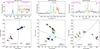 |
Fig. 1 Top: maser spectra of G37.43+1.51, G37.479–0.105, and G37.55+0.20 as obtained by EVN (color) and the Ibaraki radio telescope (gray line) on 24 October 2023. The vertical dashed lines indicate the system velocities. The horizontal magenta lines indicate velocity ranges of outflow indicators: CO for G37.43+1.51 (López-Sepulcre et al. 2010), the 44 GHz class I methanol maser (Cyganowski et al. 2009) for G37.479–0.105, and the SO 219.949 GHz line (Silva et al. 2017) for the G37.55+0.20. Bottom: distribution of methanol maser spots. The colors correspond to the LSR velocity as in the spectrum. The spot size is proportional to the logarithm of its brightness. The cloudlets (crosses) are numbered as listed in Tables A.1, B.1 and C.1. Additionally, we show the association of A or B groups to maser cloudlets for G37.43+1.51, as introduced in Surcis et al. (2015). The dashed lines show the PAs (direction axis) of the outflows. |
4.2 G37.479–0.105
One hundred fifty-three maser spots with velocities ranging from 53.6 to 63.4 km s−1 were detected from 14 cloudlets, which form two arc-like structures, within a region of ~100 mas×145 mas (1140 au×1650 au; Fig. 1, Table B.1). Comparing Ibaraki radio telescope and EVN spectra shows that only ~38% of the maser emission is resolved out.
Most cloudlets show an arched or complex distribution of spots with an internal gradient of velocity with respect to position. Cloudlets 1, 2, 4, 9, 10, and 11 have a double Gaussian profile, which is a high fraction (43%) of the total number of cloudlets. The angular extent of cloudlets ranges from 0.6 to 5.9 mas, with an average value of 2.1 mas, corresponding to Lproj = 23.1 ± 5.5 au. The velocity gradient ranges from 0.008 to 0.0695 km s−1 au−1 and the average value is 0.029 km s−1 au−1. The mean FWHM is 0.41 ± 0.03 km s−1. In a search for correlations between parameters, we found moderately strong correlations between FWHM and Lproj (r = 0.571, p < 0.001).
4.3 G37.55+0.20
The map of 139 maser spots forming 18 cloudlets in the LSR velocity range from 79.1 to 88.0 km s−1 is shown in Fig. 1 and listed in Table C.1. The emission is distributed over ~772 mas×255 mas corresponding to ~5147 au × 1500 au at a kinematic distance of 6.7 kpc (Fig. 1). Comparing Ibaraki single-dish spectra with the results from EVN shows that ~82% of the emission is resolved out.
All cloudlets have a single Gaussian profile, although a large portion (cloudlets 6, 1113, 14, and 17) have an incomplete profile for a good fit. The projected linear size of the cloudlets ranges from 0.4 to 8.0 mas, with an average value of 3.0 mas. The velocity gradient ranges from 0.06 to 0.84 km s−1 mas−1 with an average value of 0.23 km s−1 mas−1. The mean FWHM is 0.39 ± 0.03 km s−1. It is worth pointing out that overall, the detected masers are weaker compared to the other two sources, only three to five maser spots were detected in individual cloudlets, therefore making defined parameters comparably less accurate.
Flux densities from the Ibaraki monitoring campaign on 24 October 2023 (60 542 MJD) for the components show the flux as a function of time of the maser cloudlets (spectral features). At 79.62 km s−1 (cloudlet 5), the flux was at a minimum; at 83.77 km s−1 (superposition of cloudlets 1,2, and 3), it was in the dimming stage; the components at 84.55 and 84.92 km s−1 (the latter largely corresponds to cloudlet 7) were near maximum and began to dim; at 86.38 km s−1 (cloudlet 10), it was near its maximum; at 87.39 km s−1 (cloudlet 15), it was at a minimum; and at 87.82 km s−1 (cloudlet 16 and 18), it was in the dimming stage. The components at 85.63 an 85.84 km s−1 were too weak to reliably separate from other components and noise.
5 Analysis and discussion
5.1 G37.43+1.51
To estimate the relative proper motions in G37.43+1.51, the following procedure was applied: (1) cloudlets with positions and radial velocities consistent with those reported by Surcis et al. (2015) were identified; (2) the positional offsets relative to a chosen reference cloudlet were measured; and (3) linear motion was assumed over the 10.5 yr interval between the two epochs. The derived relative proper motions are shown in Fig. 2.
Most cloudlets exhibit PAs aligned within ~30° of their proper-motion vectors. In group A, all relative motion vectors are oriented along the linear distribution of the cloudlets. Clear symmetry is evident: cloudlets located east of the reference feature (cloudlet 5) move eastward, whereas those to the west move westward. This systematic behavior strongly suggests that the region traced by group A is undergoing expansion. The measured velocities for this group range from 0.7 to 1.8 km s−1, indicating relatively modest yet consistent outward motions.
Cloudlets belonging to group B, along with the isolated feature (cloudlet 7), display significantly higher relative velocities of 7.4 and 4.8 km s−1, respectively. Both appear to be moving away from group A.
The velocity range of group A is broadly consistent with that of the C18O outflow lobe (Surcis et al. 2015). However, our proper-motion results suggest that the 6.7 GHz methanol masers do not trace the outflow directly. Furthermore, despite the spectrum being dominated by the blueshifted masers, the velocity range of all masers (40.4–46.2 km s−1) centers on the systemic velocity of the region, indicating that the 6.7 GHz methanol maser emission has low relative velocity compared to the protostellar system itself. Since this species of masers is usually found within 103 au of the excitation energy source and given that the maser velocity is also near the region’s systemic velocity, we may expect the high-mass protostar to be located somewhere near the center of the overall distribution of the masers. The magnetic-field orientation in group A – previously shown to be perpendicular to the C18O outflow (López-Sepulcre et al. 2010; Surcis et al. 2015 and references therein) – forms an angle of about 25° with both the maser proper-motion vectors and their linear distribution. Taking all of the above into consideration, the 6.7 GHz methanol masers in this source may be associated with the upper layers of a circumstellar disk (Sanna et al. 2015). The 6.7 GHz CH3OH maser distribution in the YSO structure is consistent with a disk-wind model proposed for H2O and SiO masers (e.g., Moscadelli et al. 2019; Matthews et al. 2009). Alternatively, observed maser distribution and motion discrepancy with magnetic field direction could be explained with magnetically supported shocks, where the apparent deviation between magnetic-field orientation and maser velocity vectors or spatial distribution could be attributed to 3D projection effects, as proposed for H2O masers (e.g., Matthews et al. 2009).
We attempted to estimate the absolute proper motion of G37.43+1.51 masers by (1) measuring the phase-referenced coordinate differences between the two epochs, (2) dividing the resulting displacement by the time span between the EVN observations, and (3) subtracting the systematic motion of the source, as derived by Wu et al. (2014). Resulting proper motions correspond to several tens of kilometers per second, which is significantly higher than the typical ≲10 km s−1 expected for the 6.7 GHz maser. Such high velocities could result in the thermalization of the CH3OH molecule (Cragg et al. 2005). We conclude that the subtraction of the source’s systemic motion was not effective at isolating internal proper motions from absolute proper motions; therefore, a dedicated multi-epoch observing campaign should be initiated for this purpose.
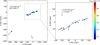 |
Fig. 2 Relative proper motion of the 6.7 GHz methanol maser cloudlets in G37.43+1.51. Right: Zoom-in on group A cloudlets with up-scaled motion vectors. |
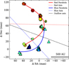 |
Fig. 3 Maser spot distribution in G37.479–0.105 with fitted parabolic structures and axes of symmetry. The triangles correspond to the maser spots associated with the blueshifted group, while the circles indicate the redshifted group. |
5.2 G37.479–0.105
The spatial distribution of the maser spots in G37.479–0.105 was analyzed to determine whether their arrangement follows parabolic structures (Fig. 3) often indicative of outflow cavity walls or bow shocks (Reid et al. 1988; Moscadelli & Cesaroni 2000). Using principal component analysis (PCA), the main orientation of each group of maser spots was established, and parabolic fits were applied in the rotated coordinate system. The corresponding axes of symmetry were derived from the fitted polynomials.
A statistical goodness-of-fit analysis based on the G-test (likelihood ratio test; Sokal & Rohlf 1995) was used to evaluate the validity of the parabolic fits. The redshifted maser group demonstrated excellent agreement with a parabolic distribution (G = 0.00, p = 1.00), which suggests an organized and coherent physical structure. In contrast, the blueshifted maser group produced a poor fit (G = 29.02, p < 0.001), showing larger deviations from the parabolic distribution. This could indicate distinct velocity components or simply reflect the sparseness of maser sampling in the structure – a common occurrence. The PAs of the symmetry axes of the parabolas traced by redshifted and blueshifted masers were 89° and 43°, respectively.
The 6.7 GHz methanol masers (which trace gas within 103 au of high-mass protostars) presented in this work are located at a central position between two sites of shock-tracing 44 GHz (Class I) methanol masers (Cyganowski et al. 2009). The tracer configuration suggests a central high-mass protostar symmetrically flanked by shock regions. The PA of the axis joining the shock tracers matches that of the symmetry axes of the parabolas described above. In the velocity domain, both maser species are also centered on the systemic velocity of the source. It is therefore highly likely that these two tracers form one protostar-outflow system where the 6.7 GHz maser parabolas delineate the base of an outflow cavity extending from the disk in the eastern direction, toward the region of blueshifted 44 GHz methanol masers. In this scenario, the G37.479–0.105 outflow would be oriented nearly in the plane of the sky, with the eastern lobe perhaps tilted slightly toward the observer. The apparent overlap of the blue- and redshifted 6.7 GHz methanol maser emission can be explained if the masers arise from opposite sides of the outflow cavity walls, with blueshifted cloudlets closer to us and the redshifted ones on the far side. The absence of 6.7 GHz maser emission along the opposite cavity is likely due to unfavorable conditions on the western side: masers are very sensitive to physical conditions, and a slight difference in, for example, density could quench the masers or significantly reduce their flux on the western side.
Future observations of cloudlet proper motions could test this hypothesis by searching for motion components along the outflow axis. Conversely, if the parabolas trace inflow streamers or spiral arms in the upper layers of a high-mass protostellar accretion disk, this hypothesis can also be tested by proper motion analyses.
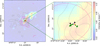 |
Fig. 4 Color map of G37.55+0.20 representing the SiO 86.846 GHz line, overlaid with the H2CO line at 89.188 GHz (grey contours, with the first level 15 times the 4.3 mJy beam−1 rms and steps equal to that value), and the C17O line at 336.6291 GHz (deep-pink contours, with the first level at 2.1 mJy beam−1 and 1.6 mJy beam−1 steps). All data were obtained from the ALMA archive. The maximum of the C-band continuum with JVLA is represented with an orange star (Araya et al. 2007). The H2CO maser emission at 4.83 GHz is represented with a magenta cross (Araya et al. 2005). The black triangles represent the positions of the 22 GHz water masers, as observed by JVLA (Beuther et al. 2002b). The Finlay 6.7 GHz methanol maser emission from this work is represented by green circles. |
5.3 G37.55+0.20
Comparing two EVN epochs reveals similar morphologies. In 2019, nine maser cloudlets were detected (compared to 18 in 2023), likely due to the lower signal-to-noise ratio (S/N). Of these, seven cloudlets closely match the velocities and relative positions of the features detected in 2023, while the remaining two may represent transient components located near other cloudlets.
A comparison with earlier 6.7 GHz methanol maser maps made using the Australian Telescope Compact Array (ATCA) by Beuther et al. (2002b) revealed that our contemporary EVN observations identified several additional maser cloudlets. While Beuther et al. (2002b) reported only three emission spots (see their Fig. 1), our maps show a substantially richer structure. Nevertheless, when the methanol maser distribution is overlaid with the positions of the H2CO and H2O masers reported in the literature (Araya et al. 2005; Beuther et al. 2002a), the relative spatial arrangement remains consistent: the methanol masers are located south of the water and formaldehyde masers (see Fig. 4). Of particular interest is cloudlet 5 (Vfit = 79.55 km s−1), which lies very near the reported position of the H2CO maser with a peak velocity of 79.5 km s−1. This positional and velocity coincidence makes it a good candidate for VLBA or EVN follow-up observations of both transitions to investigate potential coexistence.
To place the maser distribution in a broader physical context, we compare the 6.7 GHz methanol maser position obtained by EVN with additional molecular tracers observed with the Atacama Large Millimeter/submillimeter Array (ALMA). In Figure 4 we show additional molecular tracers extracted from ALMA archival data. The SiO 86.846 GHz transition, which traces outflow activity, is consistent with the results of Zhang et al. (2007). Meanwhile, the H2CO 89.188 GHz and C17O 336.6291 GHz lines – typically associated with protostellar disks – peak at positions close to that of the masers. Overall, the 22 GHz H2O, 4.83 GHz H2CO, and 6.7 GHz CH3OH masers, together with the peak of the C-band continuum emission, are clustered within ~100 mas (approximately 800 au). This compact configuration is consistent with the peak positions of the SiO, H2CO, and C17O lines observed with ALMA. Since the 6.7 GHz methanol masers are proximal to both the spatial center and velocity center of the system, it is therefore apparent that the 6.7 GHz methanol masers trace the inner-most regions of the protostellar system from where the aforementioned outflows are launched.
While the spatial distribution constrains the geometry of the system, long-term variability could provide independent information on its 3D structure and possible powering mechanisms. The G37.55+0.20 6.7 GHz methanol masers were monitored with the Irbene radio telescopes, revealing interesting variability patterns (Aberfelds et al. 2023b). Notably, the spectral component near 83.8 km s−1 (arising from the superposition of cloudlets 1, 2, and 3) reaches its maximum intensity approximately one month earlier than the 84.8 km s−1 component (cloudlet 7), located at a projected separation of ~190 mas (1280 au) from the former group. If variability were driven solely by additional seed photons from the continuum source, this order of variability would be plausible. However, the observed time delay is inconsistent with light-travel times: the projected separation of 1280 au corresponds to a delay much shorter than the ~5200 au required to explain the observed lag. A possible explanation is that the cloudlet groups are significantly separated along the line of sight, with cloudlets 1–3 located much closer to the observer than cloudlet 7. Such a 3D structure would reconcile the observed variability sequence and delay. Alternatively, changes in the physical conditions of the maser emission region propagating at a sub-luminal speed (~0.25c) could explain the component time delays, similar to the case of G24.33+0.14 (Kobak et al. 2023). However, in this scenario the projected distance would fully represent the physical separation between cloudlets 1, 2, 3, and 7. Furthermore, the relatively bright (0.67 mJy) continuum source detected toward G37.55+0.20 by Hu et al. (2016) makes this region a promising candidate in which the colliding-wind binary model could potentially account for the observed maser variability.
Since the period of the potential colliding-wind binary – traced by 6.7 GHz methanol maser variability – is known, sensitive continuum monitoring observations could validate the colliding-wind binary hypothesis. In addition, a VLBI maser imaging monitoring campaign could determine whether the timing differences in maser flux variations across different velocity features are due to seed photon variability, light travel times of pumping radiation, or the sub-luminal propagation of maser pumping conditions. This would be based on a more precise evaluation of the spacial locations of each spectral component.
6 Conclusions
We obtained and analyzed milliarcsecond resolution images for three 6.7 GHz methanol maser sources associated with HMYSOs. Two of these (G37.479–0.105 and G37.55+0.20) were imaged at this frequency and resolution for the first time. We conclude the following:
(i) The 6.7 GHz methanol masers in G37.43+1.51 appear largely unchanged since earlier observations in 2013, indicating no drastic changes in the physical or radiative properties of the central region of the high-mass protostellar system during this period. The relative proper motion vectors in G37.43+1.51 are along the major cloudlet distribution axes. The brightest and longest distribution of methanol masers expands at a speed of about 1.1 km s−1. Although the northern group (group A) of 6.7 GHz methanol masers has the same velocity range as the blueshifted lobe of the C18O outflow, our results suggest that maser cloudlets do not follow this outflow-bound motion.
(ii) The redshifted maser cloudlets in G37.479–0.105 from a well-defined parabolic structure with an excellent fit, whereas the blueshifted cloudlets are somewhat more scattered around an overall parabolic shape. The symmetric axes of these parabolas match the PAs of the two sites of the Class I methanol masers reported in the literature, indicating that the 6.7 GHz methanol masers sit at the center of a high-mass protostar driving a bipolar outflow. The overall distribution of maser cloudlets indicate that they may trace the wall of outflow cavity.
(iii) In G37.55+0.20, the time delays in spectral component variability, considering the locations of the corresponding maser cloudlets, suggest that the two main spectral components (83.8 and 84.8 km s−1) are separated by at least 5200 au (assuming the maser pumping conditions are modulated at the speed of light). This is significantly more than their projected separation (1300 au), which could mean they trace gas on opposite sides of the YSO. Overall, variability seen in G37.55+0.20 could be explained with a colliding-wind binary model.
Data availability
EVN data are available at http://archive.jive.nl. The single-dish data are available at https://vlbi.sci.ibaraki.ac.jp/iMet. (Yonekura et al. 2016). The ALMA data are publicly available at https://almascience.nao.ac.jp/aq/ (project id: 2015.1.00369.S).
Acknowledgements
We thank the referee for their comments and suggestions, which improved the manuscript. This publication has received funding from the Latvian Council of Science project “A single–baseline radio interferometer in a new age of transient astrophysics (IVARS)” (lzp-2022/1-0083). The European VLBI Network is a joint facility of independent European, African, Asian, and North American radio astronomy institutes. Scientific results from data presented in this publication are derived from the following EVN project code: EA072 This work made use of Astropy4: a community–developed core Python package and an ecosystem of tools and resources for astronomy (Astropy Collaboration 2013, 2018, 2022), matplotlib (Hunter 2007), and numpy and scipy (Virtanen et al. 2020).
References
- Aberfelds, A., Bartkiewicz, A., Szymczak, M., et al. 2023a, MNRAS, 524, 599 [Google Scholar]
- Aberfelds, A., Šteinbergs, J., Shmeld, I., & Burns, R. A. 2023b, MNRAS, 526, 5699 [Google Scholar]
- Al-Marzouk, A. A., Araya, E. D., Hofner, P., et al. 2012, ApJ, 750, 170 [Google Scholar]
- Araya, E., Hofner, P., Kurtz, S., et al. 2005, ApJ, 618, 339 [Google Scholar]
- Araya, E., Hofner, P., Sewiło, M., et al. 2007, ApJ, 669, 1050 [Google Scholar]
- Araya, E. D., Hofner, P., Goss, W. M., et al. 2010, ApJ, 717, L133 [Google Scholar]
- Astropy Collaboration (Robitaille, T. P., et al.) 2013, A&A, 558, A33 [NASA ADS] [CrossRef] [EDP Sciences] [Google Scholar]
- Astropy Collaboration (Price-Whelan, A. M., et al.) 2018, AJ, 156, 123 [Google Scholar]
- Astropy Collaboration (Price-Whelan, A. M., et al.) 2022, ApJ, 935, 167 [NASA ADS] [CrossRef] [Google Scholar]
- Bartkiewicz, A., Szymczak, M., & van Langevelde, H. J. 2005, A&A, 442, L61 [NASA ADS] [CrossRef] [EDP Sciences] [Google Scholar]
- Bartkiewicz, A., Szymczak, M., van Langevelde, H. J., Richards, A. M. S., & Pihlström, Y. M. 2009, A&A, 502, 155 [NASA ADS] [CrossRef] [EDP Sciences] [Google Scholar]
- Bartkiewicz, A., Szymczak, M., & van Langevelde, H. J. 2014, A&A, 564, A110 [NASA ADS] [CrossRef] [EDP Sciences] [Google Scholar]
- Bartkiewicz, A., Szymczak, M., & van Langevelde, H. J. 2016, A&A, 587, A104 [NASA ADS] [CrossRef] [EDP Sciences] [Google Scholar]
- Bartkiewicz, A., Sanna, A., Szymczak, M., et al. 2020, A&A, 637, A15 [NASA ADS] [CrossRef] [EDP Sciences] [Google Scholar]
- Beuther, H., Schilke, P., Sridharan, T. K., et al. 2002a, A&A, 383, 892 [NASA ADS] [CrossRef] [EDP Sciences] [Google Scholar]
- Beuther, H., Walsh, A., Schilke, P., et al. 2002b, A&A, 390, 289 [NASA ADS] [CrossRef] [EDP Sciences] [Google Scholar]
- Beuther, H., Kuiper, R., & Tafalla, M. 2025, ARA&A, 63, 1 [Google Scholar]
- Chabrier, G. 2003, PASP, 115, 763 [Google Scholar]
- Cragg, D. M., Sobolev, A. M., & Godfrey, P. D. 2005, MNRAS, 360, 533 [Google Scholar]
- Cyganowski, C. J., Whitney, B. A., Holden, E., et al. 2008, AJ, 136, 2391 [Google Scholar]
- Cyganowski, C. J., Brogan, C. L., Hunter, T. R., & Churchwell, E. 2009, ApJ, 702, 1615 [NASA ADS] [CrossRef] [Google Scholar]
- Dodson, R., Ojha, R., & Ellingsen, S. P. 2004, MNRAS, 351, 779 [NASA ADS] [CrossRef] [Google Scholar]
- Fujisawa, K., Sugiyama, K., Motogi, K., et al. 2014, PASJ, 66, 31 [NASA ADS] [Google Scholar]
- Goddi, C., Moscadelli, L., & Sanna, A. 2011, A&A, 535, L8 [NASA ADS] [CrossRef] [EDP Sciences] [Google Scholar]
- Goedhart, S., Gaylard, M. J., & van der Walt, D. J. 2004, MNRAS, 355, 553 [Google Scholar]
- Greif, T. H. 2015, Computat. Astrophys. Cosmol., 2, 3 [Google Scholar]
- Hu, B., Menten, K. M., Wu, Y., et al. 2016, ApJ, 833, 18 [Google Scholar]
- Hunter, J. D. 2007, Comput. Sci. Eng., 9, 90 [NASA ADS] [CrossRef] [Google Scholar]
- Inayoshi, K., Sugiyama, K., Hosokawa, T., et al. 2013, ApJ, 769, L20 [NASA ADS] [CrossRef] [Google Scholar]
- Keimpema, A., Kettenis, M., Pogrebenko, S., et al. 2015, Exp. Astron., 39, 259 [NASA ADS] [CrossRef] [Google Scholar]
- Kobak, A., Bartkiewicz, A., Szymczak, M., et al. 2023, A&A, 671, A135 [NASA ADS] [CrossRef] [EDP Sciences] [Google Scholar]
- López-Sepulcre, A., Cesaroni, R., & Walmsley, C. M. 2010, A&A, 517, A66 [NASA ADS] [CrossRef] [EDP Sciences] [Google Scholar]
- Matthews, L. D., Greenhill, L. J., Goddi, C., et al. 2009, ApJ, 708, 80 [Google Scholar]
- Menten, K. M. 1991, ApJ, 380, L75 [Google Scholar]
- Moscadelli, L., & Cesaroni, R. 2000, A&A, 361, L33 [Google Scholar]
- Moscadelli, L., & Goddi, C. 2014, A&A, 566, A150 [NASA ADS] [CrossRef] [EDP Sciences] [Google Scholar]
- Moscadelli, L., Cesaroni, R., Rioja, M. J., Dodson, R., & Reid, M. J. 2011a, A&A, 526, A66 [NASA ADS] [CrossRef] [EDP Sciences] [Google Scholar]
- Moscadelli, L., Sanna, A., & Goddi, C. 2011b, A&A, 536, A38 [NASA ADS] [CrossRef] [EDP Sciences] [Google Scholar]
- Moscadelli, L., Sanna, A., Goddi, C., et al. 2019, A&A, 631, A74 [NASA ADS] [CrossRef] [EDP Sciences] [Google Scholar]
- Pandian, J. D., Momjian, E., Xu, Y., Menten, K. M., & Goldsmith, P. F. 2011, ApJ, 730, 55 [NASA ADS] [CrossRef] [Google Scholar]
- Parfenov, S. Y., & Sobolev, A. M. 2014, MNRAS, 444, 620 [Google Scholar]
- Reid, M. J., Schneps, M. H., Moran, J. M., et al. 1988, ApJ, 330, 809 [Google Scholar]
- Reid, M. J., Menten, K. M., Brunthaler, A., et al. 2019, ApJ, 885, 131 [Google Scholar]
- Rygl, K. L. J., Brunthaler, A., Reid, M. J., et al. 2010, A&A, 511, A2 [NASA ADS] [CrossRef] [EDP Sciences] [Google Scholar]
- Sanna, A., Moscadelli, L., Cesaroni, R., et al. 2010a, A&A, 517, A71 [NASA ADS] [CrossRef] [EDP Sciences] [Google Scholar]
- Sanna, A., Moscadelli, L., Cesaroni, R., et al. 2010b, A&A, 517, A78 [NASA ADS] [CrossRef] [EDP Sciences] [Google Scholar]
- Sanna, A., Surcis, G., Moscadelli, L., et al. 2015, A&A, 583, L3 [NASA ADS] [CrossRef] [EDP Sciences] [Google Scholar]
- Sanna, A., Moscadelli, L., Surcis, G., et al. 2017, A&A, 603, A94 [NASA ADS] [CrossRef] [EDP Sciences] [Google Scholar]
- Silva, A., Zhang, Q., Sanhueza, P., et al. 2017, ApJ, 847, 87 [Google Scholar]
- Sokal, R. R., & Rohlf, F. J. 1995, Biometry: The Principles and Practice of Statistics in Biological Research, 3rd edn. (W. H. Freeman) [Google Scholar]
- Sridharan, T. K., Beuther, H., Schilke, P., Menten, K. M., & Wyrowski, F. 2002, ApJ, 566, 931 [Google Scholar]
- Sugiyama, K., Fujisawa, K., Doi, A., et al. 2014, A&A, 562, A82 [NASA ADS] [CrossRef] [EDP Sciences] [Google Scholar]
- Surcis, G., Vlemmings, W. H. T., van Langevelde, H. J., et al. 2015, A&A, 578, A102 [NASA ADS] [CrossRef] [EDP Sciences] [Google Scholar]
- Szymczak, M., Wolak, P., & Bartkiewicz, A. 2014, MNRAS, 439, 407 [NASA ADS] [CrossRef] [Google Scholar]
- Szymczak, M., Wolak, P., & Bartkiewicz, A. 2015, MNRAS, 448, 2284 [NASA ADS] [CrossRef] [Google Scholar]
- Szymczak, M., Olech, M., Sarniak, R., Wolak, P., & Bartkiewicz, A. 2017, MNRAS, 474, 219 [Google Scholar]
- van der Walt, D. J. 2011, ApJ, 141, 152 [Google Scholar]
- van der Walt, D. J. 2014, A&A, 562, A68 [NASA ADS] [CrossRef] [EDP Sciences] [Google Scholar]
- Van Der Walt, D. J., Goedhart, S., & Gaylard, M. J. 2009, MNRAS, 398, 961 [NASA ADS] [CrossRef] [Google Scholar]
- Virtanen, P., Gommers, R., Oliphant, T. E., et al. 2020, Nat. Med., 17, 261 [Google Scholar]
- Wu, Y. W., Sato, M., Reid, M. J., et al. 2014, A&A, 566, A17 [NASA ADS] [CrossRef] [EDP Sciences] [Google Scholar]
- Wu, Y. W., Reid, M. J., Sakai, N., et al. 2019, ApJ, 874, 94 [NASA ADS] [CrossRef] [Google Scholar]
- Yonekura, Y., Saito, Y., Sugiyama, K., et al. 2016, PASJ, 68, 74 [NASA ADS] [CrossRef] [Google Scholar]
- Zhang, Q., Sridharan, T. K., Hunter, T. R., et al. 2007, A&A, 470, 269 [NASA ADS] [CrossRef] [EDP Sciences] [Google Scholar]
- Zinnecker, H., & Yorke, H. W. 2007, ARA&A, 45, 481 [Google Scholar]
Appendix A Parameters of the 6.7 GHz methanol maser cloudlets in G37.43+1.51
Parameters of the 6.7 GHz methanol maser cloudlets in G37.43+1.51.
Appendix B Parameters of the 6.7 GHz methanol maser cloudlets in G37.479–0.105
Parameters of the 6.7 GHz methanol maser cloudlets in G37.479–0.105.
Appendix C Parameters of the 6.7 GHz methanol maser cloudlets in G37.55+0.20
Parameters of the 6.7 GHz methanol maser cloudlets in G37.55+0.20.
All Tables
All Figures
|
Fig. 1 Top: maser spectra of G37.43+1.51, G37.479–0.105, and G37.55+0.20 as obtained by EVN (color) and the Ibaraki radio telescope (gray line) on 24 October 2023. The vertical dashed lines indicate the system velocities. The horizontal magenta lines indicate velocity ranges of outflow indicators: CO for G37.43+1.51 (López-Sepulcre et al. 2010), the 44 GHz class I methanol maser (Cyganowski et al. 2009) for G37.479–0.105, and the SO 219.949 GHz line (Silva et al. 2017) for the G37.55+0.20. Bottom: distribution of methanol maser spots. The colors correspond to the LSR velocity as in the spectrum. The spot size is proportional to the logarithm of its brightness. The cloudlets (crosses) are numbered as listed in Tables A.1, B.1 and C.1. Additionally, we show the association of A or B groups to maser cloudlets for G37.43+1.51, as introduced in Surcis et al. (2015). The dashed lines show the PAs (direction axis) of the outflows. |
| In the text | |
|
Fig. 2 Relative proper motion of the 6.7 GHz methanol maser cloudlets in G37.43+1.51. Right: Zoom-in on group A cloudlets with up-scaled motion vectors. |
| In the text | |
|
Fig. 3 Maser spot distribution in G37.479–0.105 with fitted parabolic structures and axes of symmetry. The triangles correspond to the maser spots associated with the blueshifted group, while the circles indicate the redshifted group. |
| In the text | |
|
Fig. 4 Color map of G37.55+0.20 representing the SiO 86.846 GHz line, overlaid with the H2CO line at 89.188 GHz (grey contours, with the first level 15 times the 4.3 mJy beam−1 rms and steps equal to that value), and the C17O line at 336.6291 GHz (deep-pink contours, with the first level at 2.1 mJy beam−1 and 1.6 mJy beam−1 steps). All data were obtained from the ALMA archive. The maximum of the C-band continuum with JVLA is represented with an orange star (Araya et al. 2007). The H2CO maser emission at 4.83 GHz is represented with a magenta cross (Araya et al. 2005). The black triangles represent the positions of the 22 GHz water masers, as observed by JVLA (Beuther et al. 2002b). The Finlay 6.7 GHz methanol maser emission from this work is represented by green circles. |
| In the text | |
Current usage metrics show cumulative count of Article Views (full-text article views including HTML views, PDF and ePub downloads, according to the available data) and Abstracts Views on Vision4Press platform.
Data correspond to usage on the plateform after 2015. The current usage metrics is available 48-96 hours after online publication and is updated daily on week days.
Initial download of the metrics may take a while.