| Issue |
A&A
Volume 708, April 2026
|
|
|---|---|---|
| Article Number | A170 | |
| Number of page(s) | 13 | |
| Section | The Sun and the Heliosphere | |
| DOI | https://doi.org/10.1051/0004-6361/202658932 | |
| Published online | 03 April 2026 | |
Neural blind deconvolution to reconstruct high-resolution ground-based solar observations
1
Institute of Physics, University of Graz, Universitätsplatz 5, 8010 Graz, Austria
2
High Altitude Observatory, NSF National Center for Atmospheric Research, 3080 Center Green Dr, Boulder, USA
3
Kanzelhöhe Observatory for Solar and Environmental Research, University of Graz, Treffen am Ossiacher See, Austria
4
National Solar Observatory, 3665 Discovery Drive, Boulder, CO 80303, USA
★ Corresponding author: This email address is being protected from spambots. You need JavaScript enabled to view it.
Received:
12
January
2026
Accepted:
3
March
2026
Abstract
Context. Ground-based solar observations enable unprecedented spatial, spectral, and temporal resolution of the lower solar atmosphere, yet Earth’s turbulent atmosphere imposes significant limitations, requiring advanced post facto image reconstruction. State-of-the-art reconstruction methods are based on restoring a burst of short exposure frames to a single observation. Limitations of these techniques arise due to the sparse information available concerning the atmospheric point spread function (PSF), which degrades the observations and, consequently, the quality of reconstructions. Developing new reconstruction methods is essential for providing high-quality data products for the study of the lower solar atmosphere on the smallest scales.
Aims. We aim to develop a novel image-reconstruction method to achieve unprecedented spatial resolution from short exposure image bursts. This can provide high-quality reconstructions and therefore advance the study of the smallest spatial scales from the solar photosphere to the chromosphere.
Methods. In this paper, we present a novel approach for high-resolution solar-image reconstruction based on physics-informed neural networks. In the training process, the neural network maps coordinate points (x, y) directly to their corresponding intensity values o(x, y), while simultaneously updating the PSF parameters. The method convolves the "true" object from the neural network with the estimated PSFs and optimizes the network by minimizing the loss between the synthesized and real short-exposure image burst. This approach enabled the simultaneous estimation of both the degrading PSF and the real high-resolution intensity distribution.
Results. We demonstrate the method on synthetic intensity data derived from a radiative magnetohydrodynamics (MHD) simulation, where we applied PSF convolution and noise to obtain a realistic synthetic input data set, similar to observational short-exposure observations. Quantitative comparisons using image quality metrics, histograms, and power spectral analysis confirm that the model can reliably reconstruct the original image from the stack of synthetic short-exposure frames. Finally, we applied our method to high-resolution observations from GREGOR and DKIST and compare to state-of-the-art speckle reconstructions and multi-frame blind deconvolutions. Our results demonstrate the ability to reconstruct small-scale solar features that exceed the reconstruction performance of state-of-the-art reconstruction methods. With this approach, we lay the foundation for future spatially varying PSFs.
Key words: atmospheric effects / techniques: image processing / telescopes / Sun: atmosphere / Sun: chromosphere / Sun: photosphere
© The Authors 2026
 Open Access article, published by EDP Sciences, under the terms of the Creative Commons Attribution License (https://creativecommons.org/licenses/by/4.0), which permits unrestricted use, distribution, and reproduction in any medium, provided the original work is properly cited.
This article is published in open access under the Subscribe to Open model. This email address is being protected from spambots. You need JavaScript enabled to view it. to support open access publication.
1. Introduction
Large-aperture solar telescopes provide high-resolution observations, enabling detailed studies on very small scales in the different atmospheric layers of the Sun, from the solar photosphere to the lower solar corona. Such high-quality observations are essential for studying the Sun’s dynamic processes and magnetic activity. Turbulent plasma motions within the convection zone and strong magnetic fields are key drivers of energetic eruptive phenomena, including solar flares and coronal mass ejections (Priest & Forbes 2002; Wiegelmann et al. 2014). However, observations from large-aperture ground-based telescopes are affected by Earth’s turbulent atmosphere. While the wavefront from a distant point source can be considered as flat outside Earth’s atmosphere, atmospheric turbulence introduces phase errors that lead to image degradation and blurring in the observational data (McKechnie 1992; Quirrenbach 2006). State-of-the-art high-resolution telescopes are equipped with adaptive optics (AO) systems, which aim to minimize the phase errors in the wavefront and thus reduce the distortion in the observations (Rimmele & Marino 2011). Nevertheless, due to turbulence in multiple layers of the Earth’s atmosphere, these corrections are challenging, which limits the spatial and spectral resolution of the observations (Rimmele et al. 2008). Equipped with four-meter mirrors, the Daniel K. Inouye Solar Telescope (DKIST; Rimmele et al. 2020) and the future European Solar Telescope (EST; Quintero Noda et al. 2022) offer unprecedented spatial, spectral, and temporal resolution for studying the solar atmosphere. However, they also require sophisticated image reconstruction methods to achieve their full resolution potential. Post facto image reconstructions provide the only option to account for the remaining atmospheric degradations and to achieve the diffraction-limited resolution of large-aperture telescopes. (Löfdahl et al. 2002).
State-of-the-art reconstruction methods such as speckle reconstruction, multi-frame blind deconvolution (MFBD) and multi-object multi-frame blind deconvolution (MOMFBD) are based on the assumption that the real object is distorted by the convolution with an unknown point spread function (PSF) and an additional noise term (Knox & Thompson 1974; de Boer & Kneer 1992; Löfdahl & Scharmer 2003; Schulz 1993; Van Noort et al. 2005). Short exposure observations preserve information in the higher frequency domain, quasi “freezing” the state of the turbulent atmosphere, to retain the diffraction-limited information (Labeyrie 1970). For a high-cadence image burst it can be assumed that the solar features remain unchanged, while the atmospheric degradations change on a much shorter timescale. Consequently, using a burst of short exposure observations improves the quality of the reconstruction (Wöger et al. 2008). The image formation of the burst can be described as the convolution of the real object o(r) with the PSFs pk(r) and the addition of a noise terms nk(r), which is primarily attributed to photon noise:
 (1)
(1)
where r = (x, y) are the coordinates in the image space and k indexes individual image frames, k = 1…K, with K representing the total number of frames in a burst. The PSFs are composed of the telescope PSF and the PSFs from the turbulent atmosphere.
For MFBD and MOMFBD, this problem is ill-posed for a single image, since neither the real object nor the PSFs of the turbulent atmosphere are known for the deconvolution process. In order to solve this problem to estimate o(r), a stack of short-exposure images is used and is described by Van Noort et al. (2005). Here, the image formation (Eq. 1) is expressed in the Fourier domain as
 (2)
(2)
where Pk(u) is the optical transfer function (OTF), i.e., the Fourier transform of the PSF. In MFBD, the PSF is initialized through a wavefront in the pupil plane. The phase is constructed with a finite set of of basis functions, Bm(ξ), and wavefront coefficients, αk, m, following
 (3)
(3)
Using this phase representation, the OTF can be written as
![Mathematical equation: $$ \begin{aligned} P_k(u) = \mathcal{F} \left\{ \left| \mathcal{F} ^{-1} \left[A(\xi ) \,\exp \!\left( i \, \varphi _k(\xi ) \right)\right] \right|^2 \right\} , \end{aligned} $$](/articles/aa/full_html/2026/04/aa58932-26/aa58932-26-eq4.gif) (4)
(4)
with A(ξ) corresponding to the pupil function. Finally, solving Eq. (2) corresponds to a joint least-squares optimization over the object and the wavefront coefficients:
 (5)
(5)
where  and
and  correspond to estimated quantities. Under the assumption of additive Gaussian noise, the estimation of true object intensities,
  , can be written as
 (6)
(6)
reducing the least-squares optimization to the  only. Here, * denotes complex conjugations, and H(u) corresponds to a low-pass filter from Löfdahl & Scharmer (1994), for example.
In contrast to MFBD and MOMFBD, speckle reconstruction follows a statistical approach in which the Fourier amplitudes and phases are estimated separately. The Fourier phases are recovered using a generalization of the Knox–Thompson method, the speckle masking technique, which evaluates the bispectrum (triple correlations in Fourier space) to obtain robust phase estimates of the true object (Lohmann et al. 1983). The Fourier amplitudes are determined following the method of Labeyrie (1970), which requires knowledge of the speckle transfer function (STF). To determine the STF, the spectral ratio is computed and compared with atmospheric turbulence models to estimate the Fried parameter (r0), which is a measure of the strength of the atmospheric seeing (von der Luehe 1984). Once the STF is known, the true object’s spatial power spectrum can be reconstructed, and together with the recovered phases an estimate of the true object intensity distribution can be obtained (Wöger et al. 2008).
Limitations of state-of-the-art methods can arise from reconstruction artifacts as well as their high computational cost. The methods work under isoplanatic conditions (non-field-dependent PSF), meaning that the wavefront distortions are constant across the image. Consequently, only small patches can be reconstructed, which limits the effectiveness when a large field of view (FOV) needs to be restored. Mosaicing these patches can enable large FOV reconstructions, but it can also introduce artifacts in the restorations. Furthermore, the reconstruction methods currently in use are based in the Fourier domain. Transforming back and forth between the Fourier and image domain can introduce artifacts, which may further degrade the reconstruction quality. Additionally, estimating the true PSF is challenging. MFBD makes assumptions using a set of basis functions and wavefront coefficients to estimate the PSF, which can make it difficult to fully recover the true PSF. Errors in PSF estimation propagate into the reconstructed image, causing artifacts or loss of resolution (Löfdahl & Scharmer 1994; Van Noort et al. 2005; Löfdahl et al. 2006).
To overcome these limitations, Asensio Ramos et al. (2018) first applied convolutional neural networks to reconstruct a burst of degraded observations. In a follow-up paper, Asensio Ramos et al. (2023) used deep neural networks to accelerate the deconvolution problem, employing the same approach as the MOMFBD method. This involves using a set of basis functions to simultaneously estimate the PSF and the real object. Following the MOMFBD methodology, Asensio Ramos (2024) employed a neural emulator network with a spatially variant PSF to mitigate the effects of anisoplanatism. Schirninger et al. (2025) applied generative adversarial networks (GANs; Goodfellow et al. 2020) to reconstruct a burst of observation to a single high-quality, high-resolution observation.
The proposed NeuralBD method is a new reconstruction method where we solve the image equation given in Eq. (1). The method is based on physics-informed neural networks (PINNs; Raissi et al. 2019; Karniadakis et al. 2021), which have already been shown to successfully incorporate physical models with noisy observational data in solar physics (Jarolim et al. 2023, 2024; Díaz Baso et al. 2025; Jarolim et al. 2025). Our NeuralBD model uses a neural network to encode input coordinates (x, y) to pixel intensity values o(x, y). The training process involves estimating the PSF, computing the convolution in the image domain, and minimizing the residuals between the estimated and original burst of observation. Using a PINN enables a smooth representation of the image while requiring relatively low memory, as no training dataset is needed. Instead, the image equation (Eq. 1) is solved iteratively, allowing simultaneous estimation of both the PSFs and the true intensity distribution of the object. This represents a novel approach compared to state-of-the-art reconstruction methods, as the problem is solved directly in the image domain rather than in the Fourier domain. This lays the foundations to extending this method to spatially varying PSFs allowing reconstruction over a larger FOV.
In this study, we present an image-reconstruction method based on the simultaneous estimation of the distorting PSF and the real object. In our approach, the PSF does not consider any constraints except pixel size, by iteratively updating the PSF parameters in the training step. NeuralBD is a solver-based method rather than a function approximator such as classical deep-learning models. Consequently, it is more computationally expensive, but provides solutions independent of any reference data set. This makes the approach applicable to any high-resolution broadband imaging instrument and offers the possibility to find more effective solutions of the PSF and therefore, the real object reconstruction. We demonstrate that our NeuralBD method can estimate the real object and the PSF simultaneously. To test the model and to quantify its performance, we applied it to simulation data and real observations.
2. Method
The aim of our NeuralBD method is to estimate the real object intensity distribution by solving the inverse problem as described in Eq. (1). The neural network serves as a smooth function approximation of the real object, o(x, y), where the coordinate points (x, y) are mapped to intensity values o(x, y). By iteratively updating the real object and the PSFs, we calculated the convolution to match the observed image burst, ik(x, y). This is contrary to MFBD, which performs the least-squares optimization in the Fourier domain (Eq. 5) and only depends on the estimation of the OTFs.
We approximated the continuous object-intensity distribution by learning a mapping (x, y)↦o(x, y). Our pixel coordinates are first centered around zero and then normalized by dividing by 1024. We sampled the normalized coordinate points and applied a random perturbation within each grid cell, rather than only evaluating the network at pixel centers. This perturbed sampling avoids restricting the model to fixed pixel centers and instead enables the network to represent a continuous intensity distribution, which corresponds to a stochastic sub-pixel sampling of the underlying image domain.
The second step in our NeuralBD pipeline is to estimate the true PSFs for the deconvolution process. In contrast to conventional approaches of constraining the PSFs with a set of basis functions and wavefront coefficients, we fully modeled the PSF as a set of N × N pixel free parameters from an arbitrary distribution. The initialization of the PSFs was performed using a centered normal distribution with a mean of zero and a standard deviation of five pixels (μ = 0, σ = 5). However, the initialization can be chosen arbitrarily, for example by sampling from a random distribution or also using the Karhunen–Loéve polynomials with the wavefront coefficients. For the deconvolution process, the number of PSFs corresponds to the number of frames in the burst (n). The only constraint we set for the PSF is that each PSF must sum to one and must be positive, following
 (7)
(7)
Based on the selected number of frames, we generated K corresponding PSFs to perform the convolution. The 2D PSF parameters were optimized by initializing them as learnable parameters within the model and scale them, where the output of the PSFs corresponds to exp(log_PSFk), where k corresponds to the index of the PSF.
Third, we calculated the convolution of the estimated object-intensity distribution o(x, y) using the estimated PSFs in the image space. We approximated the continuous convolution,
 (8)
(8)
by a discrete quadrature over the perturbed sampling locations,
 (9)
(9)
where  denotes the estimated short-exposure image burst,
  the true object-intensity distribution, and
  the corresponding PSFs estimated by the NeuralBD model. The term a(x′,y′) indicates the local area elements associated with each perturbed sampling point and corresponds to the quadrature weights approximating the differential surface element dA = dξ dη. These weights were computed from the distances between adjacent perturbed sampling locations and ensure conservation of PSF unity in the discretized convolution. After calculating the convolution, we employed a mean squared error (MSE) loss computed between the synthesized burst and the original burst of observation for the optimization of the neural network and the PSF parameters. The optimization is carried out through an iterative process during which both the real object intensity distribution and the PSF parameters are progressively updated.
The NeuralBD image model was implemented as a fully connected neural network consisting of eight hidden layers with 512 neurons each. We utilized a sine activation function on each layer, inspired by the sinusoidal representation networks (SIREN; Sitzmann et al. 2020). Before we fed the coordinate points into the first layer, we employed a Gaussian positional encoding. Consequently, we encoded the input coordinates into Fourier features of sin and cos functions. Here, we chose 128 random frequencies from a normal distribution scaled between zero and four (fi ∼ 𝒩(0, 4)), which we found to give the best results. The resulting encoding is given by
![Mathematical equation: $$ \begin{aligned} \begin{aligned} \nu _{\text{encoded}} = [\sin (f_{x,0}\cdot x), \cos (f_{x,0}\cdot x), \sin (f_{x,1}\cdot x), \\ \cos (f_{x,1}\cdot x),\,\ldots \,, \sin (f_{y,127}\cdot y), \cos (f_{y,127}\cdot y)], \end{aligned} \end{aligned} $$](/articles/aa/full_html/2026/04/aa58932-26/aa58932-26-eq17.gif) (10)
(10)
with fi, j corresponding to the jth sampled frequency of coordinate, i. Incorporating Gaussian positional encoding allows for better selection of high-frequency terms producing sharper reconstructions, while the comparison with a classical SIREN network resulted in less sharp reconstruction and slower convergence. The frequencies of the encoding are decisive for the success of the method, as it controls the ability to encode high-frequency features (Tancik et al. 2020). Frequencies that are too high may introduce artifacts in the reconstruction, whereas frequencies that are too low fail to capture fine structural details. Additionally, the Fourier feature regularization acts as implicit noise damping due to the model’s bias toward lower frequency representations. Consequently, NeuralBD does not require a noise filter. The input layer then takes the encoded coordinate points and the neural network maps them to the intensity values o(x, y). For output activation, we found that an exponential function with base 10 gives the best results. To accelerate the reconstruction process, we first pre-trained the image model o(x, y) for 300 epochs using the original frame with the lowest root-mean-square (RMS) error as reference. This initialization allows the model to start from a reasonable estimate of the object, rather than learning the image from scratch, and consequently it can focus directly on the reconstruction task. Note that in principle reconstruction from scratch is also possible, but the reconstruction time would be significantly increased, while performance is comparable.
To validate the performance of our NeuralBD method, we considered three image reconstruction methods for comparison: a classical deconvolution technique, a reconstruction method based on a state-of-the-art technique, and a state-of-the-art reconstruction method commonly used for high-resolution solar observations. In this study, the Richardson–Lucy deconvolution served as the baseline reconstruction method (Richardson 1972). We applied the Richardson–Lucy deconvolution to the simulation data, where we used the known ground-truth PSFs as input for the reconstruction. The number of iterations was set to 1000, which we found to provide the best results empirically in terms of sharpness and stability. A lower number of iterations leads to reconstructions that are less sharp. As a second comparison, we employed a multi-frame blind deconvolution approach using the torchmfbd method of Asensio Ramos et al. (2025). We used the default implementation while adapting the configuration parameters to match the observational setup of the different instruments. This method is used for the comparison of both the simulation data and the high-resolution observations obtained from GREGOR and DKIST. In addition, we used speckle reconstructions for the comparison of high-resolution observational data. For GREGOR, the speckle reconstructions were obtained using the KISIP software package from Wöger & von der Lühe (2008), while for DKIST they were carried out using the method described in Beard et al. (2020). To evaluate the power spectral density (PSD) of each observation including the convolved frames from the simulation data, the original frames from the real observations, the NeuralBD reconstructions, and the high-quality reference observations, we used and adapted the azimuthal PSD implementation from Asensio Ramos (2024). The PSD was calculated as a function of spatial frequency, which depends on the spatial sampling of the observations.
3. Data
In this study, we evaluated the performance of our NeuralBD model using three data sets. The first is based on synthetic data generated using the MURaM simulation code (Rempel 2017). The second consists of real high-resolution observations from the 1.5 m GREGOR telescope (Schmidt et al. 2012). The third corresponds to observations from the 4 m DKIST telescope (Rimmele et al. 2020).
3.1. MURaM simulation
To confirm that our NeuralBD method can find the correct solution for the reconstructed observations, we tested the model on synthetic data derived from the MURaM radiative magnetohydrodynamics (MHD) simulation by Rempel & Cheung (2014). The data correspond to synthetic integrated intensity images from a MURaM simulation with a resolution of 1024 × 1024 pixels and 96 km grid spacing. It shows a sunspot with umbra, penumbra, and quiet-Sun regions surrounding the sunspot, providing a realistic test case for application to solar observations.
In order to test the deconvolution performance of the NeuralBD model, we degraded the high-quality simulation first. We synthesized k PSFs based on the MFBD and MOMFBD approach, using Karhunen–Loéve basis functions and a set of wavefront coefficients to model the aberrations, since this is currently at the forefront in terms of reconstruction methods (Van Noort et al. 2005). These PSFs were then convolved with the intensity images derived from the simulation data. To create the synthesized PSFs, we used the implementation of Asensio Ramos (2024). The wavefronts were calculated with
 (11)
(11)
where αkm corresponds to the wavefront coefficients generated randomly from a uniform distribution in the [−2, 2] interval and KLm to the Karhunen–Loéve basis functions using 44 modes. The pupil function is thus given by
 (12)
(12)
where A(ξ) corresponds to the amplitude of the pupil, which we consider as constant (A(ξ) = 1). Finally, we computed the PSF by taking the inverse Fourier transform of the pupil function
 (13)
(13)
where r corresponds to the spatial coordinates (x, y).
To generate k distinct PSFs, we computed k unique wavefronts by applying k different sets of wavefront coefficients. Each wavefront was then used to derive its corresponding PSF. We chose a pixel size of 29 × 29 pixels. Note that a larger PSF can be sampled; however, we found that 29 × 29 is sufficiently large for our applications, and a larger PSF would require additional computing resources.
In the reconstruction process, we first normalized the simulation intensity in an interval between zero and one. Second, we crop a small region from the full FOV with a size of 24 × 24 Mm. Lastly, we convolved the simulation with 50 distinct synthesized PSFs as described above to obtain an image burst of 50 short exposure observations. To generate a more realistic degraded burst of observations, Gaussian noise was added during the convolution process using the mean and standard deviations derived from the simulation data.
3.2. GREGOR observations
Through the application to observational data, we demonstrate the applicability of our NeuralBD model to real observations. Here, we consider high-resolution observations from the GREGOR High-Resolution Fast Imager (HiFI; Denker et al. 2023). The instrument provides high spatial and temporal imaging in six wavelength bands with formation heights in the solar photosphere to the chromosphere. The FOV covers approximately 75″ corresponding to a spatial resolution of 0.028″pixel−1.
The observations we used were obtained on 2 June, 2022 at 09:50:15 UT and consist of an image burst of 100 frames in the blue continuum (450.6 nm) and g Band (430.7 nm). The observation target is a small sunspot with umbra, penumbra, and surrounding granulation, similar to the MURaM simulation. The image quality for this observation is good (good seeing), but still shows noise and perturbations from Earth’s atmosphere, requiring post facto image reconstruction.
We pre-processed the original image burst before feeding the observations into the neural network. First, we cropped a smaller region from the full FOV with a size of 20″ × 20″. All frames were then aligned to the first frame, which served as a reference. The alignment was performed by optimizing the spatial shift derived from cross-correlation analysis. This step accounts for potential spatial shifts in the observations caused by atmospheric turbulence. Second, we cropped a smaller region with a size of 7″ × 7″ from the aligned observations. Third, we normalized the image burst to an interval between zero and one. Finally, the burst was sorted by RMS contrast, with the observations that have the best RMS being prioritized. For the reconstruction, the 50 best frames were selected. The reconstructions for the two wavelength bands were performed separately, even though the observations were acquired simultaneously. Due to a small difference in the light path, the observations of the two wavelength bands are rotated and shifted. Aligning them and therefore simultaneously reconstructing both observations would require more extensive preprocessing.
3.3. DKIST observations
As a second high-resolution observation application, we tested our NeuralBD method on observations from the 4 m DKIST telescope (Rimmele et al. 2020). Specifically, we used data from the Visible Broadband Imager (VBI; Wöger et al. 2021) observing the solar photosphere and chromosphere with high spatial and temporal resolution. Our test data consist of an observation of the instrument’s blue arm centered on the blue continuum at 450.3 nm. The observed FOV is 45″ × 45″ recorded with 4 k × 4 k pixels, which corresponds to a pixel resolution of 0.011″pixel−1.
The observation is part of a test data set from DKIST and consists of 80 short-exposure frames. The observation target is a big sunspot with smaller spots and granulation. Although the observation quality is high due to good seeing conditions, applying post facto image reconstruction can further enhance the data by compensating for residual atmospheric effects due to the telescope’s large aperture.
We pre-processed the DKIST observation by cropping out a smaller FOV of 12″ × 12″. The next step involves aligning the 80 short-exposure frames using cross-correlation analysis, with the first frame acting as the reference. After that we cropped out a 5.5″ × 5.5″ sized region and normalized the intensity values based on the global intensity maximum of the burst for each frame to an interval between zero and one. Following the same approach as for GREGOR, we sorted the image burst by RMS contrast, listing the observations with the highest RMS contrast first, to prioritize the highest quality frames.
4. Results
The training of the NeuralBD method involved estimating the real object-intensity distribution using the image model and the PSFs simultaneously, as described in Sect. 2. For training, we set the number of epochs to 8000 using a batch size of 1024. The total reconstruction time corresponds to approximately 7 h on a NVIDIA A100 GPU.
To assess the performance of our NeuralBD method, we conducted a quantitative evaluation using simulation data and provide a qualitative comparison with observational data. For the application to real observations, we compared to multi-frame blind deconvolutions and state-of-the-art speckle reconstructions, which are currently implemented in the instrument pipeline of the telescopes.
4.1. Quantitative comparison – MURaM
To evaluate the reconstruction performance, we tested our NeuralBD model on synthetic data from a MURaM simulation. The burst of degraded simulations, as described in Sect. 3.1, was used as input to the NeuralBD pipeline to reconstruct the real simulation.
We evaluated the performance of the model using three quality metrics. The mean squared error (MSE) serves as a measure of distortion quality. The perceptual quality of the reconstruction was evaluated using the structural similarity index measure (SSIM; Wang et al. 2004) and the peak signal-to-noise ratio (PSNR; Fardo et al. 2016). In order to perform a comparative evaluation, we compared our NeuralBD reconstructions against the baseline reconstruction method using the Richardson–Lucy deconvolution and the torchmfbd method as described in Sect. 2. Table 1 summarizes all three quality metrics of our NeuralBD reconstruction with the comparison to the baseline reconstruction method and torchmfbd. NeuralBD outperforms both the baseline and torchmfbd in all three quality metrics. For the MSE, lower values indicate a closer resemblance to the ground truth simulation, whereas higher values of the SSIM and PSNR correspond to better perceptual quality. Note that the Richardson–Lucy deconvolution uses the known PSF as input. In contrast, NeuralBD and torchmfbd estimates the true object intensity distribution and the PSFs simultaneously, however, NeuralBD is able to outperform both methods.
Comparison of quality metrics between the baseline (Richardson–Lucy) the torchmfbd and our NeuralBD model against the MURaM simulation.
In Fig. 2a), we show a single frame of the degraded burst of the simulation (left), our NeuralBD reconstruction (center), and the real simulation (right). The observation with a FOV of 24 × 24 Mm shows part of the sunspot, the penumbra, and quiet-Sun regions. Our NeuralBD reconstruction demonstrates a clear improvement in both large-scale and small-scale features when comparing the convolved frame with NeuralBD and MURaM. The granulation pattern in the quiet-Sun region and the penumbra shows more detail compared to a single frame from the degraded burst. Additionally, the noise present in the convolved frame is mitigated by the NeuralBD reconstruction due to inherent spatial smoothness of the reconstructions (Jarolim et al. 2025). Furthermore, the contrast of the NeuralBD reconstruction shows closer similarity to the real MURaM simulation. This is also confirmed in Fig. 2b), which sows the intensity distribution of the single convolved frame, the simulation, and our NeuralBD reconstruction.
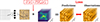 |
Fig. 1. Overview of NeuralBD deconvolution pipeline. The neural network maps coordinate points to pixel intensity values to estimate the real object intensity distribution. The convolution is calculated between the estimated real object and the predicted k PSFs, which are parameterized as learnable values on a grid. The optimization is performed between the predicted image burst and the original image burst from the telescope. |
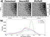 |
Fig. 2. (a) Comparison of a single frame of the burst from the degraded simulation (left), the NeuralBD reconstruction (center), and the real simulation (right). (b) Histogram of the normalized intensity for the convolved frame (green), the NeuralBD reconstruction (red), and the real simulation (blue). |
Figure 3 shows smaller cropped images of the single frame of the burst, the NeuralBD reconstruction, and the real simulation of Fig. 2. Additionally, we visualize the PSD for each of the crops. The lower panels show the power spectra for the single frame of the burst (green), the NeuralBD reconstruction (red), and the ground-truth simulation (black) as a function of spatial frequency. The power spectra of the NeuralBD reconstruction closely match those of the real simulation for both crops. Despite the strong overall agreement, small deviations can be seen in the spatial frequency range from 1 to 3 Mm−1, corresponding to the reconstruction performance of mid-sized structures.
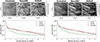 |
Fig. 3. Comparison of degraded convolved frame (left), the NeuralBD reconstruction (center), and the real simulation (right) for the quiet Sun and penumbra and umbra with penumbra. The bottom panel shows the corresponding power spectra density (PSD) for the convolved frame (green), the NeuralBD reconstruction (red), and the real simulation (black). |
Since the ground-truth PSFs are available for the reconstruction in Fig. 2, we can directly compare them with those estimated by our NeuralBD method. Figure 4 illustrates the effectiveness of our model in recovering accurate PSFs. The top row shows an example of the first five ground-truth PSFs used to degrade the simulation before training, while the bottom row shows the corresponding PSFs estimated by the NeuralBD model. The estimated PSFs closely resemble the ground truth in terms of their overall structure and features, demonstrating the model’s ability to produce realistic solutions. There are small differences on the smaller scales, as the NeuralBD PSFs look smoother. The reason for this is the intialization of the PSF as a Gaussian distribution. NeuralBD can also be initialized using the Karhunen–Loéve polynomials as basis functions and estimate the wavefront coefficients to obtain the exact solution. However, the PSF is always learned in the image domain, without any constraints independent of predefined wavefront coefficients. For initialization, we used a Gaussian distribution, but the model has the freedom to converge to any solution. The results shown in Fig. 4 demonstrate that our NeuralBD method can effectively handle the additional degree of freedom to estimate both the real object-intensity distribution and the PSFs by using just a Gaussian distribution as the initialization.
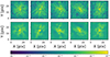 |
Fig. 4. Comparison of five PSFs initialized to degrade the synthetic MURaM simulation (top panel) and the PSF estimation by our NeuralBD model (bottom panel). |
In Fig. 5, we compare the reconstruction performance of our NeuralBD method to that of a standard reconstruction method using the Richardson–Lucy deconvolution and the torchmfbd method. Figure 5a) shows a clear improvement of the reconstructed observations for NeuralBD, Richardson–Lucy, and torchmfbd compared to the single convolved frame. However, comparing NeuralBD, Richardson–Lucy, and torchmfbd to the ground-truth MURaM simulation, NeuralBD shows a much closer resemblance to the simulation. Richardson-Lucy has much higher contrast and shows small scale artifacts in the reconstruction. On the other hand, torchmfbd shows a less sharp reconstruction compared to NeuralBD. This is also confirmed by the difference maps in Fig. 5b). The difference between NeuralBD and the ground-truth MURaM simulation (left) is much lower compared to the difference between the Richardson–Lucy deconvolution and the MURaM simulation (center) and the difference between torchmfbd and MURaM (right). The color bar represents the relative percentage difference. This is also confirmed by Table 1, where we see that NeuralBD outperforms both Richardson–Lucy and torchmfbd in all three quality metrics, including both distortion and perceptual metrics. The 2D histogram in Fig. 5c) also demonstrates the close resemblance of the NeuralBD reconstruction to the MURaM simulation compared to the Richardson–Lucy deconvolution and the torchmfbd method. It is important to note that the baseline method uses a single ground-truth PSF for deconvolution. In contrast, our NeuralBD approach estimates the PSFs and the reconstructed observation simultaneously during training, which makes the task considerably more challenging, yet it yields better results. Additionally, the torchmfbd method requires the information of the size of the telescope aperture and the wavelength for the reconstruction. Both parameters are not available since we used a MURaM simulation as ground truth. Consequently, we tested different configurations of telescope aperture and wavelength, and we found that an aperture of 5 m and a wavelength of 450 nm give the best results. An exhaustive hyperparameter search could further improve the reconstructions. To complete the evaluation, Fig. 5d) shows the PSD for the convolved frame, the MURaM simulation, the NeuralBD reconstruction, the Richardson–Lucy deconvolution, and the torchmfbd method. Here, Richardson–Lucy deconvolution and NeuralBD show close similarity with the simulation, outperforming the degraded frame. The reduced power of the torchmfbd method can be caused by the missing information of the telescope aperture and the wavelength. Note that the Richardson–Lucy deconvolution uses only one frame for reconstruction, whereas NeuralBD and torchmfbd use 50 frames and NeuralBD uses the PSFs estimated by the neural network.
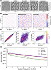 |
Fig. 5. Comparison of baseline method (Richardson–Lucy), torchmfbd method, and our NeuralBD reconstruction for MURaM simulation data. In panel (a), we show a visual comparison of a single convolved frame, the MURaM simulation, the NeuralBD reconstruction, the Richardson–Lucy deconvolution, and torchmfbd. Panel (b) shows the difference maps of our NeuralBD method, the baseline method, and torchmfbd. Panel (c) shows the 2D histograms comparing NeuralBD with MURaM (left), Richardson–Lucy with MURaM (center), and torchmfbd with MURaM (right). In panel (d), the power spectral density (PSD) for all five observations in (a) are shown. |
4.2. Application to GREGOR data
To demonstrate the reconstruction performance of our NeuralBD model on real high-resolution observations, we applied it to data from the 1.5 m GREGOR telescope and compared our NeuralBD reconstructions to state-of-the-art speckle reconstructions (Kuckein et al. 2017) and multi-frame blind deconvolutions. Fig. 6a) shows observations from June 2, 2022 in the g Band at 430.7 nm and blue continuum at 450.6 nm, respectively. The first column for each wavelength corresponds to a single frame with the best RMS contrast of the original image burst, the second column corresponds to the speckle reconstruction, the third column corresponds to the torchmfbd reconstruction, and the fourth column corresponds to our NeuralBD reconstruction. In the second and third rows, we show smaller crops marked by the red and blue boxes. For comparison, we shifted the NeuralBD reconstruction to match the mean value of the speckle reconstruction. This adjustment is necessary because the speckle reconstruction incorporates an atmospheric model with the speckle transfer function to estimate true intensities, whereas the NeuralBD reconstruction does not. However, such a correction can be applied afterwards. NeuralBD, speckle, and the torchmfbd reconstructions all show a clear improvement in sharpness compared to the original single frame. On the largest scales, NeuralBD, speckle, and the torchmfbd reconstructions demonstrate similar image quality. However, when zooming in on smaller scales (red box), NeuralBD reveals finer, more detailed structures within the bright points for both wavelength bands. On sub-arcsec scales (blue box), NeuralBD reveals features that are visible in the original frame, but remain unresolved and appear blurred in speckle and the torchmfbd reconstructions.
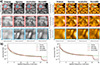 |
Fig. 6. Comparison of performance of the NeuralBD reconstruction method with the speckle and torchmfbd reconstructions for g band at 430.7 nm (left) and blue continuum at 450.6 nm (right). (a) Single frame from the original burst (first column), the speckle reconstruction (second column), the torchmfbd reconstruction (third column), and the NeuralBD reconstruction (fourth column) for the GREGOR observation on June 2, 2022. The red and blue rectangles indicate the cropped regions shown in the second and third rows, respectively. (b) Corresponding azimuthal power spectra for both channels are shown. The single frame of the original burst (green), the speckle reconstruction (black), the torchmfbd reconstruction (brown), and the NeuralBD reconstruction (red). |
In Fig. 6b), we show the corresponding PSD evaluations for the single frame, the speckle reconstruction, the torchmfbd reconstruction, and the NeuralBD reconstruction. All three reconstructions outperform single-frame data with torchmfbd and speckle showing similar power, slightly enhanced compared to NeuralBD. The blue continuum reconstruction performs better than the G-band reconstruction and even yields more power than the speckle reconstruction in the spatial frequency range from 10 to 14 arcsec−1. However, within the 4 to 9 arcsec−1 spatial frequency range, the speckle reconstruction shows slightly higher power in both filter bands. The feature around 25 arcsec−1 in both wavelength bands where the power suddenly drops corresponds to the diffraction limit of the telescope.
Figure 7 shows five representative examples of the first five frames from the 50 PSFs estimated by our NeuralBD model. The first row shows the PSFs estimated for the g band, and the second row shows the PSFs for the blue continuum. The overall structure of the PSFs are very similar in both bands, suggesting that a unique solution exists despite the large degree of freedom of the modeled PSFs. Additionally, the PSFs show a significant amount of jittering which cannot be modeled simply using wavefront coefficients. This is also confirmed in the last column, which shows the average PSF calculated over all estimated 50 PSFs from the NeuralBD model. However, there are small differences visible on smaller scales, which can be caused by the difference in the two filters that observe the same scene. Solving Eq. (1) in the image domain also allows for the construction of arbitrary PSFs, including spatial shifts, and is essential for extending the approach to spatially varying PSFs.
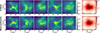 |
Fig. 7. Comparison of first five PSFs at 430.7 nm (G-Band) in the first row and 450.6 nm (Blue continuum) in the second row, as estimated by our NeuralBD model. The last column corresponds to the mean PSF calculated over the 50 PSFs from the NeuralBD model. |
4.3. Application to DKIST data
As a second high-resolution observation application, we tested our NeuralBD method on data from the VBI instrument on DKIST and compare our NeuralBD reconstruction with state-of-the-art, multi-frame blind deconvolutions and speckle reconstructions. Fig. 8a) shows the comparison of a single frame of the original burst (first column), the speckle reconstruction (second column), the torchmfbd reconstruction (third column), and our NeuralBD reconstruction (fourth column). The 5.5″ × 5.5″ cutout of the observation shows umbra and penumbra regions. In the second and third rows we show smaller cropped views, zooming in on penumbral structures up to sub-arcsecond scales. In comparing the single frame of the burst with the best RMS contrast value, the speckle reconstruction, the torchmfbd reconstruction, and the NeuralBD reconstruction one can see a clear improvement in the reconstructed observations. The cutouts in the red and green boxes confirm this on different spatial scales. Zooming in on sub-arcsec scales in the green box, NeuralBD shows fine-detail structures in the penumbra that cannot be fully resolved by the speckle reconstruction due to noise as well as for the torchmfbd reconstruction.
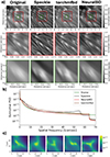 |
Fig. 8. Comparison of reconstruction methods with NeuralBD, torchmfbd, and speckle. (a) Single frame of the original burst (first column), the speckle reconstruction (second column), the torchmfbd reconstruction (third column), and the NeuralBD reconstruction (fourth column). The red and green boxes show zoomed-in views of the regions on smaller spatial scales. (b) The azimuthal power spectra are shown, where the green line corresponds to the single frame of the burst, black to the speckle reconstruction, brown to the torchmfbd reconstruction, and red to the NeuralBD reconstruction. (c) Five example PSFs estimated by the NeuralBD method. |
Figure 8b) compares the PSD for the single frame of the burst, the speckle reconstruction, the torchmfbd reconstruction, and the NeuralBD reconstruction. All three reconstructions show more power compared to the single frame of the burst. NeuralBD closely follows the green line from the single frame of the burst, suggesting that the seeing was good for this observation. Speckle, however, shows higher power in the range from 5 arcsec−1 to 12 arcsec−1, reaching a level similar to that of NeuralBD at around 13 arcsec−1. At around 40 arcsec−1, the power of speckle reconstruction starts rising, peaking at around 55 arcsec−1. This feature is likely caused by noise amplification due to insufficient noise filtering during the speckle reconstruction process. The torchmfbd reconstruction shows higher power starting from around 2 arcsec−1, consistently outperforming the original frame, speckle, and NeuralBD. The drop in the power at 65 arcsec−1 corresponds to the diffraction limit of the telescope.
In Fig. 8c), we show five example PSFs estimated from the NeuralBD method. They correspond to the five frames with the best RMS contrast value. The overall structure looks similar to the PSFs estimated for the GREGOR observations in Fig. 7. The PSFs exhibit structured features near their boundaries, suggesting that increasing the PSF size could be beneficial. However, increasing the PSF size would come at the cost of higher memory consumption and longer reconstruction times. Nevertheless, Fig. 8 shows that the NeuralBD reconstruction method achieves comparable results to the speckle one, while resolving small-scale features slightly more effectively with less noise.
5. Uncertainty estimation
To assess the uncertainty of our NeuralBD model, we trained five models with identical configurations using the GREGOR observations as described in Sect. 3.2 and Sect. 4.2. In Fig. 9a), we show the NeuralBD reconstruction for the five models. The last column corresponds to the uncertainty map showing the standard deviation (in percent) of the five reconstructions. The reconstructions are visually similar, with consistent large- and small-scale structures across all five runs. The uncertainty map shows only minor variations in the penumbral structures. Figure 9b) shows five example PSFs from the five different runs. The last row shows the uncertainty map, computed as the standard deviation (in percent) over all 100 PSFs for each of the five runs. The PSFs show similar global structures across all five runs, indicating that the model converges to a similar solution. The uncertainty maps show only small differences between the runs, even though the the overall PSF shapes are nearly identical. These differences are primarily due to sub-pixel spatial shifts of the PSFs, which are also visible in the uncertainty maps. This also explains the small differences in the uncertainty map in the reconstruction in Fig. 9a).
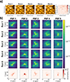 |
Fig. 9. Uncertainty estimation of NeuralBD model on five individual reconstruction runs using the GREGOR observation. a) NeuralBD reconstruction for the five different runs. The last column corresponds to the standard deviation of the five reconstructions in percent. b) Five example PSFs for the five different runs. The last row corresponds to the standard deviation evaluated for each of the five PSFs per run. |
6. Discussion
In this study, we developed an image-deconvolution method to reconstruct high-resolution ground-based solar observations. The method is based on PINNs and it calculates the real object-intensity distribution and the PSFs responsible for the distortions in the observations at the same time. By forward modeling, we solved the image equation (Eq. 1) to update the intensity values and the PSF parameters. Using this approach of neural representation can lead to smoother reconstructions with less noise (Tancik et al. 2020; Jarolim et al. 2025). Our method can be directly applied to any high-resolution broadband imaging instruments for ground-based solar observations and has no constraints for telescope aperture and wavelength.
We evaluated our NeuralBD method on simulation data to directly compare the reconstruction performance (see Fig. 2) and the estimation of the PSFs by our method (Fig. 4). Comparing the NeuralBD method to a baseline method and a multi-frame blind-deconvolution method, the NeuralBD reconstruction clearly outperforms the baseline one both visually (see Fig. 5) and in terms of perceptual and distortion quality metrics, as shown in Tale 1. Although NeuralBD must infer the PSFs as part of the reconstruction, it achieves higher performance than the baseline method, which benefits from a known ground-truth PSF. In contrast to the MFBD and MOMFBD approaches, NeuralBD does not make any assumptions about the PSFs, such as predefined basis functions or wavefront parameters (Van Noort et al. 2005; Asensio Ramos et al. 2018, 2023; Asensio Ramos 2024). This flexibility enables the model to reconstruct the optimal PSFs and, consequently, the most accurate representation of the real object. Compared to previous image-reconstruction methods, NeuralBD acts as a solver method and is therefore independent of a high quality data set. Additionally, this makes it independent of the application to any instrument.
A reconstruction of high-resolution observations from the 1.5 m GREGOR and 4 m DKIST solar telescopes demonstrated the independent applicability of NeuralBD to different instruments. When compared with state-of-the-art speckle reconstructions and multi-frame blind deconvolution, the NeuralBD results reveal finer details and better resolve small-scale features, with reduced noise on the smallest spatial scales due to the smooth image representation provided by the PINN (Jarolim et al. 2025). A comparison of the PSFs derived from the GREGOR observations in Fig. 7 shows that the NeuralBD method converges toward a unique physical solution, as the PSFs at both wavelengths exhibit similar structural features. This is also confirmed by Fig. 9, where five individual runs show similar performance in the reconstruction as well as close resemblance in the estimated PSFs. Nevertheless, the PSFs derived using NeuralBD differ significantly from the assumed PSFs from MFBD and MOMFBD, which suggests that this additional degree of freedom is essential for accurately modeling the imaging process (Asensio Ramos et al. 2023; Asensio Ramos 2024).
By directly solving the image-formation equation (Eq. 1) in the image domain, NeuralBD infers a PSF at each wavelength. This provides several advantages. First, chromatic effects can be handled naturally by estimating wavelength-dependent PSFs. Second, the approach can flexibly accommodate a wide range of image degradations and represent complex PSF structures that are difficult to capture with the parameterization using wavefronts. However, working directly in the image domain also has limitations. Unlike wavefront-based parameterizations, the inferred PSFs are not inherently constrained by physical optics. Initializing the PSFs with wavefronts automatically enforces properties such as positivity, normalization, and trivial wavelength scaling. Additionally, they often provide a more compact representation of the PSF if they are dominated by diffraction effects. Furthermore, the large contributions near the PSF boundaries visible in Fig. 8 indicate that increasing the PSF size could further improve the reconstructions, which requires more memory and, consequently, longer reconstruction times. Wavefront parameterizations can also have inherent limitations. They can struggle to capture effects of phase distortions, such as jittering or other non-diffraction-driven degradations. Moreover, ambiguities arise because different wavefront configurations can produce very similar PSFs, which can complicate the optimization and, therefore, the reconstruction performance. Solving Eq. (1) in the image domain and thus directly estimating the PSFs offers greater flexibility to find an optimal solution, while wavefront-based approaches provide stronger physical constraints and compactness.
The NeuralBD method is currently limited by the assumption of isoplanatic conditions, which restrict the reconstruction to a small FOV. To reconstruct a larger FOV, one can apply mosaicing of the individual patches. In future studies, we will explore pixel-wise, spatially variant PSFs to reconstruct the entire FOV of the observations (see Asensio Ramos 2024). Currently, the reconstruction process takes ∼7 hours on an NVIDIA A100 GPU. In future, we plan to investigate strategies to accelerate this process. This could involve patch-based sampling of the coordinate points, or initializing the network from a pre-trained meta state in order to reduce the time required to reconstruct subsequent observations.
This study demonstrates that NeuralBD can provide high-resolution solar-image reconstruction and exceed the performance to state-of-the-art reconstruction methods in terms of spatial resolution and noise mitigation. Since we have no constraints on telescope aperture, we can apply the method to any large-aperture ground-based solar telescope such as the GREGOR telescope, the Swedish solar telescope (SST; Scharmer et al. 2003), DKIST, and the future EST. This study lays the foundation for spatially varying PSFs and has the potential to be extended to other ground-based observations such as spectropolarimetric data.
Data availability
All codes are publicly available: Zenodo: Schirninger & Jarolim (2026) and GitHub: https://github.com/Schirni/NeuralBD
Acknowledgments
We thank the referee for very useful comments, which helped to improve the paper. This research has received financial support from the University of Graz EST (European Solar Telescope) program. The research was sponsored by the DynaSun project and has thus received funding under the Horizon Europe programme of the European Union under grant agreement (no. 101131534). Views and opinions expressed are however those of the author(s) only and do not necessarily reflect those of the European Union and therefore the European Union cannot be held responsible for them. RJ was supported by the NASA Jack-Eddy Fellowship. We acknowledge the use of the Vienna Scientific Cluster (VSC) for the computational resources and obtaining the results presented in this paper. This material is based upon work supported by the NSF National Center for Atmospheric Research (NCAR), which is a major facility sponsored by the U.S. National Science Foundation under Cooperative Agreement No. 1852977. The 1.5-meter GREGOR solar telescope was built by a German consortium under the leadership of the Institute for Solar Physics (KIS) in Freiburg with the Leibniz Institute for Astrophysics Potsdam, the Institute for Astrophysics Göttingen, and the Max Planck Institute for Solar System Research in Göttingen as partners, and with contributions by the Instituto de Astrofísica de Canarias and the Astronomical Institute of the Academy of Sciences of the Czech Republic. The research reported herein is based in part on data collected with DKIST a facility of the National Science Foundation. DKIST is operated by the National Solar Observatory under a cooperative agreement with the Association of Universities for Research in Astronomy, Inc. DKIST is located on land of spiritual and cultural significance to Native Hawaiian people. The use of this important site to further scientific knowledge is done so with appreciation and respect. We thank Christoph Kuckein for providing us with the speckle reconstructions from the GREGOR telescope and Friedrich Wöger for providing us the DKIST data. This research has made use of AstroPy (Astropy Collboration 2022), SunPy (Barnes 2020) and PyTorch (Paszke et al. 2017).
References
- Asensio Ramos, A. 2024, A&A, 688, A88 [NASA ADS] [CrossRef] [EDP Sciences] [Google Scholar]
- Asensio Ramos, A., de la Cruz Rodríguez, J., & Pastor Yabar, A. 2018, A&A, 620, A73 [NASA ADS] [CrossRef] [EDP Sciences] [Google Scholar]
- Asensio Ramos, A., Esteban Pozuelo, S., & Kuckein, C. 2023, Sol. Phys., 298, 91 [Google Scholar]
- Asensio Ramos, A., Löfdahl, M. G., Díaz Baso, C., Kuckein, C., & Esteban Pozuelo, S. 2025, A&A, 703, A269 [NASA ADS] [CrossRef] [EDP Sciences] [Google Scholar]
- Astropy Collboration (Price-Whelan, A. M., et al.) 2022, ApJ, 935, 167 [NASA ADS] [CrossRef] [Google Scholar]
- Beard, A., Wöger, F., & Ferayorni, A. 2020, SPIE Conf. Ser., 11452, 114521X [Google Scholar]
- de Boer, C. R., & Kneer, F. 1992, A&A, 264, L24 [NASA ADS] [Google Scholar]
- Denker, C., Verma, M., Wiśniewska, A., et al. 2023, J. Astron. Telescopes Instrum. Syst., 9, 015001 [NASA ADS] [Google Scholar]
- Díaz Baso, C. J., Asensio Ramos, A., de la Cruz Rodríguez, J., da Silva Santos, J. M., & Rouppe van der Voort, L. 2025, A&A, 693, A170 [NASA ADS] [CrossRef] [EDP Sciences] [Google Scholar]
- Fardo, F. A., Conforto, V. H., de Oliveira, F. C., & Rodrigues, P. S. 2016, ArXiv preprint [arXiv:1605.07116] [Google Scholar]
- Goodfellow, I., Pouget-Abadie, J., Mirza, M., et al. 2020, Commun. ACM, 63, 139 [CrossRef] [Google Scholar]
- Jarolim, R., Molnar, M. E., Tremblay, B., Centeno, R., & Rempel, M. 2025, ApJ, 985, L7 [Google Scholar]
- Jarolim, R., Thalmann, J. K., Veronig, A. M., & Podladchikova, T. 2023, Nat. Astron., 7, 1171 [NASA ADS] [CrossRef] [Google Scholar]
- Jarolim, R., Tremblay, B., Muñoz-Jaramillo, A., et al. 2024, ApJ, 961, L31 [NASA ADS] [Google Scholar]
- Karniadakis, G. E., Kevrekidis, I. G., Lu, L., et al. 2021, Nat. Rev. Phys., 3, 422 [Google Scholar]
- Knox, K. T., & Thompson, B. J. 1974, ApJ, 193, L45 [Google Scholar]
- Kuckein, C., Denker, C., Verma, M., et al. 2017, IAU Symp., 327, 20 [NASA ADS] [Google Scholar]
- Labeyrie, A. 1970, A&A, 6, 85 [Google Scholar]
- Löfdahl, M. G., Bones, P. J., & Millane, R. P. 2002, SPIE, 4792, 146 [Google Scholar]
- Löfdahl, M. G., & Scharmer, G. B. 1994, A&AS, 107, 243 [NASA ADS] [Google Scholar]
- Löfdahl, M. G., & Scharmer, G. B. 2003, Proc. SPIE, 4853, 567 [Google Scholar]
- Löfdahl, M. G., van Noort, M. J., & Denker, C. 2006, in Modern Solar Facilities - Advanced Solar Science, eds. F. Kneer, K. G. Puschmann, & A. D. Wittmann (Göttingen, Germany: Universitätsverlag Göttingen), 119 [Google Scholar]
- Lohmann, A. W., Weigelt, G., & Wirnitzer, B. 1983, Appl. Opt., 22, 4028 [NASA ADS] [CrossRef] [Google Scholar]
- McKechnie, T. S. 1992, J. Opt. Soc. Am. A, 9, 1937 [Google Scholar]
- Paszke, A., Gross, S., Chintala, S., et al. 2017, NIPS-W [Google Scholar]
- Priest, E. R., & Forbes, T. 2002, A&ARv, 10, 313 [Google Scholar]
- Quintero Noda, C., Schlichenmaier, R., Bellot Rubio, L. R., et al. 2022, A&A, 666, A21 [NASA ADS] [CrossRef] [EDP Sciences] [Google Scholar]
- Quirrenbach, A. 2006, A. Extrasolar planets. Saas-Fee Advanced Course, 31, 137 [Google Scholar]
- Raissi, M., Perdikaris, P., & Karniadakis, G. E. 2019, J. Comput. Phys., 378, 686 [NASA ADS] [CrossRef] [Google Scholar]
- Rempel, M. 2017, ApJ, 834, 10 [Google Scholar]
- Rempel, M., & Cheung, M. C. M. 2014, ApJ, 785, 90 [Google Scholar]
- Richardson, W. H. 1972, J. Opt. Soc. Am. (1917–1983), 62, 55 [Google Scholar]
- Rimmele, T., Hegwer, S., Richards, K., & Woeger, F. 2008, in Advanced Maui Optical and Space Surveillance Technologies Conference, eds. C. Paxson, H. Snell, J. Griffin, et al., E18 [Google Scholar]
- Rimmele, T. R., & Marino, J. 2011, Liv. Rev. Sol. Phys., 8, 2 [Google Scholar]
- Rimmele, T. R., Warner, M., Keil, S. L., et al. 2020, Sol. Phys., 295, 172 [Google Scholar]
- Scharmer, G. B., Bjelksjo, K., Korhonen, T. K., Lindberg, B., & Petterson, B. 2003, SPIE Conf. Ser., 4853, 341 [NASA ADS] [Google Scholar]
- Schirninger, C., & Jarolim, R. 2026, https://doi.org/10.5281/zenodo.18471596 [Google Scholar]
- Schirninger, C., Jarolim, R., Veronig, A. M., & Kuckein, C. 2025, A&A, 693, A6 [NASA ADS] [CrossRef] [EDP Sciences] [Google Scholar]
- Schmidt, W., von der Lühe, O., Volkmer, R., et al. 2012, Astron. Nachr., 333, 796 [Google Scholar]
- Schulz, T. J. 1993, J. Opt. Soc. Am. A, 10, 1064 [NASA ADS] [CrossRef] [Google Scholar]
- Sitzmann, V., Martel, J., Bergman, A., Lindell, D., & Wetzstein, G. 2020, Adv. Neural Inf. Proc. Syst., 33, 7462 [Google Scholar]
- Tancik, M., Srinivasan, P., Mildenhall, B., et al. 2020, Adv. Neural Inf. Proc. Syst., 33, 7537 [Google Scholar]
- The SunPy Community (Barnes, W. T., et al.) 2020, ApJ, 890, 68 [Google Scholar]
- Van Noort, M., Rouppe Van Der Voort, L., & Löfdahl, M. G. 2005, Sol. Phys., 228, 191 [NASA ADS] [CrossRef] [Google Scholar]
- von der Luehe, O. 1984, J. Opt. Soc. Am. A, 1, 510 [CrossRef] [Google Scholar]
- Wang, Z., Bovik, A. C., Sheikh, H. R., & Simoncelli, E. P. 2004, IEEE Trans. Image Proc., 13, 600 [CrossRef] [Google Scholar]
- Wiegelmann, T., Thalmann, J. K., & Solanki, S. K. 2014, A&ARv, 22, 78 [Google Scholar]
- Wöger, F., Rimmele, T., Ferayorni, A., et al. 2021, Sol. Phys., 296, 145 [CrossRef] [Google Scholar]
- Wöger, F., von der Lühe, O., & Reardon, K. 2008, A&A, 488, 375 [NASA ADS] [CrossRef] [EDP Sciences] [Google Scholar]
- Wöger, F., von der Lühe, I. I. O. 2008, SPIE Conf. Ser., 7019, 70191E [Google Scholar]
All Tables
Comparison of quality metrics between the baseline (Richardson–Lucy) the torchmfbd and our NeuralBD model against the MURaM simulation.
All Figures
|
Fig. 1. Overview of NeuralBD deconvolution pipeline. The neural network maps coordinate points to pixel intensity values to estimate the real object intensity distribution. The convolution is calculated between the estimated real object and the predicted k PSFs, which are parameterized as learnable values on a grid. The optimization is performed between the predicted image burst and the original image burst from the telescope. |
| In the text | |
|
Fig. 2. (a) Comparison of a single frame of the burst from the degraded simulation (left), the NeuralBD reconstruction (center), and the real simulation (right). (b) Histogram of the normalized intensity for the convolved frame (green), the NeuralBD reconstruction (red), and the real simulation (blue). |
| In the text | |
|
Fig. 3. Comparison of degraded convolved frame (left), the NeuralBD reconstruction (center), and the real simulation (right) for the quiet Sun and penumbra and umbra with penumbra. The bottom panel shows the corresponding power spectra density (PSD) for the convolved frame (green), the NeuralBD reconstruction (red), and the real simulation (black). |
| In the text | |
|
Fig. 4. Comparison of five PSFs initialized to degrade the synthetic MURaM simulation (top panel) and the PSF estimation by our NeuralBD model (bottom panel). |
| In the text | |
|
Fig. 5. Comparison of baseline method (Richardson–Lucy), torchmfbd method, and our NeuralBD reconstruction for MURaM simulation data. In panel (a), we show a visual comparison of a single convolved frame, the MURaM simulation, the NeuralBD reconstruction, the Richardson–Lucy deconvolution, and torchmfbd. Panel (b) shows the difference maps of our NeuralBD method, the baseline method, and torchmfbd. Panel (c) shows the 2D histograms comparing NeuralBD with MURaM (left), Richardson–Lucy with MURaM (center), and torchmfbd with MURaM (right). In panel (d), the power spectral density (PSD) for all five observations in (a) are shown. |
| In the text | |
|
Fig. 6. Comparison of performance of the NeuralBD reconstruction method with the speckle and torchmfbd reconstructions for g band at 430.7 nm (left) and blue continuum at 450.6 nm (right). (a) Single frame from the original burst (first column), the speckle reconstruction (second column), the torchmfbd reconstruction (third column), and the NeuralBD reconstruction (fourth column) for the GREGOR observation on June 2, 2022. The red and blue rectangles indicate the cropped regions shown in the second and third rows, respectively. (b) Corresponding azimuthal power spectra for both channels are shown. The single frame of the original burst (green), the speckle reconstruction (black), the torchmfbd reconstruction (brown), and the NeuralBD reconstruction (red). |
| In the text | |
|
Fig. 7. Comparison of first five PSFs at 430.7 nm (G-Band) in the first row and 450.6 nm (Blue continuum) in the second row, as estimated by our NeuralBD model. The last column corresponds to the mean PSF calculated over the 50 PSFs from the NeuralBD model. |
| In the text | |
|
Fig. 8. Comparison of reconstruction methods with NeuralBD, torchmfbd, and speckle. (a) Single frame of the original burst (first column), the speckle reconstruction (second column), the torchmfbd reconstruction (third column), and the NeuralBD reconstruction (fourth column). The red and green boxes show zoomed-in views of the regions on smaller spatial scales. (b) The azimuthal power spectra are shown, where the green line corresponds to the single frame of the burst, black to the speckle reconstruction, brown to the torchmfbd reconstruction, and red to the NeuralBD reconstruction. (c) Five example PSFs estimated by the NeuralBD method. |
| In the text | |
|
Fig. 9. Uncertainty estimation of NeuralBD model on five individual reconstruction runs using the GREGOR observation. a) NeuralBD reconstruction for the five different runs. The last column corresponds to the standard deviation of the five reconstructions in percent. b) Five example PSFs for the five different runs. The last row corresponds to the standard deviation evaluated for each of the five PSFs per run. |
| In the text | |
Current usage metrics show cumulative count of Article Views (full-text article views including HTML views, PDF and ePub downloads, according to the available data) and Abstracts Views on Vision4Press platform.
Data correspond to usage on the plateform after 2015. The current usage metrics is available 48-96 hours after online publication and is updated daily on week days.
Initial download of the metrics may take a while.