| Issue |
A&A
Volume 709, May 2026
|
|
|---|---|---|
| Article Number | A14 | |
| Number of page(s) | 14 | |
| Section | Extragalactic astronomy | |
| DOI | https://doi.org/10.1051/0004-6361/202558073 | |
| Published online | 30 April 2026 | |
Gas excitation of post-SB galaxies at 0.6 < z < 1.3
1
Istituto Nazionale di Astrofisica (INAF), Via Gobetti 93/3, 40129 Bologna, Italy
2
Dipartimento di Fisica e Astronomia, Università di Bologna, Italy
3
Cosmic Dawn Center (DAWN), Denmark
4
DTU Space, Technical University of Denmark, Elektrovej 327, DK-2800 Kgs. Lyngby, Denmark
5
Max-Planck-Institut für Astrophysik, Karl-Schwarzschild-Str. 1, D-85748 Garching, Germany
6
INAF – IASF Milano, Via A. Corti 12, I-20133 Milano, Italy
★ Corresponding author: This email address is being protected from spambots. You need JavaScript enabled to view it.
Received:
11
November
2025
Accepted:
12
March
2026
Abstract
Context. Molecular gas in galaxies traces both the fuel for star formation and the processes that enhance or suppress it. Observing its physical state (e.g., excitation) can reveal when and why galaxies stop forming stars.
Aims. We observed the CO(5–4) emission of eight post-SB galaxies at z ∼ 0.6 − 1.3. To our knowledge, this is the first time that high-J transitions have been probed for post-SB or quiescent galaxies beyond the local Universe. All of them have detections in lower-J CO transitions (either CO(2–1) or CO(3–2)) and molecular gas fractions up to ∼20%. By studying the ratio R52 = L′CO(5 − 4)/L′CO(2 − 1), a proxy for the gas excitation, we aim to constrain the physical state of the gas.
Methods. The CO excitation helps to distinguish among different mechanisms responsible for the low star formation efficiency (SFE) of post-SB galaxies. In the first scenario, the molecular gas is predominantly diffuse and cold, implying a low fraction of dense star-forming gas and in turn low R52 values. In the second scenario, elevated gas temperatures at moderate densities, for example due to active galactic nucleus (AGN) activity, shocks, or enhanced turbulence, would instead produce high R52 values.
Results. Our post-SBs have on average R52 = 0.28, comparable to high-redshift main-sequence galaxies. However, when considering only the CO(5–4) non-detections, which also coincide with post-starbusts that do not show signs of interaction, we obtain R52 < 0.10, twice lower than local star-forming galaxies and more than 2.5 times lower than high-redshift sources. The average CO spectral line energy distribution (SLED) peaks at J = 3, similar to the Milky Way. Three galaxies show signs of interactions (tidal features, companions). They have R52 = 0.40 and SLEDs peaking at J ≳ 4 − 5. In at least one case additional mechanisms (e.g., AGNs, shocks) are needed to explain the steep rise of the SLED up to J = 5.
Conclusions. Our results favor a scenario in which most systems are dominated by low-density molecular gas with low excitation, consistent with quenching driven by gas stabilization, feedback regulation, or stripping. In interacting systems instead, enhanced excitation is likely driven by heating processes not related to star formation (e.g., AGNs, turbulence, shocks). Residual star formation is insufficient to rapidly exhaust the remaining molecular gas in the majority of post-SB galaxies.
Key words: galaxies: evolution / galaxies: general / galaxies: ISM
© The Authors 2026
 Open Access article, published by EDP Sciences, under the terms of the Creative Commons Attribution License (https://creativecommons.org/licenses/by/4.0), which permits unrestricted use, distribution, and reproduction in any medium, provided the original work is properly cited.
This article is published in open access under the Subscribe to Open model. This email address is being protected from spambots. You need JavaScript enabled to view it. to support open access publication.
1. Introduction
Despite significant observational and theoretical efforts, the physical mechanisms quenching star formation remain under active investigation and are still a central challenge in our understanding of galaxy evolution. A plethora of different mechanisms have been proposed to stop star formation by either reducing or depleting the molecular gas reservoir or rendering the gas unable to cool and form stars (Man & Belli 2018). In particular, cold gas accretion onto the galaxy dark matter halo might be prevented (Larson et al. 1980; Feldmann & Mayer 2015; Peng et al. 2015; Feldmann et al. 2017; Davé et al. 2017) or the infalling gas might be heated up because of virial shocks (Rees & Ostriker 1977; Dekel & Birnboim 2006). In both cases, additional mechanisms are needed to prevent the cold gas reservoir that is already present in the galaxy from forming new stars and to keep the galaxy quiescent. Feedback-driven outflows from active galactic nuclei (AGNs) might expel the gas from the galaxy (quasar-mode feedback, Di Matteo et al. 2005) while inefficient accretion onto the supermassive back hole (radio-mode feedback) keeps the galaxy quenched by heating the gas (Bower et al. 2006; Croton et al. 2006; Hopkins et al. 2006). Other mechanisms that have been suggested are gravitational heating due to the energy released by ram-pressure stripping (Gunn et al. 1972; Werle et al. 2022) or dynamical friction (e.g., during the infall of a satellite or clump, Khochfar & Ostriker 2008). Gas might also be consumed by starbursts (SBs) possibly triggered by major mergers (Mihos & Hernquist 1996; Springel et al. 2005; Wellons et al. 2015) and disk instabilities (Zolotov et al. 2015). However, quenching might be due to a low SFE rather than due to the lack of fuel. The cold gas disk of galaxies might be stable against collapse and fragmentation due to the presence of a bulge (Martig et al. 2009; Johansson et al. 2009) or a stellar bar (Khoperskov et al. 2018).
Understanding what mechanisms are responsible for galaxy quenching requires identifying galaxies in the immediate aftermath of their final star-forming episode and accurately characterizing their cold gas content and physical conditions. Post-SB galaxies, also referred to as “k+a” or “e+a” systems, represent a promising population for probing this transition phase. These galaxies exhibit optical spectra dominated by strong Balmer absorption lines, indicative of A-type stars formed in a recent burst of star formation, coupled with weak or absent nebular emission lines, signaling little to no ongoing star formation (Dressler & Sandage 1983; Couch & Sharples 1987). Recent observations of low-J CO transitions such as CO(2–1) and CO(3–2), classical tracers of total cold molecular gas, have revealed significant molecular gas reservoirs in post-SB galaxies up to redshifts of z ∼ 1.4 (French et al. 2015; Rowlands et al. 2015; Suess et al. 2017; French et al. 2018; Belli et al. 2021; Bezanson et al. 2022; Zanella et al. 2023; Suess et al. 2025). These studies report a wide variety of gas fractions that can be as high as 20%, suggesting that substantial amounts of star-forming fuel can remain in galaxies after the cessation of star formation. Despite this, post-SBs appear to lie systematically below the star-forming galaxy population in the Kennicutt–Schmidt relation, implying that their low star formation rates (SFRs) are not due to a lack of gas, but rather to a suppression of SFE (Zanella et al. 2023). This interpretation, however, remains tentative due to two key uncertainties: the excitation correction factor required to convert CO line luminosities to total molecular gas masses, typically assumed to be 15–50%, based on values from star-forming galaxies; and the obscured SFR, which is often inferred from mid-infrared (e.g., 24 μm) emission. The latter can be significantly contaminated by dust heating from evolved stellar populations, particularly in post-SB systems (Leja et al. 2019; Belli et al. 2021), complicating the accurate measurement of residual star formation activity.
Probing denser and/or warmer molecular gas through CO(5–4) emission provides a key diagnostic of the excitation state of the molecular medium, commonly quantified via the ratios R52, R53 (i.e., L′CO54/L′CO21 and L′CO54/L′CO32, respectively). These ratios are sensitive to both gas density and kinetic temperature and can be used to assess if residual, possibly obscured star formation is present, or whether the molecular gas is predominantly diffuse and inefficient at forming stars. If large reservoirs of molecular gas traced by low-J CO transitions are unable to sustain star formation in post-SB galaxies, low R52 and R53 values are expected, indicating a small fraction of dense and/or warm gas relative to the cold, diffuse molecular component. Conversely, high excitation ratios comparable to those of main-sequence or SB galaxies may signal either the presence of dense, star-forming gas (implying a high SFE) or elevated gas temperatures driven by additional heating mechanisms such as merger-induced shocks, turbulence, or AGN activity. To date, however, observations of high-J CO transitions in post-SB or quenched galaxies remain scarce.
In the local Universe, French et al. (2023) constrained the CO spectral line energy distribution (SLED) of a sample of post-SB galaxies up to the CO(3–2) transition. They found low excitation, consistent with the low HCO+/CO ratios observed in the same galaxies, indicating that low fractions of dense molecular gas relative to the total molecular gas drive the reduced SFE in these systems. This sample partially overlaps with that of Smercina et al. (2022), who analyzed high-resolution CO(2–1) observations and found that the turbulent kinetic pressure of the gas exceeds that of typical star-forming disks, resembling instead the conditions in local interacting galaxies such as the Antennae. They suggest that this turbulence prevents the gas from collapsing, further contributing to the suppression of star formation. Constraining the CO excitation at higher redshift is therefore key to understand whether similar mechanisms drive the low SFE of post-SBs across redshift.
This paper is organized as follows: in Sect. 2 we describe the sample and the data; in Sect. 3 we discuss how we estimated the observables and derived physical properties; in Sect. 4 we present our results in the context of available literature; in Sect. 5 we discuss the possible mechanisms that keep our galaxies quiescent and the decoupling of molecular gas and dust; and in Sect. 6 we conclude and summarize our findings. Throughout the paper we adopt a flat Λ cold dark matter cosmology with Ωm = 0.3, ΩΛ = 0.7, and H0 = 70 km s−1 Mpc−1. All magnitudes are AB magnitudes (Oke 1974) and we adopt a Chabrier (2003) initial mass function.
2. Data
We focus on eight gas-rich post-SB galaxies at 0.6 < z < 1.3. They were all the publicly available (to our best knowledge) and observable by ALMA z ≳ 0.6 post-SBs with detected low-J CO (J = 2, 3) lines at the time when the observations were proposed (Suess et al. 2017; Bezanson et al. 2022; Zanella et al. 2023).
2.1. Sample selection and ancillary data
The sample was extracted from two surveys: SQuIGGLE (Suess et al. 2022) and the study of Zanella et al. (2023). The SQuIGGLE sample was selected from the Sloan Digital Sky Survey DR14 spectroscopic database (Abolfathi et al. 2018) to have strong Balmer breaks, blue slopes redward of the break, and z ∼ 0.7. For a description of the spectroscopic identification, stellar populations, and physical characterization of SQuIGGLE galaxies we refer the reader to the survey paper (Suess et al. 2022). A subset of the SQuIGGLE sample has been observed with ALMA targeting the CO(2–1) line emission (Suess et al. 2017; Bezanson et al. 2022). Of the 13 targeted galaxies, CO(2–1) emission was detected in six. These 6 galaxies are those we focus on in this study. We note that a more recent study targeted the CO(2–1) emission of 50 additional post-SBs detecting 27 of them (Setton et al. 2025). None of them have so far published data of higher-J CO transitions. However, our sample selection and observations were concluded before this study was published.
The galaxies from Zanella et al. (2023) were initially optically selected by Wild et al. (2016) applying a principal component analysis on their spectral energy distributions (SEDs) based on the photometry of the Ultra-Deep Survey (Lawrence et al. 2007). The post-SB nature of a subsample of 19 objects with deep absorption lines (EW(Hδ > 5 Å) and minimal [OII]3727 Å emission consistent with the unobscured SFR estimated from the UV luminosity was confirmed by Maltby et al. (2016). Two z > 1 targets from this subsample were targeted with ALMA by Zanella et al. (2023) and the CO(3–2) emission line was detected. In Table 1 we report the ALMA observations for our sample.
Log of the ALMA observations used in this work.
2.2. ALMA CO(5–4) data
We carried out ALMA Band 6 (for z < 1 sources) or 7 (for z > 1 sources) observations for our sample during Cycle 11 (Program 2024.1.00061, PI: A. Zanella) with the goal of detecting the CO(5–4) emission line at rest-frame frequency νrf = 576.267 GHz and the underlying continuum, redshifted in the frequency range νobs = 260 − 360 GHz. Each source was observed for 8–110 minutes. The sensitivities achieved are reported in Table 1. The native spectral resolution of the observations is 6.5–13.5 km s−1, later binned to three times lower velocity resolution for our purposes. The angular resolution of the observations is in the range 0.5″ − 1.4″ (Table 1).
The data were reduced with the standard ALMA pipeline, based on the CASA software (McMullin et al. 2007). The calibrated data cubes were then converted to uvfits format and analyzed with the software GILDAS (Guilloteau & Lucas 2000). For consistency, we also retrieved from the ALMA archive the publicly available low-J CO data and reduced them adopting the same procedure of our CO(5–4) observations.
3. Analysis
3.1. CO(5–4) emission
To produce the velocity-integrated CO(5–4) line maps for our targets, we first determined the optimal spectral range over which to integrate the spectra. This was done through an iterative procedure, following an approach similar to that described in Zanella et al. (2023). We modeled the emission in the uv plane1 as an elliptical Gaussian, fitting channel by channel across all four sidebands with the GILDAS task uv_fit. Our sources are expected to be unresolved and the size of the elliptical Gaussian is indeed consistent with the beam size. Nevertheless, we chose to adopt an extended model rather than a point source, to ensure consistency with the analysis of the low-J CO emission, which in several cases is spatially resolved (Section 3.2). We verified that using a point-source model yields CO(5–4) integrated fluxes and upper limits that are, on average, 1.5 times fainter. However, this difference does not affect our conclusions.
The spatial positions of the models were fixed to those derived from the CO(2–1) emission, which are consistent with the positions measured from optical imaging. Using these models, we extracted one-dimensional (1D) spectra and searched for positive line emission. When such a signal was detected, we averaged the channels that maximized the S/N (S/N), and used the resulting channel-averaged two-dimensional (2D) map to fit the spatial position of the line. We considered a galaxy to be detected if its peak flux reached a significance of at least 3σ. In addition, we verified that the redshift of the detected CO line is consistent with the spectroscopic redshift from optical data and that the CO emission is spatially consistent with the optical and IR emission. We estimated the total line flux by fitting a 1D Gaussian to the extracted optimal S/N spectrum. When a line was not detected, we instead created 2D maps using the channel range identified for the CO(2–1) emission and adopted a 3σ flux upper limit. We securely detected the CO(5–4) emission line for three galaxies, while the remaining are undetected (Fig. 1).
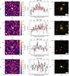 |
Fig. 1. ALMA data of our galaxies. First column: 2D maps of the CO(5–4) line. The solid and dashed cyan contours indicate, respectively, positive and negative levels of (2.5, 3.5, 4.5, 5.5) rms. The beam is reported in the bottom left corner (white ellipse). Each stamp has a size of 10″ × 10″. The cyan cross indicates the center of our post-SBs as estimated from the optical emission. Second column: 1D spectra of sources extracted using a PSF to maximize the signal-to-noise ratio (S/N). The shaded pink areas indicate the 1σ velocity range over which we measured the CO(5–4) line flux or its upper limit. For detections we also report the Gaussian fit of the emissions (Sect. 3.1). The vertical dashed lines indicate the observed frequency corresponding to the redshift of the low-J CO emission. Third column: Rest-frame optical grz images from the DESI Legacy Survey DR9 Dey et al. (2019). The cyan contours show the CO(5–4) emission, while the orange and pink indicate the low-J (CO(2–1) or CO(3–2)) or CO(4–3) emission, respectively. The ellipses indicate the beam size. Each stamp has a size of 20″ × 20″. The contour levels are the same as in the first panels. (Continues on page 6). |
To increase the S/N for non-detections we aligned the individual CO(5–4) maps to the CO(2–1) positions and stacked them (coadding visibilities). Even the stacking yielded a non-detections. We estimated a CO(5–4) flux upper limit by fitting the stacked data in the uv plane with the Fourier transform of a 2D Gaussian with parameters fixed to those obtained by stacking the CO(2–1) stacking.
We estimated the redshift of the three detected CO(5–4) lines in two ways, both giving consistent results (δz < 0.001): by computing the signal-weighted average frequency within the line channels and by fitting the 1D spectrum with a Gaussian function. We compared these redshift estimates with those obtained from CO(2–1) (Bezanson et al. 2022; Zanella et al. 2023) and found that they agree within the uncertainties. The CO(5–4) total fluxes and redshifts are reported in Table 2 (See Fig. 2).
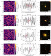 |
Fig. 2. ALMA data of our galaxies (continued). As reported in Bezanson et al. (2022), the ∼1″ offset of the CO(2–1) of J2202 from the optical centroid is not significant given the data resolution and S/N. However, we note that the optical image of this galaxy appears to be slightly asymmetric. |
Measurements for our sample galaxies.
3.2. Low-J CO emission
Since the main goal of this study is to compare the CO(5–4) and lower-J CO transitions, we reanalysed archival public data targeting the CO(2–1), CO(3–2), and/or CO(4–3) emission lines using the same procedure adopted for the CO(5–4) emission (Section 3.1). The fluxes we obtain are on average 20% fainter than those reported in the literature (Suess et al. 2017; Bezanson et al. 2022; Zanella et al. 2023), due to the different methodology used to extract the 1D spectra and measure fluxes. In our analysis, we adopt fixed elliptical apertures that are held constant across all velocity channels and across all datasets. In contrast, Suess et al. (2017) and Bezanson et al. (2022) adopt circular Gaussian models with radii that vary on a channel-by-channel basis. We prefer the fixed-aperture approach because it minimizes the impact of noise fluctuations in individual channels, and it ensures that exactly the same spatial region is used when measuring fluxes in different transitions, which is particularly important for robust line ratio measurements. We verified that using elliptical instead of circular Gaussian models yields negligible differences. The main difference with respect to the Zanella et al. (2023) dataset instead lies in the adopted source model. While Zanella et al. (2023) use a point-source model, motivated by the fact that the CO(3–2) transition appeared unresolved in their data, we adopt an elliptical Gaussian model. This choice is made to ensure methodological consistency with the analysis applied to the rest of our sample. Since the same apertures are applied consistently to all datasets, any systematic difference in the absolute flux normalization does not affect the derived line ratios. We report all fluxes in Table 2. A comparison of the spatial locations and morphologies of the different emission lines is shown in Figure 1.
3.3. Continuum emission
We generated averaged continuum maps by integrating over the spectral range. For the CO(5–4) detected galaxies, we excluded the channels dominated by line emission, while for the non-detections we excluded the channels where emission is expected based on the low-J CO transitions (see Section 3.2 for details). None of our main targets is detected in the νobs = 260–360 GHz continuum, down to sensitivities in the range 12.6 − 99.3 μJy. We also produced continuum maps by averaging over a broader spectral range, including not only the continuum underlying the CO(5–4) line but also that associated with the lower-J transitions. This analysis likewise yielded no detections, down to sensitivities in the range 4.5 − 21.0 μJy. Since no detections were found, we did not refine this analysis further, for example by assuming a continuum slope when stacking across different frequency ranges.
3.4. Detection of companion galaxies
Three of our sample galaxies have companions or tidal features that have been identified in low-J CO maps. We verified whether they are also detected in CO(5–4).
In particular, Zanella et al. (2023) serendipitously detected bright CO(3–2) emission lines (14.0σ and 16.5σ) and continuum (3.5σ and 4.7σ) from two galaxies in the surroundings of ID83492. Those galaxies are also detected in CO(5–4), despite having a lower significance (10.6σ and 5.5σ). They both have optical counterparts in Hubble Space Telescope Wide Field Camera 3 (HST/WFC3) imaging from the 3D-HST program (Skelton et al. 2014) and their CO(5–4) redshifts are z = 1.1377 ± 0.0002 and z = 1.1380 ± 0.0004, consistent with the CO(2–1) redshift (Δz ≲ 0.0003). Given their velocity offset (voff ∼ 250 km s−1 and voff ∼ 195 km s−1) and projected distance from ID83492 (5.8″ ∼ 48 kpc and 13.7″ ∼ 112 kpc), they are likely companions that might merge with our target galaxy within < 2.5 Gyr, as already reported by Zanella et al. (2023). We report the properties of all companions in Tables 2 and 3.
Physical properties of our sample galaxies.
Additionally, Spilker et al. (2022) and D’Onofrio et al. (2025) have analyzed spatially resolved CO(2–1) maps of the J1448 and J2258 galaxies, revealing extended molecular gas tidal tails spanning up to 65 kpc, a clear indication of recent mergers. Such extended tidal features are not detected in CO(5–4) likely due to the lack of sufficient sensitivity. Only a tentative (∼4σ) CO(5–4), spatially unresolved, emission emerges at the location of the Northern tail N3 identified by D’Onofrio et al. (2025) with CO(2–1) and Hα emission. Its CO(5–4) redshift (z = 0.6457 ± 0.0003) is consistent with that of the central body of J1448 (Table 2).
Finally, we searched for dust continuum detections nearby our targets. We report the detections in Appendix A, while coordinates and fluxes are reported in Table A.1.
3.5. Physical properties
Stellar masses and SFR were obtained by modeling multi-wavelength photometry as described in Bezanson et al. (2022) and Zanella et al. (2023). In brief, Bezanson et al. (2022) modeled the photometry and spectra simultaneously using Prospector (Leja et al. 2017) with a custom set of “nonparametric” star formation histories, assuming a Kriek & Conroy (2013) dust law2. Zanella et al. (2023) modeled the photometry and the spectra simultaneously with FAST++3 (Schreiber et al. 2018) using Bruzual & Charlot (2003) models, the Chabrier (2003) IMF, delayed SFHs, the Calzetti et al. (2000) dust attenuation curve, and fixed the redshifts to the spectroscopic values. We report the specific star formation rate sSFR = SFR/M★ in Table 3.
The molecular gas masses (MH2) were estimated from the CO(2–1) emission for the galaxies at z < 1 (Bezanson et al. 2022) and from the CO(3–2) line for the targets with z > 1 (Zanella et al. 2023). Both (Bezanson et al. 2022) and (Zanella et al. 2023) use a Milky Way-like CO-to-H2 conversion factor (Bolatto et al. 2013) and adopt the following excitation factors to convert the higher J transitions to CO(1–0): R31 = 0.5 (Carilli & Walter 2013) and R21 = 1 (Combes et al. 2007; Dannerbauer et al. 2009; Young et al. 2011). They obtain molecular gas fractions in the range 1 − 30%. We reestimated the molecular gas masses considering the average excitation factors obtained for local post-SBs, namely R31 = 0.32, R21 = 0.52, and R32 = 0.62 (French 2021). We obtain on average 0.2 dex larger gas masses and gas fractions in the range 2 − 40% (Table 3). However, since gas masses and fractions play only a minor role in this study, our conclusions are not affected by this choice. For the two starbursting companions of ID83492 instead we considered a CO-to-H2 conversion factor and excitation ratios of typical submillimeter galaxies, namely R31 = 0.66, R21 = 0.85, R32 = 0.78 and αCO = 0.8 M⊙ pc−2 (K km s−1)−1 (Carilli & Walter 2013; Bolatto et al. 2013).
All our targets have available estimates of the Dn4000 spectral index, a useful tool to constrain the mean stellar age of galaxies with younger galaxies having on average a less pronounced 4000-break (reported in Bezanson et al. 2022; Zanella et al. 2023). For the SQuIGGLE sample Bezanson et al. (2022) and Suess et al. (2021) also published an estimate of the time since quenching derived from the star formation history provided by the Prospector stellar population synthesis modeling.
4. Results
Observations of multiple CO transitions provide a diagnostic of the physical conditions of the interstellar medium. The CO line ratios and the shape of the SLED are sensitive to the gas volume density, kinetic temperature, and column density, thereby constraining the properties of the molecular gas in galaxies (Young & Scoville 1991; Solomon & Vanden Bout 2005; Carilli & Walter 2013; Narayanan & Krumholz 2014; Bournaud et al. 2015; Popping et al. 2016; Kamenetzky et al. 2018; Combes 2018; Renaud et al. 2019b,a; Valentino et al. 2020; Liu et al. 2021).
4.1. Molecular gas excitation
By combining CO(5–4) and lower-J CO transitions, we investigated the ratios R52 = L′CO(5 − 4)/L′CO(2 − 1) and R53 = L′CO(5 − 4)/L′CO(3 − 2), which serve as proxies for the excitation of the molecular gas. In Figure 3, we show R52 as a function of sSFR for our sample. For two galaxies, ID83492 and ID97148, CO(2–1) observations are not available. In these cases, we estimated L′CO(2 − 1) from L′CO(3 − 2) assuming the average ratio R32 = 0.62 of local post-SBs (French et al. 2023).
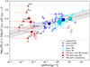 |
Fig. 3. Ratio of CO(5–4) to CO(2–1), a proxy for gas excitation, as a function of specific star formation rate. Our sample is shown with red circles (non mergers) and stars (mergers) and is compared to literature samples of local star-forming galaxies (blue pentagons), (U)LIRGs (blue squares), high-redshift main-sequence galaxies (cyan circles), and high-redshift SBs (cyan squares; Liu et al. 2021). The companions of ID83492 are shown as brown circles. For post-SBs without CO(2–1) observations, empty symbols indicate a pseudo CO(2–1) estimated from the CO(3–2) assuming the average local post-SBs R32 = 0.62 ratio (French et al. 2023). Large symbols indicate the population averages (see Sect. 4.1). A fit to the literature samples (solid gray line) with its scatter (shaded area) from Valentino et al. (2020) is shown and extrapolated toward lower sSFR (dashed gray line). |
We also include the two star-forming companions of ID83492, as well as comparison samples of local and high-redshift main-sequence galaxies, local Ultra Luminous Infrared Galaxies (ULIRGs), and high-redshift SBs from the literature (Liu et al. 2021). The post-SBs extend the region of parameter space sampled by star-forming galaxies toward lower sSFR. All our sample galaxies are detected in CO(2–1), while only 3 are detected in CO(5–4). Non-detections have on average a tight upper limit of R52 < 0.10 (1σ) derived by stacking (see Sect. 3.1). This is twice smaller than the average for local star-forming galaxies, and 2.6–3.7 times lower than the R52 of (U)LIRGs, high-redshift SBs and main-sequence galaxies. This suggests a reduced fraction of dense, warm gas relative to cold, diffuse molecular gas.
The three CO(5–4) detections in our sample instead have, on average, a higher R52 = 0.40, more comparable to that of high-redshift SBs, than the rest of the sample. We note that only the CO(5–4) detections in our sample correspond to mergers, while galaxies without detections show no evidence of companions or merger signatures (e.g., tidal tails). Their relatively high R52 ratio suggests that quenching is still ongoing in these systems, with star formation likely depleting the remaining molecular gas on short timescales. Such behavior indicates that gas exhaustion and potentially gas stripping are important mechanisms to keep galaxies quiescent. Interestingly, the two star-forming companions of ID83492 have sSFRs comparable to those of SB galaxies, but their R52 values are lower by about 0.5 dex and comparable to the most stringent upper limits in our sample. This suggests that the ongoing merger has affected the molecular gas properties of all the galaxies involved, and that a mismatch between the timescales traced by R52 and sSFR is key to interpreting these results (see Section 5).
Finally, we computed the average R52 ratio of the entire sample by employing the Kaplan–Meier estimator from survival analysis to properly account for both detections and upper limits4. We find and average R52 = 0.28 (Table 4). To estimate the associated uncertainties, we employed a bootstrap resampling approach.
Mean specific star formation and R52 ratio for our sample.
We also investigated if the R52 ratio correlates with other physical properties, such as the depth of the 4000 Å break (Dn4000 Å), the time since quenching (tq), or the molecular gas fraction (fH2). We do not find any clear correlation with Dn4000 Å or tq, and a mild trend with fH2 (Fig. B.1). However, a larger sample with more detections is needed to confirm it. In Table 4 we report the R52 of our sample.
4.2. Spectral line energy distribution
The CO SLED traces how the radiated energy is distributed among the different J transitions of the CO ladder and provides a powerful diagnostic of the physical conditions of the ISM. It has been shown that the CO SLED can distinguish between galaxies with low SFRs, such as the Milky Way, whose emission peaks at intermediate J = 3 − 4 (Weiß et al. 2005; Carilli & Walter 2013), and dense, warm SBs, whose emission peaks at higher J = 7 − 8 (Weiss et al. 2007; Vallini et al. 2019; Esposito et al. 2024). In the presence of active AGN, even higher excitation is observed due to the contribution of X-ray-dominated regions (van der Werf et al. 2010). Both observational (Papadopoulos et al. 2012; Daddi et al. 2015; Valentino et al. 2020; Liu et al. 2021) and theoretical studies (Narayanan & Krumholz 2014; Bournaud et al. 2015; Vollmer et al. 2017) have shown that high-redshift star-forming galaxies have higher molecular gas fractions, denser gas, and enhanced SFRs (Daddi et al. 2010; Genzel et al. 2010; Tacconi et al. 2018), resulting in SLEDs that peak at higher J = 4 − 5 compared to local star-forming galaxies.
By complementing our observations with archival CO(2–1), CO(3–2), and CO(4–3) data when available, we investigated the CO SLEDs of post-SBs and compared them with literature observational and theoretical results. In Figure 4, we show the individual SLEDs of our sample galaxies, all normalized to the CO(2–1) transition. As before, for the two galaxies lacking CO(2–1) observations, we derived a pseudo CO(2–1) using R32 = 0.50 (see Section 4.1). We find a diversity of SLED shapes among our post-SBs, with some peaking at J ≥ 5 (e.g., J1448, J2258) and others peaking at J = 3 (e.g., ID97148, J0912). The average SLED of our targets peaks at J = 4 and exhibits a shape comparable to the Milky Way SLED (Carilli & Walter 2013).
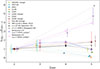 |
Fig. 4. CO SLED of our post-SB galaxies flux ratio. Individual galaxies are shown with small colored circles (measurements) and down-pointing triangles (3σ upper limits), while the average SLED is indicated by empty red circles. For comparison, we also show the Milky Way SLED (black squares; Carilli & Walter 2013), the average SLED of main-sequence galaxies (filled black triangles from Valentino et al. 2020 and empty black triangles from Boogaard et al. 2020), and the SLED predicted by the model of Narayanan & Krumholz (2014) assuming a SFR surface density of ΣSFR = 0.05 M⊙ yr−1 kpc−2 (blue diamonds) and ΣSFR = 500 M⊙ yr−1 kpc−2 (pink diamonds). |
The emission of two of the three confirmed mergers in our sample peaks at J ≥ 5, similar to what is observed in high-redshift main-sequence galaxies (Valentino et al. 2020; Boogaard et al. 2020). For the remaining merger, only two data points are available (CO(3–2) and CO(5–4)), so additional observations are required to fully constrain the shape of its SLED.
Finally, we compared our observations with the model proposed by Narayanan & Krumholz (2014), which links a galaxy’s mean SFR surface density (ΣSFR), a proxy for gas density and temperature, to the shape of its SLED. We show in Fig. 4 the SLED predicted for ΣSFR = 0.05 M⊙ yr−1 kpc−2, consistent with the average ΣSFR of our sample galaxies computed using their optical size. This model reproduces the shape of the average SLED of our post-SBs, peaking at J ∼ 4 and declining at higher J.
To reproduce the SLEDs of J1448 and J2258, higher ΣSFR values are required. In particular, models with ΣSFR ∼ 300 − 500 M⊙ yr−1 kpc−2 are needed to reproduce the rising SLED of J2258 up to J = 5, similar to high-redshift SBs, although additional data points at intermediate J (e.g., CO(3–2), CO(4–3)) are needed to fully constrain its shape. Instead even models with very high SFR surface densities (ΣSFR > 500 M⊙ yr−1 kpc−2) struggle to reproduce the SLED of J1448, which rises steeply toward higher J transitions. The extreme shape of this SLED could be due to the presence of an AGN and/or shocks (Narayanan & Krumholz 2014). Indeed, the optical spectrum of J1448 shows luminous and broad [OIII] and Hα emission lines, indicative of AGN activity (Greene et al. 2020; D’Onofrio et al. 2025; Zhu et al. 2025), and VLA 6 GHz observations reveal a morphology consistent with compact, young radio jets (D’Onofrio et al. 2025). Additionally, shocks from AGN outflows and/or the ongoing merger may further enhance the CO excitation.
For the other two mergers in our sample, evidence of AGN activity is less clear. In J2258, D’Onofrio et al. (2025) report only faint Hα emission and compact, weak radio emission consistent with past star formation. Optical and radio data for ID83492 are not available; however, it is covered by deep Chandra observations5, which also yielded no detection (Evans et al. 2024).
4.3. Residual star formation
Some works have found that a non-negligible fraction (∼25%) of local gas-rich post-SBs host obscured star formation at levels consistent with those observed in star-forming galaxies and SBs, thereby questioning their truly quiescent nature (Poggianti & Wu 2000; Smercina et al. 2018; Baron et al. 2022, 2023). Interestingly, our galaxy J1448, which exhibits a 60 kpc-long CO(2–1) tidal tail (Spilker et al. 2022) due to an ongoing merger, also shows pockets of star formation traced by Hα in the northern tail, as revealed by HST/WFC3 spectroscopy (D’Onofrio et al. 2025). One of these Hα-emitting regions also emits CO(5–4), indicating a dense molecular gas clump actively forming stars. Hα and [OIII] are also detected in the galaxy core; however, these are consistent with AGN activity (Zhu et al. 2025; D’Onofrio et al. 2025), suggesting that the core is transitioning toward quiescence. Faint Hα is reported in the core of J2202 as well, though it is unclear if it originates from residual star formation or AGN (D’Onofrio et al. 2025). Finally, ID83492 and ID97148 show [OII], which may arise from residual star formation (dust-corrected SFR = 0.2 M⊙ yr−1 for ID97148 and 0.3 M⊙ yr−1 for ID83492; Zanella et al. 2023) or AGN activity.
We used the CO(5–4) – LIR relation calibrated on star-forming galaxies as a consistency test to assess whether the CO(5–4) line luminosities observed in our sample could plausibly arise from obscured star formation. We converted the CO(5–4) luminosity into total IR luminosity (LIR) following the relation of Valentino et al. (2020), and then converted LIR into SFR using the relation from Kennicutt & De Los Reyes (2021). While undetected galaxies have relatively low SFRs (SFR ≲ 20 M⊙ yr−1), the three sources with detected CO(5–4) emission would imply significantly higher obscured SFRs (SFR ∼ 20 − 140 M⊙ yr−1). We verified whether such high IR luminosities are consistent with the non-detections in the dust continuum. To this end, we used the average SED template for quiescent galaxies from Magdis et al. (2021), which is characterized by a dust temperature Td = 20 K, and we rescaled it to match the most stringent dust continuum 3σ upper limit available for each galaxy. This yielded the maximum LIR allowed by the lack of continuum detection, and maximum obscured SFRs < 18 M⊙ yr−1, consistent with values expected for quiescent galaxies. However, Valentino et al. (2020) calibrated the CO(5–4) – LIR using templates typical of high-redshift star-forming galaxies, and hence with higher dust temperatures (Td). We repeated the calculation using a warmer SED template (Td = 30 K) obtained by scaling the Magdis et al. (2021) SED with a modified blackbody. This yielded even lower maximum LIR and more stringent SFR < 11 M⊙ yr−1.
In Figure 5 we compare the observed CO(5–4) luminosity with the maximum LIR allowed by the dust continuum non-detections. The majority of the measurements do not follow the CO(5–4) – LIR relation calibrated for star-forming galaxies (Valentino et al. 2020). For dust temperatures of 20 K, only one detected source and three non-detections are potentially consistent with the relation; for a warmer SED with Td = 30 K, this number further decreases. To place tighter constraints on the average properties of the two populations, we also derived stacked measurements separately for detections and non-detections. We find that the stack of the detected galaxies is inconsistent with the relation, while the stack of the non-detections remains potentially consistent. Deeper observations and larger samples are needed to assess whether non-detections lie on the relation or significantly deviate from it.
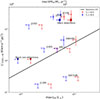 |
Fig. 5. CO(5–4) luminosity of our sample compared with the maximum IR luminosity allowed by the continuum non-detections. We computed the maximum LIR by considering the average SED template from Magdis et al. (2021) and rescaling it to match the observations. We considered both a template with dust temperature of 20 K (red circles) and 30 K (blue squares, see Sect. 4.3). We report both individual measurements (empty symbols) and stacking (filled diamonds for detections, down-pointing triangles for non-detections). We plot (black line) the CO(5–4) – LIR relation estimated by Valentino et al. (2020) for star-forming galaxies. The top axis indicates the SFR estimated from the maximum LIR with the Kennicutt & De Los Reyes (2021) conversion. |
The mismatch observed for most detections, and potentially also for the non-detections, indicates that the CO(5–4) – LIR relation does not apply to the majority of our sample. This result reinforces our conclusion from Sect. 4.2 that the CO(5–4) emission detected in post-SB galaxies is unlikely to be predominantly powered by ongoing star formation. Instead, in at least some systems, the emission is more plausibly driven by alternative excitation mechanisms, such as shocks associated with mergers and/or AGN-related processes. More generally, our results highlight that CO(5–4) – LIR scaling relations calibrated on star-forming galaxies must be applied with caution when interpreting quiescent or post-SB systems. This interpretation is consistent with recent findings suggesting that gas and dust in post-SB and quiescent galaxies are decoupled, exhibiting gas-to-dust ratios that are orders of magnitude higher than in star-forming galaxies (Spilker et al. 2025). We report all the LIR and SFR measurements in Table C.1.
5. Discussion
Our post-SB galaxies exhibit an average R52 ∼ 0.28 (from survival analysis) comparable to high-redshift star-forming galaxies. However, we find a significantly lower ratio (R52 < 0.10) when stacking only the galaxies that are not detected in CO(5–4) and do not show signs of interaction, a value twice lower than local star-forming galaxies and 2.5 times lower than high-redshift ones. This suggests a reduced fraction of dense and/or warm molecular gas relative to cold and diffuse gas in these sources, consistent with previous studies of local early-type (Crocker et al. 2012; Bayet et al. 2013) and post-SB galaxies (French et al. 2023).
As highlighted by French et al. (2023), the excitation of CO-traced molecular gas can help distinguish between different mechanisms responsible for the low SFE observed in post-SBs. Low SFE is thought to arise from a deficit of dense molecular gas; however, the excitation of the remaining gas depends on its kinetic temperature and density, and thus provides an insight into the underlying physical processes. Elevated kinetic temperatures, potentially driven by turbulence, shocks, or AGN activity, would result in high excitation, whereas low-density gas with modest temperatures would produce low excitation levels similar to those observed in early-type galaxies.
The average CO excitation of the post-SB galaxies in our sample favors this latter scenario, pointing to molecular gas that is predominantly diffuse, cold, and inefficient at forming stars. This interpretation is consistent with the low-excitation CO SLEDs observed in local post-SBs by French et al. (2023), who constrained transitions up to CO(3–2), and supports a picture in which quenching is maintained by a deficit of dense star-forming gas rather than by widespread heating alone. Such a low dense-gas fraction suggests that gas stabilization processes, such as morphological quenching (Martig et al. 2009; Johansson et al. 2009) or enhanced turbulence that prevents the collapse of gas into giant molecular clouds (Smercina et al. 2022), play a dominant role in suppressing star formation in these systems.
For the three post-SBs in our sample that are currently undergoing a merger, however, the physical conditions of the molecular gas may be different. Although their R52 values are comparable to those of main-sequence galaxies, this similarity does not necessarily imply a common excitation mechanism. In these systems, the elevated high-J CO emission may instead arise from enhanced heating, potentially driven by merger-induced shocks and/or AGN activity. Galaxy mergers are known to strongly perturb the interstellar medium, generating shocks and turbulence that can modify the gas density and temperature distribution. In particular, compressive turbulence during mergers can increase the fraction of dense gas (e.g., Barnes & Hernquist 1991; Jog & Solomon 1992; Renaud et al. 2014, 2022), especially during the first pericenter passages, in contrast to the predominantly solenoidal turbulence inferred in local post-SBs by Smercina et al. (2022) and French et al. (2023) that suppresses star formation while maintaining low CO excitation. High-resolution simulations by Bournaud et al. (2015) show that major mergers exhibit significantly more excited CO SLEDs than local spirals, with CO(5–4)/CO(1–0) intensity ratios on average a factor of ∼8 higher in starbursting mergers. This enhanced excitation is attributed to dense gas created by large-scale inflows and merger-driven turbulence on small scales. Observational studies of local mergers similarly report elevated CO excitation associated with warm and/or dense molecular gas, potentially linked to enhanced turbulence and cosmic-ray heating (Papadopoulos et al. 2012; Liu et al. 2021). We also notice that for the two sources in our sample (J1448 and J2258) with the highest excitation, the CO(5–4) emission has broader linewidth than the CO(2–1), further indicating that the kinematics of the warm gas phase might be perturbed by merger-driven turbulence, inflows, outflows, and/or shocks.
In at least one of the merging post-SBs in our sample, we also find evidence of AGN activity. Both X-ray irradiation from the AGN and shocks associated with outflows have been shown to enhance CO excitation (Vallini et al. 2019), and may contribute to the steeply rising SLED of J1448. High-resolution morphological and kinematic observations of the CO-emitting gas will be essential to determine the spatial origin of the dense and/or warm molecular component in these systems and to disentangle the respective roles of turbulence, mergers, and AGN feedback in maintaining quenching.
Interestingly, the companion galaxies of ID83492 show R52 values 0.5 dex lower than those of high-redshift SBs with comparable sSFRs. This likely reflects a mismatch in timescales: while sSFR traces star formation averaged over tens of Myr, CO(5–4) probes the instantaneous reservoir of dense and warm gas. In a merger-driven SB, the dense gas phase can be rapidly consumed or disrupted (e.g., Petersson et al. 2023), leading to low R52 even while the galaxy still appears star-forming. Future observations of Hα or Paα lines will help constrain the instantaneous SFR and assess whether a timescale mismatch indeed underlies the apparent tension between the R52 and sSFR in these systems. Additionally, observations of multiple CO transitions will be key to better constrain the SLEDs of these galaxies.
We note, however, that our analysis is limited to post-SBs with existing low-J CO detections, which may represent the gas-rich tail of the population. The processes responsible for shutting down star formation and those that subsequently maintain quiescence may therefore differ in gas-poor passive galaxies. Spatially resolved observations would provide stronger constraints by mapping the extent of both high-J and low-J CO emission and identifying potential spatial variations in excitation across the galaxies. In addition, higher-S/N data would enable dynamical studies to assess whether the molecular gas is gravitationally stable and to search for evidence of outflows.
None of the galaxies in our sample are detected in the dust continuum, despite the fact that, based on their CO(5–4) detections and the CO(5–4) – LIR relation from Valentino et al. (2020), we would have expected at least some detections. This result suggests that the CO(5–4) – LIR relation established for star-forming galaxies may not hold for quiescent systems, and that molecular gas and dust could be decoupled in passive galaxies. This interpretation is consistent with recent studies reporting unexpectedly weak dust emission and unusually high gas-to-dust ratios (δGDR ∼ 300–1200; Spilker et al. 2025). These findings imply that dust continuum emission is an unreliable tracer of molecular gas in quiescent galaxies and highlight the need for alternative cold-gas diagnostics (e.g., CO). Future mid-IR observations of post-SB and quiescent systems will provide further insights into their SEDs, constrain their dust properties, and potentially reveal residual obscured star formation or AGN activity.
6. Summary and conclusions
We investigated the molecular gas excitation of eight post-SB galaxies at z ∼ 0.6 − 1.3 by comparing CO(5–4) emission with archival CO(2–1), CO(3–2), and CO(4–3) data. To our knowledge, this is the first time that high-J CO transitions are probed for quiescent galaxies at these redshifts. All galaxies in our sample are detected in low-J CO transitions and have molecular gas fractions up to ∼30% (Bezanson et al. 2022; Zanella et al. 2023). Our main findings are as follows:
-
Three out of the eight galaxies are detected in CO(5–4). All three show signs of ongoing mergers or interactions, either in the form of tidal tails (J1448 and J2258; Spilker et al. 2022; D’Onofrio et al. 2025) or via two nearby star-forming companion galaxies (ID83492; Zanella et al. 2023).
-
We used the R52 = L′CO(5 − 4)/L′CO(2 − 1) ratio as a proxy for molecular gas excitation. On average, our post-SB galaxies have R52 = 0.28 (from survival analysis), comparable to high-redshift main-sequence galaxies. However, when considering only the non-detections (coinciding also with sources that do not show signs of interaction), we estimate a significantly lower R52 < 0.10 (from stacking), 2 times lower than local star-forming galaxies and > 2.5 times lower than high-redshift main-sequence and SB galaxies. In contrast, the three merging post-SBs exhibit higher R52 ∼ 0.49, more similar to high-redshift SBs. Interestingly, the two star-forming companions of ID83492, which have sSFRs comparable to SB galaxies, show R52 values ∼0.5 dex lower than typical main-sequence sources.
-
The CO SLEDs of our post-SBs are diverse, with an average peak at J = 3, similar to the Milky Way. The merging galaxies, however, have SLEDs peaking at higher J, more akin to high-redshift main-sequence galaxies, with J1448 being the most extreme case, likely requiring additional mechanisms (e.g., shocks or AGN activity) to explain its elevated excitation.
-
Residual obscured star formation cannot fully account for the CO(5–4) emission in the detected galaxies, because assuming the CO(5–4) – LIR relation for star-forming galaxies (Valentino et al. 2020) and the typical SED of quiescent galaxies (Magdis et al. 2021), they would have been detected in the dust continuum. Additionally, the fact that our post-SBs do not agree with the CO(5–4) – LIR relation and that none of them is detected in dust continuum indicates that molecular gas and dust in quiescent galaxies might be decoupled, as recently suggested by Spilker et al. (2025).
-
Our results indicate that, for the majority of our post-SBs, the molecular gas is predominantly diffuse and cold, leading to low CO excitation consistent with that observed in local post-SBs (French et al. 2023). This suggests that the suppression of star formation is primarily maintained by a low fraction of dense molecular gas, favoring quenching mechanisms such as gas stabilization or enhanced turbulence that prevent the gas from fragmenting and collapsing, rather than by widespread heating of the molecular medium. For the merging post-SBs, however, the higher CO excitation indicates elevated kinetic temperatures, likely induced by shocks and/or AGN activity, which act to suppress star formation.
Larger samples of high-redshift post-SBs with multi-transition CO observations will be essential to confirm and expand upon these results. Recently, Setton et al. (2025) published a sample of 50 post-SBs with CO(2–1) data that could in principle be followed-up with observations of higher J CO transitions. In particular, homogeneously observing multiple CO transitions across large samples will allow statistical constraints to be placed on the SLED and help determine whether elevated excitation is common in merging post-SBs. In addition, further investigating the SLED of passive galaxies might shed light on the αCO factor that needs to be used to convert low-J CO luminosities into molecular gas masses. Current works (e.g., French et al. 2015; French 2021; Suess et al. 2017; Bezanson et al. 2022; Zanella et al. 2023; Setton et al. 2025) typically adopt the Milky-Way conversion factor. However, αCO might depend on the SLED of the galaxy population and could therefore be different in quiescent galaxies. Higher-resolution observations will further enable measurements of the CO-emitting region’s size, morphology, and dynamics, and help deblend close galaxy pairs, clarifying whether mergers are ubiquitous in the post-SB population and their role in suppressing star formation. Finally, assessing the presence of AGNs and potential molecular outflows will be critical to understanding the contribution of AGN feedback and shocks to quenching.
Data availability
The data used in this study are available from telescope archives. Software and derived data generated for this research can be made available upon reasonable request to the corresponding author.
Acknowledgments
We thank the referee for the insightful report. AZ thanks F. Vito for useful discussions about the X-ray detection and AGN activity of our galaxies. SB is supported by ERC grant 101076080. FV acknowledges support from the Independent Research Fund Denmark under grant 3120-00043B and the Danish National Research Foundation under grant DNRF140. This paper makes use of the following ALMA data: 2016.1.01126.S; 2017.1.01109.S; 2018.1.01264.S; 2018.1.01240.S; 2019.1.00221.S; 2019.1.00900.S; 2024.1.00061.S. ALMA is a partnership of ESO (representing its member states), NSF (USA), and NINS (Japan), together with NRC (Canada), MOST and ASIAA (Taiwan), and KASI (Republic of Korea), in cooperation with the Republic of Chile. The Joint ALMA Observatory is operated by ESO, AUI/NRAO and NAOJ.
References
- Abolfathi, B., Aguado, D. S., Aguilar, G., et al. 2018, ApJS, 235, 42 [NASA ADS] [CrossRef] [Google Scholar]
- Barnes, J. E., & Hernquist, L. E. 1991, ApJ, 370, L65 [Google Scholar]
- Baron, D., Netzer, H., Lutz, D., Prochaska, J. X., & Davies, R. I. 2022, MNRAS, 509, 4457 [Google Scholar]
- Baron, D., Netzer, H., French, K. D., et al. 2023, MNRAS, 524, 2741 [NASA ADS] [CrossRef] [Google Scholar]
- Bayet, E., Bureau, M., Davis, T. A., et al. 2013, MNRAS, 432, 1742 [Google Scholar]
- Belli, S., Contursi, A., Genzel, R., et al. 2021, ApJ, 909, L11 [NASA ADS] [CrossRef] [Google Scholar]
- Bezanson, R., Spilker, J. S., Suess, K. A., et al. 2022, ApJ, 925, 153 [NASA ADS] [CrossRef] [Google Scholar]
- Bolatto, A. D., Wolfire, M., & Leroy, A. K. 2013, ARA&A, 51, 207 [CrossRef] [Google Scholar]
- Boogaard, L. A., van der Werf, P., Weiss, A., et al. 2020, ApJ, 902, 109 [NASA ADS] [CrossRef] [Google Scholar]
- Bournaud, F., Daddi, E., Weiß, A., et al. 2015, A&A, 575, A56 [NASA ADS] [CrossRef] [EDP Sciences] [Google Scholar]
- Bower, R. G., Benson, A. J., Malbon, R., et al. 2006, MNRAS, 370, 645 [Google Scholar]
- Bruzual, G., & Charlot, S. 2003, MNRAS, 344, 1000 [NASA ADS] [CrossRef] [Google Scholar]
- Calzetti, D., Armus, L., Bohlin, R. C., et al. 2000, ApJ, 533, 682 [NASA ADS] [CrossRef] [Google Scholar]
- Carilli, C. L., & Walter, F. 2013, ARA&A, 51, 105 [NASA ADS] [CrossRef] [Google Scholar]
- Chabrier, G. 2003, PASP, 115, 763 [Google Scholar]
- Combes, F. 2018, A&ARv, 26, 5 [NASA ADS] [CrossRef] [Google Scholar]
- Combes, F., Young, L. M., & Bureau, M. 2007, MNRAS, 377, 1795 [NASA ADS] [CrossRef] [Google Scholar]
- Couch, W. J., & Sharples, R. M. 1987, MNRAS, 229, 423 [NASA ADS] [CrossRef] [Google Scholar]
- Crocker, A., Krips, M., Bureau, M., et al. 2012, MNRAS, 421, 1298 [NASA ADS] [CrossRef] [Google Scholar]
- Croton, D. J., Springel, V., White, S. D. M., et al. 2006, MNRAS, 365, 11 [Google Scholar]
- Daddi, E., Bournaud, F., Walter, F., et al. 2010, ApJ, 713, 686 [NASA ADS] [CrossRef] [Google Scholar]
- Daddi, E., Dannerbauer, H., Liu, D., et al. 2015, A&A, 577, A46 [NASA ADS] [CrossRef] [EDP Sciences] [Google Scholar]
- Dannerbauer, H., Daddi, E., Riechers, D. A., et al. 2009, ApJ, 698, L178 [NASA ADS] [CrossRef] [Google Scholar]
- Davé, R., Rafieferantsoa, M. H., Thompson, R. J., & Hopkins, P. F. 2017, MNRAS, 467, 115 [NASA ADS] [Google Scholar]
- Dekel, A., & Birnboim, Y. 2006, MNRAS, 368, 2 [NASA ADS] [CrossRef] [Google Scholar]
- Dey, A., Schlegel, D. J., Lang, D., et al. 2019, AJ, 157, 168 [Google Scholar]
- Di Matteo, T., Springel, V., & Hernquist, L. 2005, Nature, 433, 604 [NASA ADS] [CrossRef] [Google Scholar]
- D’Onofrio, V. R., Spilker, J. S., Bezanson, R., et al. 2025, ApJ, 990, 166 [Google Scholar]
- Dressler, A., & Sandage, A. 1983, ApJ, 265, 664 [NASA ADS] [CrossRef] [Google Scholar]
- Duncan, K. J. 2022, MNRAS, 512, 3662 [NASA ADS] [CrossRef] [Google Scholar]
- Esposito, F., Vallini, L., Pozzi, F., et al. 2024, MNRAS, 527, 8727 [Google Scholar]
- Evans, I. N., Evans, J. D., Martínez-Galarza, J. R., et al. 2024, ApJS, 274, 22 [NASA ADS] [CrossRef] [Google Scholar]
- Feldmann, R., & Mayer, L. 2015, MNRAS, 446, 1939 [Google Scholar]
- Feldmann, R., Quataert, E., Hopkins, P. F., Faucher-Giguère, C.-A., & Kereš, D. 2017, MNRAS, 470, 1050 [NASA ADS] [CrossRef] [Google Scholar]
- French, K. D. 2021, PASP, 133, 072001 [NASA ADS] [CrossRef] [Google Scholar]
- French, K. D., Yang, Y., Zabludoff, A., et al. 2015, ApJ, 801, 1 [NASA ADS] [CrossRef] [Google Scholar]
- French, K. D., Yang, Y., Zabludoff, A. I., & Tremonti, C. A. 2018, ApJ, 862, 2 [NASA ADS] [CrossRef] [Google Scholar]
- French, K. D., Smercina, A., Rowlands, K., et al. 2023, ApJ, 942, 25 [NASA ADS] [CrossRef] [Google Scholar]
- Genzel, R., Tacconi, L. J., Gracia-Carpio, J., et al. 2010, MNRAS, 407, 2091 [NASA ADS] [CrossRef] [Google Scholar]
- Greene, J. E., Setton, D., Bezanson, R., et al. 2020, ApJ, 899, L9 [NASA ADS] [CrossRef] [Google Scholar]
- Guilloteau, S., & Lucas, R. 2000, ASP Conf. Ser., 217, 299 [Google Scholar]
- Gunn, J. E., Gott, J., & Richard, I. 1972, ApJ, 176, 1 [Google Scholar]
- Hatfield, P. W., Jarvis, M. J., Adams, N., et al. 2022, MNRAS, 513, 3719 [NASA ADS] [CrossRef] [Google Scholar]
- Hopkins, P. F., Somerville, R. S., Hernquist, L., et al. 2006, ApJ, 652, 864 [NASA ADS] [CrossRef] [Google Scholar]
- Jog, C. J., & Solomon, P. M. 1992, ApJ, 387, 152 [NASA ADS] [CrossRef] [Google Scholar]
- Johansson, P. H., Naab, T., & Ostriker, J. P. 2009, ApJ, 697, L38 [NASA ADS] [CrossRef] [Google Scholar]
- Kamenetzky, J., Privon, G. C., & Narayanan, D. 2018, ApJ, 859, 9 [Google Scholar]
- Kennicutt, R. C., Jr., & De Los Reyes, M. A. C. 2021, ApJ, 908, 61 [NASA ADS] [CrossRef] [Google Scholar]
- Khochfar, S., & Ostriker, J. P. 2008, ApJ, 680, 54 [Google Scholar]
- Khoperskov, S., Haywood, M., Di Matteo, P., Lehnert, M. D., & Combes, F. 2018, A&A, 609, A60 [NASA ADS] [CrossRef] [EDP Sciences] [Google Scholar]
- Kriek, M., & Conroy, C. 2013, ApJ, 775, L16 [NASA ADS] [CrossRef] [Google Scholar]
- Larson, R. B., Tinsley, B. M., & Caldwell, C. N. 1980, ApJ, 237, 692 [Google Scholar]
- Lawrence, A., Warren, S. J., Almaini, O., et al. 2007, MNRAS, 379, 1599 [Google Scholar]
- Leja, J., Johnson, B. D., Conroy, C., van Dokkum, P. G., & Byler, N. 2017, ApJ, 837, 170 [NASA ADS] [CrossRef] [Google Scholar]
- Leja, J., Carnall, A. C., Johnson, B. D., Conroy, C., & Speagle, J. S. 2019, ApJ, 876, 3 [Google Scholar]
- Liu, D., Daddi, E., Schinnerer, E., et al. 2021, ApJ, 909, 56 [NASA ADS] [CrossRef] [Google Scholar]
- Magdis, G. E., Gobat, R., Valentino, F., et al. 2021, A&A, 647, A33 [NASA ADS] [CrossRef] [EDP Sciences] [Google Scholar]
- Maltby, D. T., Almaini, O., Wild, V., et al. 2016, MNRAS, 459, L114 [NASA ADS] [CrossRef] [Google Scholar]
- Man, A., & Belli, S. 2018, Nat. Astron., 2, 695 [NASA ADS] [CrossRef] [Google Scholar]
- Martig, M., Bournaud, F., Teyssier, R., & Dekel, A. 2009, ApJ, 707, 250 [Google Scholar]
- McMullin, J. P., Waters, B., Schiebel, D., Young, W., & Golap, K. 2007, ASP Conf. Ser., 376, 127 [Google Scholar]
- Mehta, V., Scarlata, C., Capak, P., et al. 2018, ApJS, 235, 36 [NASA ADS] [CrossRef] [Google Scholar]
- Mihos, J. C., & Hernquist, L. 1996, ApJ, 464, 641 [Google Scholar]
- Narayanan, D., & Krumholz, M. R. 2014, MNRAS, 442, 1411 [NASA ADS] [CrossRef] [Google Scholar]
- Oke, J. B. 1974, ApJ, 189, L47 [NASA ADS] [CrossRef] [Google Scholar]
- Pacifici, C., Iyer, K. G., Mobasher, B., et al. 2023, ApJ, 944, 141 [NASA ADS] [CrossRef] [Google Scholar]
- Papadopoulos, P. P., van der Werf, P. P., Xilouris, E. M., et al. 2012, MNRAS, 426, 2601 [NASA ADS] [CrossRef] [Google Scholar]
- Peng, Y., Maiolino, R., & Cochrane, R. 2015, Nature, 521, 192 [Google Scholar]
- Petersson, J., Renaud, F., Agertz, O., Dekel, A., & Duc, P.-A. 2023, MNRAS, 518, 3261 [Google Scholar]
- Poggianti, B. M., & Wu, H. 2000, ApJ, 529, 157 [CrossRef] [Google Scholar]
- Popping, G., van Kampen, E., Decarli, R., et al. 2016, MNRAS, 461, 93 [NASA ADS] [CrossRef] [Google Scholar]
- Rees, M. J., & Ostriker, J. P. 1977, MNRAS, 179, 541 [NASA ADS] [CrossRef] [Google Scholar]
- Renaud, F., Bournaud, F., Kraljic, K., & Duc, P. A. 2014, MNRAS, 442, L33 [NASA ADS] [CrossRef] [Google Scholar]
- Renaud, F., Bournaud, F., Agertz, O., et al. 2019a, A&A, 625, A65 [NASA ADS] [CrossRef] [EDP Sciences] [Google Scholar]
- Renaud, F., Bournaud, F., Daddi, E., & Weiß, A. 2019b, A&A, 621, A104 [NASA ADS] [CrossRef] [EDP Sciences] [Google Scholar]
- Renaud, F., Segovia Otero, Á., & Agertz, O. 2022, MNRAS, 516, 4922 [NASA ADS] [CrossRef] [Google Scholar]
- Rowlands, K., Wild, V., Nesvadba, N., et al. 2015, MNRAS, 448, 258 [Google Scholar]
- Schreiber, C., Glazebrook, K., Nanayakkara, T., et al. 2018, A&A, 618, A85 [NASA ADS] [CrossRef] [EDP Sciences] [Google Scholar]
- Setton, D. J., Bezanson, R., Suess, K. A., et al. 2020, ApJ, 905, 79 [Google Scholar]
- Setton, D. J., Spilker, J. S., Bezanson, R., et al. 2025, AJ, 170, 351 [Google Scholar]
- Skelton, R. E., Whitaker, K. E., Momcheva, I. G., et al. 2014, ApJS, 214, 24 [Google Scholar]
- Smercina, A., Smith, J. D. T., Dale, D. A., et al. 2018, ApJ, 855, 51 [NASA ADS] [CrossRef] [Google Scholar]
- Smercina, A., Smith, J.-D. T., French, K. D., et al. 2022, ApJ, 929, 154 [NASA ADS] [CrossRef] [Google Scholar]
- Solomon, P. M., & Vanden Bout, P. A. 2005, ARA&A, 43, 677 [NASA ADS] [CrossRef] [Google Scholar]
- Spilker, J. S., Suess, K. A., Setton, D. J., et al. 2022, ApJ, 936, L11 [Google Scholar]
- Spilker, J. S., Whitaker, K. E., Narayanan, D., et al. 2025, ApJ, 993, L40 [Google Scholar]
- Springel, V., Di Matteo, T., & Hernquist, L. 2005, ApJ, 620, L79 [Google Scholar]
- Suess, K. A., Bezanson, R., Spilker, J. S., et al. 2017, ApJ, 846, L14 [NASA ADS] [CrossRef] [Google Scholar]
- Suess, K. A., Kriek, M., Price, S. H., & Barro, G. 2021, ApJ, 915, 87 [NASA ADS] [CrossRef] [Google Scholar]
- Suess, K. A., Kriek, M., Bezanson, R., et al. 2022, ApJ, 926, 89 [NASA ADS] [CrossRef] [Google Scholar]
- Suess, K. A., Beverage, A. G., Kriek, M., et al. 2025, ApJ, 993, 158 [Google Scholar]
- Tacconi, L. J., Genzel, R., Saintonge, A., et al. 2018, ApJ, 853, 179 [Google Scholar]
- Valentino, F., Daddi, E., Puglisi, A., et al. 2020, A&A, 641, A155 [NASA ADS] [CrossRef] [EDP Sciences] [Google Scholar]
- Vallini, L., Tielens, A. G. G. M., Pallottini, A., et al. 2019, MNRAS, 490, 4502 [CrossRef] [Google Scholar]
- van der Werf, P. P., Isaak, K. G., Meijerink, R., et al. 2010, A&A, 518, L42 [NASA ADS] [CrossRef] [EDP Sciences] [Google Scholar]
- Vollmer, B., Gratier, P., Braine, J., & Bot, C. 2017, A&A, 602, A51 [NASA ADS] [CrossRef] [EDP Sciences] [Google Scholar]
- Weiß, A., Walter, F., & Scoville, N. Z. 2005, A&A, 438, 533 [NASA ADS] [CrossRef] [EDP Sciences] [Google Scholar]
- Weiss, A., Downes, D., Walter, F., & Henkel, C. 2007, ASP Conf. Ser., 375, 25 [NASA ADS] [Google Scholar]
- Wellons, S., Torrey, P., Ma, C.-P., et al. 2015, MNRAS, 449, 361 [Google Scholar]
- Werle, A., Poggianti, B., Moretti, A., et al. 2022, ApJ, 930, 43 [NASA ADS] [CrossRef] [Google Scholar]
- Wild, V., Almaini, O., Dunlop, J., et al. 2016, MNRAS, 463, 832 [NASA ADS] [CrossRef] [Google Scholar]
- Young, J. S., & Scoville, N. Z. 1991, ARA&A, 29, 581 [Google Scholar]
- Young, L. M., Bureau, M., Davis, T. A., et al. 2011, MNRAS, 414, 940 [NASA ADS] [CrossRef] [Google Scholar]
- Zanella, A., Valentino, F., Gallazzi, A., et al. 2023, MNRAS, 524, 923 [CrossRef] [Google Scholar]
- Zhu, P., Suess, K. A., Kriek, M., et al. 2025, ApJ, 981, 60 [Google Scholar]
- Zolotov, A., Dekel, A., Mandelker, N., et al. 2015, MNRAS, 450, 2327 [Google Scholar]
We performed the entire analysis, including flux measurements, in the uv plane. Being based on the raw interferometric visibilities, it does not require image reconstruction or deconvolution, avoiding biases and artefacts introduced during imaging and cleaning, and allowing us to fully account for the spatial frequencies sampled by the array, as well as the instrumental resolution and sensitivity.
They also fit the spectra and photometry with delayed exponential SFHs Setton et al. (2020) assuming similar Chabrier (2003) IMF, Bruzual & Charlot (2003) libraries, and a Calzetti et al. (2000) dust law using FAST++. The stellar masses derived from these fits are an average of 0.38 dex lower than the stellar masses derived in the default fits.
We used the python package lifelines and the task KaplanMeierFitter.
Among our sources, only ID83492 and ID97148 are covered by deep Chandra observations, which did not detect them (Evans et al. 2024).
Appendix A: Continuum detections
We searched for dust continuum detections nearby our targets and found several targets. We detected the following sources:
-
four galaxies with a projected distance of 6.0″ − 15.3″ ∼ 50.5 − 129.6 kpc from ID83492. All of them are detected in HST/F160W optical imaging. The dust continuum detection of two of them, the brightest, was already reported by Zanella et al. (2023). They are also detected in CO(2–1) and CO(3–2) at a similar redshift as our main target. The remaining two do not show any emission lines in ALMA data. They have photometric redshifts from 3D HST (Skelton et al. 2014) of zphot = 1.9808 and zphot = 2.0229; hence they are likely at higher redshift than our target.
-
one galaxy at 9.7″ ∼ 83.4 kpc from ID97148 (5.4σ). This source is detected in optical VIRCAM H band data and it has several photometric redshift estimates from the literature in the range zphot = 2.0 − 2.4 (Mehta et al. 2018; Hatfield et al. 2022), indicating that this is likely a higher redshift source than our target.
-
one galaxy at 5.4″ ∼ 36.8 kpc from J1302 (5.4σ). The available photometric redshift estimate from the DESI survey zphot = 0.78 (Duncan 2022) indicates that this is likely a lower redshift galaxy than J1302.
We report in Table A.1 their coordinates and fluxes.
Coordinates and continuum flux of the sources serendipitously detected nearby our targets.
Appendix B: Molecular gas excitation
We investigated possible correlations between the CO(5–4)/CO(2–1) luminosity ratio and several galaxy properties, namely the 4000 Å break strength (Dn4000), the quenching timescale (tq), and the molecular gas fraction (MH2/M★), as shown in Fig. B.1. To quantify any trends, we computed both the Pearson and Spearman correlation coefficients. We found no statistically significant correlations for Dn4000, rP = 0.31 (p = 0.46) and for tq, rP = −0.32 (p = 0.54). The corresponding Spearman coefficients are similarly low (|rS|< 0.49) with p > 0.32. The only marginally significant correlation iw with MH2/M★, which gives Pearson coefficients rP = −0.64 (p = 0.0.9) and Spearman coefficients rS = −0.79) with p = 0.02. These results indicate that, within the current uncertainties and limited sample size, there is no compelling evidence of a correlation between the CO excitation (as traced by R52) and stellar population age or quenching timescale, and a marginal correlation with the gas content. The latter is to be explored with future datasets.
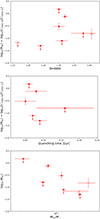 |
Fig. B.1. Molecular gas excitation traced by the CO(5-4)/CO(2-1) brightness temperature ratio (R52) as a function of galaxy properties. Top left: R52 versus the 4000Å break. Top right: R52 versus the time since quenching. Bottom: R52 versus the molecular gas fraction. |
Appendix C: Residual obscured star formation
We investigated whether our sample galaxies had residual star formation by converting the CO(5-4) luminosity into total IR luminosity following the relation of Valentino et al. (2020). We then converted the LIR into SFR by using the Kennicutt & De Los Reyes (2021) relation (see Section 4.3 for details). We also computed the maximum LIR consistent with the dust continuum non-detection considering the average SED template for quiescent galaxies from Magdis et al. (2021) both with a dust temperature of 20 K and 30 K. In Table C.1 we report the LIR and SFR obtained with the different methods.
IR luminosities and star formation rates.
All Tables
Coordinates and continuum flux of the sources serendipitously detected nearby our targets.
All Figures
|
Fig. 1. ALMA data of our galaxies. First column: 2D maps of the CO(5–4) line. The solid and dashed cyan contours indicate, respectively, positive and negative levels of (2.5, 3.5, 4.5, 5.5) rms. The beam is reported in the bottom left corner (white ellipse). Each stamp has a size of 10″ × 10″. The cyan cross indicates the center of our post-SBs as estimated from the optical emission. Second column: 1D spectra of sources extracted using a PSF to maximize the signal-to-noise ratio (S/N). The shaded pink areas indicate the 1σ velocity range over which we measured the CO(5–4) line flux or its upper limit. For detections we also report the Gaussian fit of the emissions (Sect. 3.1). The vertical dashed lines indicate the observed frequency corresponding to the redshift of the low-J CO emission. Third column: Rest-frame optical grz images from the DESI Legacy Survey DR9 Dey et al. (2019). The cyan contours show the CO(5–4) emission, while the orange and pink indicate the low-J (CO(2–1) or CO(3–2)) or CO(4–3) emission, respectively. The ellipses indicate the beam size. Each stamp has a size of 20″ × 20″. The contour levels are the same as in the first panels. (Continues on page 6). |
| In the text | |
|
Fig. 2. ALMA data of our galaxies (continued). As reported in Bezanson et al. (2022), the ∼1″ offset of the CO(2–1) of J2202 from the optical centroid is not significant given the data resolution and S/N. However, we note that the optical image of this galaxy appears to be slightly asymmetric. |
| In the text | |
|
Fig. 3. Ratio of CO(5–4) to CO(2–1), a proxy for gas excitation, as a function of specific star formation rate. Our sample is shown with red circles (non mergers) and stars (mergers) and is compared to literature samples of local star-forming galaxies (blue pentagons), (U)LIRGs (blue squares), high-redshift main-sequence galaxies (cyan circles), and high-redshift SBs (cyan squares; Liu et al. 2021). The companions of ID83492 are shown as brown circles. For post-SBs without CO(2–1) observations, empty symbols indicate a pseudo CO(2–1) estimated from the CO(3–2) assuming the average local post-SBs R32 = 0.62 ratio (French et al. 2023). Large symbols indicate the population averages (see Sect. 4.1). A fit to the literature samples (solid gray line) with its scatter (shaded area) from Valentino et al. (2020) is shown and extrapolated toward lower sSFR (dashed gray line). |
| In the text | |
|
Fig. 4. CO SLED of our post-SB galaxies flux ratio. Individual galaxies are shown with small colored circles (measurements) and down-pointing triangles (3σ upper limits), while the average SLED is indicated by empty red circles. For comparison, we also show the Milky Way SLED (black squares; Carilli & Walter 2013), the average SLED of main-sequence galaxies (filled black triangles from Valentino et al. 2020 and empty black triangles from Boogaard et al. 2020), and the SLED predicted by the model of Narayanan & Krumholz (2014) assuming a SFR surface density of ΣSFR = 0.05 M⊙ yr−1 kpc−2 (blue diamonds) and ΣSFR = 500 M⊙ yr−1 kpc−2 (pink diamonds). |
| In the text | |
|
Fig. 5. CO(5–4) luminosity of our sample compared with the maximum IR luminosity allowed by the continuum non-detections. We computed the maximum LIR by considering the average SED template from Magdis et al. (2021) and rescaling it to match the observations. We considered both a template with dust temperature of 20 K (red circles) and 30 K (blue squares, see Sect. 4.3). We report both individual measurements (empty symbols) and stacking (filled diamonds for detections, down-pointing triangles for non-detections). We plot (black line) the CO(5–4) – LIR relation estimated by Valentino et al. (2020) for star-forming galaxies. The top axis indicates the SFR estimated from the maximum LIR with the Kennicutt & De Los Reyes (2021) conversion. |
| In the text | |
|
Fig. B.1. Molecular gas excitation traced by the CO(5-4)/CO(2-1) brightness temperature ratio (R52) as a function of galaxy properties. Top left: R52 versus the 4000Å break. Top right: R52 versus the time since quenching. Bottom: R52 versus the molecular gas fraction. |
| In the text | |
Current usage metrics show cumulative count of Article Views (full-text article views including HTML views, PDF and ePub downloads, according to the available data) and Abstracts Views on Vision4Press platform.
Data correspond to usage on the plateform after 2015. The current usage metrics is available 48-96 hours after online publication and is updated daily on week days.
Initial download of the metrics may take a while.