| Issue |
A&A
Volume 709, May 2026
|
|
|---|---|---|
| Article Number | A49 | |
| Number of page(s) | 17 | |
| Section | Stellar structure and evolution | |
| DOI | https://doi.org/10.1051/0004-6361/202558219 | |
| Published online | 01 May 2026 | |
Competition between gravity waves excited by convection and tides in stars that host a companion
1
Instituut voor Sterrenkunde, KU Leuven, Celestijnenlaan 200D, 3001 Leuven, Belgium
2
CEA, DAM, DIF, F-91297 Arpajon, France
3
Observatoire de Genève, Université de Genève, Chemin Pegasi 51, 1290 Sauverny, Switzerland
4
Université Paris-Saclay, Université Paris Cité, CEA, CNRS, AIM, 91191 Gif-sur-Yvette, France
★ Corresponding author: This email address is being protected from spambots. You need JavaScript enabled to view it.
Received:
22
November
2025
Accepted:
27
March
2026
Abstract
Context. Asteroseismology has become a powerful diagnostic tool in stellar astrophysics, offering unprecedented insights into the internal structures and dynamics of stars. Through the analysis of stellar oscillation modes, it enables the precise characterisation of stellar interiors across a wide range of stellar masses and evolutionary phases, from the main sequence to the white dwarf phase. At the same time, the number of close stellar and planetary companions discovered throughout all stellar evolutionary phases has increased significantly, raising key questions about the interplay between stellar evolution and binarity.
Aims. In this study we investigated the competition between gravity waves excited by internal convection and those excited by tides in stars that host a companion. By modelling the energy and angular momentum luminosities transported by internal gravity waves stochastically excited by convection and by tides, we sought to quantify their relative contributions and identify the main parameters that govern their efficiency.
Methods. We computed the energy and angular momentum luminosities transported by both types of waves for a range of stellar masses and evolutionary stages, with a particular focus on understanding how the presence of a companion influences the angular momentum transport and the induced rotational evolution of the radiative layers of the host star.
Results. The competition between the two excitation mechanisms is sensitive to the mass and orbital properties of the companion, as well as the internal structure of the host star. We find that for a Jupiter-mass companion, the stochastic excitation dominates over tidal excitation during all evolutionary phases. Only for close-in stellar companions around late-type stars does the tidal excitation become more efficient.
Conclusions. The presence of a companion is unlikely to significantly alter the internal angular momentum transport in the radiative layers of the host star, simplifying the modelling of angular momentum transport driven by internal gravity waves in stars that host a companion.
Key words: waves / methods: numerical / planet-star interactions / binaries: close / stars: evolution / planetary systems
© The Authors 2026
 Open Access article, published by EDP Sciences, under the terms of the Creative Commons Attribution License (https://creativecommons.org/licenses/by/4.0), which permits unrestricted use, distribution, and reproduction in any medium, provided the original work is properly cited.
This article is published in open access under the Subscribe to Open model. This email address is being protected from spambots. You need JavaScript enabled to view it. to support open access publication.
1. Introduction
Asteroseismology has emerged as one of the most powerful diagnostic tools in stellar astrophysics, offering unprecedented insights into the internal structure and dynamics of stars. By analysing stellar oscillation modes, it is possible to probe the otherwise inaccessible interior of stars and to constrain key processes such as rotation, mixing, and energy transport. Over the past two decades, asteroseismology has transformed our understanding of stellar evolution across a wide range of masses and evolutionary phases, from main-sequence (MS) stars to compact remnants such as white dwarfs (WDs; Aerts et al. 2010; García & Ballot 2019; Christensen-Dalsgaard 2021; Aerts et al. 2021; Bowman & Bugnet 2026).
The advent of high-precision, long-duration space-based photometry from missions such as CoRoT (Baglin et al. 2006), Kepler (Borucki et al. 2010), and TESS (Ricker et al. 2015) has been especially transformative. These facilities have enabled the direct measurement of internal rotation at different points inside the star, revealing a consistent pattern of strong angular momentum redistribution from the stellar core to the envelope (Beck et al. 2012; Mosser et al. 2012; Deheuvels et al. 2012, 2014; Van Reeth et al. 2016; Gehan et al. 2018; Li et al. 2020; Aerts et al. 2025). Remarkably, the efficiency of this redistribution appears to be up to two orders of magnitude stronger than predicted by stellar evolution models that take into account a radial shellular differential rotation (Zahn 1992) and the related large-scale meridional circulation and hydrodynamical turbulence (Eggenberger et al. 2012; Ceillier et al. 2013; Marques et al. 2013; Cantiello et al. 2014; Ouazzani et al. 2019; Aerts et al. 2019). This discrepancy highlights a critical gap in our theoretical framework and has motivated intensive efforts to identify the physical mechanisms capable of transporting angular momentum with the required efficiency.
Of the proposed candidates, the two main mechanisms are magnetic fields and internal gravity waves (IGWs). The winding-up of weak magnetic fields by differential rotation can generate strong toroidal fields, the instabilities of which can drive (e.g. Tayler 1973) a Tayler-Spruit dynamo (Spruit 2002). This can lead to efficient angular momentum transport via the magnetic stresses (Petitdemange et al. 2023; Barrère et al. 2026) invoked to explain the nearly uniform rotation of the solar radiative interior (Eggenberger et al. 2005, 2022a) and the core rotation rates of evolved low-mass stars (Fuller et al. 2019; Eggenberger et al. 2022b). IGWs are excited at convective–radiative interfaces by turbulent motions in the convective regions of stars (Press 1981; Goldreich & Kumar 1990; Schatzman 1993; Belkacem et al. 2009; Lecoanet & Quataert 2013; Pinçon et al. 2016) and can efficiently mix chemical species and transport angular momentum in the radiative interior. Early pioneering work on the role of IGWs in stellar evolution dates back to Press (1981), Garcia Lopez & Spruit (1991), Schatzman (1993), and Zahn et al. (1997). These studies demonstrated that IGWs can play a crucial role in shaping stellar rotation profiles. More recently, IGWs have been invoked to explain the nearly uniform internal rotation of the Sun (Charbonnel & Talon 2005) and solar-type stars (Talon & Charbonnel 2005). Their influence has also been further explored in more massive stars (Rogers et al. 2013; Rogers 2015), as well as evolving subgiants (Fuller et al. 2014; Pinçon et al. 2017).
At the same time, observational surveys have revealed an ever-growing number of close stellar and planetary companions across virtually all evolutionary phases (e.g. Sana et al. 2012; Mulders et al. 2018; Beck et al. 2022; Hinkel et al. 2024; Esseldeurs et al. 2026). These discoveries have raised fundamental questions about the interplay between stellar evolution and binarity, for instance regarding the impact of companions on the internal and rotational evolution of their hosts (e.g. Mathis 2018; Ahuir et al. 2021b). One of the primary pathways through which a companion can alter the evolution of its host is via tides (Zahn 1994; Song et al. 2016). The gravitational interaction between the two bodies generates an ellipsoidal deformation of the host star, commonly referred to as the tidal bulge. The dissipation of this bulge in the convective envelope through turbulent viscosity gives rise to the so-called equilibrium tide (Zahn 1966, 1989; Remus et al. 2012), while the excitation of waves (e.g. IGWs at the convective–radiative interface) constitutes the dynamical tide.
Theoretical investigations of tidally excited IGWs date back to the seminal works of Zahn (1975, 1977) and Goldreich & Nicholson (1989), who first outlined the physical framework for tidal IGW dissipation in stars. Since then, the problem has been further developed in the context of wave excitation, propagation, and dissipation (e.g. Ogilvie & Lin 2004, 2007; Mathis 2015; Barker 2020; Ahuir et al. 2021a; Esseldeurs et al. 2024). While much of this work has focused on their role in tidal rotational and orbital evolution, tidally excited IGWs are also carriers of energy and angular momentum within the star (Goldreich & Nicholson 1989; Talon & Kumar 1998). This raises an intriguing question: to what extent do tidally induced gravity waves compete with, or even dominate over, the stochastic IGWs generated by convection?
In this study we investigated the competition between these two wave excitation mechanisms: stochastic excitation by convection and tidal excitation by a companion in stars across different evolutionary stages. Specifically, we modelled the associated energy and angular momentum luminosities and quantified their relative contributions under varying stellar and orbital conditions. We analysed a range of host star masses and evolutionary phases, with particular emphasis on how the presence of a close companion modifies the angular momentum transport of the host. We explored both stellar and planetary companions, examining how their masses and orbital separations influence the transport processes. In addition, we investigated the role of the host star’s internal structure and its evolution in regulating the efficiency of these processes.
In Sect. 2 we describe the theoretical framework used to model the energy and angular momentum transport by IGWs. In Sect. 3 we analyse the competition between convective and tidal excitation mechanisms, focusing on the dependence of their relative importance on key stellar and orbital parameters. In Sect. 4 we discuss the broader implications of our results for stellar rotation. Finally, a summary and conclusions are presented in Sect. 5.
2. Energy and angular momentum luminosities
2.1. Gravity waves in stars
Gravity waves (g-waves) are oscillations in a star that are restored by buoyancy. In stars, they propagate in stably stratified radiative zones, with frequencies lower than the Brunt-Väisälä frequency N (in rad/s) given by (Aerts et al. 2010)
 (1)
(1)
where g0, p0, and ρ0 are the unperturbed gravitational acceleration (in cm/s2), pressure (in g/cm s2), and density (in g/cm3), respectively. Γ1 = (∂lnp0/∂lnρ0)S is the first adiabatic exponent, where S is the macroscopic entropy.
In stars, gravity waves can be excited by various processes. To become excited, they need a source of energy, which can be provided at the interface between the convective and radiative layers. This energy can be provided by stochastic processes, such as turbulent convection, or by tidal interactions with a companion. The computation of the energy and angular momentum luminosities of these processes will be described in the following sections.
Once excited, gravity waves can propagate through the star. When propagating through the radiative zone, they can be dissipated by radiative damping. If this process is sufficiently strong, the waves will be dissipated before they reach the end of the radiative zone (a convective zone, the centre of the star, or the surface of the star). This is the regime of progressive waves. If the damping is weak, the waves will be able to propagate to the end of the radiative zone and reflect back inwards. In this case, the waves create standing modes. The transition between these two regimes is characterised by the critical frequency, ωcrit, separating g-modes and progressive gravity waves regimes. ωcrit (in rad/s) is given by (Alvan et al. 2015)
![Mathematical equation: $$ \begin{aligned} \omega _{\rm crit} = {[l(l+1)]}^{\frac{3}{8}}{\left(\left| \int _{r_{\rm in}}^{r_{\rm out}} K_{\mathrm{T} } \frac{N^3}{r_1^3}\ \mathrm{d} r_1\right|\right)}^{\frac{1}{4}}, \end{aligned} $$](/articles/aa/full_html/2026/05/aa58219-25/aa58219-25-eq2.gif) (2)
(2)
where KT is the thermal diffusivity (in cm2/s), rin and rout are the inner and outer radii of the radiative zone, respectively, and l is the spherical harmonic degree of the wave. In this work we only considered the case of progressive waves. Hence, we only considered the case where the waves are excited with a frequency below the critical frequency. This is the most suitable regime for angular momentum transport, as low-frequency IGWs are the most efficiently damped, which is necessary for angular momentum to be transported (e.g. Schatzman 1993; Zahn et al. 1997).
2.2. Stochastic excitation of gravity waves
The stochastic excitation of gravity waves is a process that occurs in stars with a radiative-convective interface (both from a convective core and a convective envelope envelope). At this interface, turbulent motions can generate gravity waves that propagate into the radiative zone. An order of magnitude of the energy flux of these waves can be computed based on the local properties of the star at this interface as in Press (1981, see also Lecoanet & Quataert 2013):
 (3)
(3)
where S stands for stochastic, ρint is the density and vc, int the convective velocity at the radiative-convective interface, ωc the angular frequency of the wave (the convective frequency in this case) and Nint the Brunt-Väisälä frequency at the location where the waves are excited. This flux can be integrated over the entire interface (in this case a spherical interface of radius rint) to obtain the energy luminosity:
 (4)
(4)
where ωc/Nint represents the Froude number. As this quantity is not always trivial to compute, it has been approximated to be roughly equal to the Mach number at the radiative-convective interface (see e.g. Fuller et al. 2014). For this reason the Froude number is sometimes called the convective Mach number in the literature. Another approach is to evaluate Nint directly at the radiative-convective interface. The comparison in Fig. C.1 shows that the two approaches lead to different results for the energy and angular momentum luminosities carried by stochastically excited waves by up to two orders of magnitude. However, the comparison of the angular momentum luminosities from the two approaches with the angular momentum luminosity of tidally excited waves remains robust because of their strong dependance on the orbital separation (see Fig. C.2).
To compute the Brunt-Väisälä frequency at the location where the waves are excited, we linearly expanded the (squared) Brunt-Väisälä frequency starting from the interface where this frequency is zero. We thus only considered the first-order term:
 (5)
(5)
where λ is a characteristic length scale of the variation in the gravity wave in the radial direction, defined as in Goodman & Dickson (1998) and Ahuir et al. (2021a):
 (6)
(6)
Therefore, we obtained the Brunt-Väisälä frequency at the location where the waves are excited as
 (7)
(7)
This allows us to rewrite the energy luminosity:
 (8)
(8)
In this case, ωc is the angular frequency of the convection, and thus ωc = 2π/tc, with tc = lc/vc the convective turnover time, computed at rint. This finally results in
 (9)
(9)
When calculating the angular momentum luminosity (LLS), this becomes
 (10)
(10)
The absolute value of LL gives the global torque applied on the studied radiative zone as progressive gravity waves are damped before reaching its other boundary (we refer the reader to Appendix E in Ahuir et al. 2021a).
In practice when computing these luminosities, the convective properties (vc, int and tc, int) and the change in the Brunt-Väisälä frequency (dN2/dlnr) are evaluated at the radiative-convective interface where the waves are launched. Here the mean of the properties through the first 30 data points inside the convective zone (for vc, int and tc, int) and inside the radiative zone (for dN2/dlnr) is used for more stable values for these properties. For interpretation purposes, it is useful to rewrite the convective velocity using the approximate formulation from mixing length theory (MLT) vc3 = L★/(ρCZR★2), with L★ the luminosity of the star, ρCZ the mean density in the convective zone, and R★ the radius of the star (Brun et al. 2017).
This expression for the angular momentum luminosity strongly relies on the monochromatic model from Press (1981) where it is assumed that convection excites gravity waves efficiently for ω ≈ ωc. It has been later refined with taking into account the possibility to excite a frequency spectrum (Garcia Lopez & Spruit 1991; Zahn et al. 1997), the contribution of the Reynolds stresses in the bulk of stellar convective regions (Goldreich & Kumar 1990; Belkacem et al. 2009), the nature of the stratification gradient at the radiative/convective interface (Lecoanet & Quataert 2013), and convective plumes (Schatzman 1993; Pinçon et al. 2016). The obtained predictions always scale with the vertical flux of kinetic energy carried by convection and the Froude number at the convective–radiative interface as proposed by Press (1981). At the same time, strong efforts have been done to develop and compute local and global hydrodynamical non-linear simulations of IGWs excitation by turbulent convection in stellar interiors (Rogers et al. 2013; Alvan et al. 2014; Couston et al. 2018; Edelmann et al. 2019; Le Saux et al. 2022; Breton et al. 2022; Anders et al. 2023; Herwig et al. 2023; Daniel & Lecoanet 2026). Although these simulations provide a more realistic description of the excitation process, they have confirmed that theoretical models, including the model proposed by Press (1981), provide a reasonable order-of-magnitude estimate of the total wave flux (Rogers et al. 2013; Alvan et al. 2014; Couston et al. 2018; Edelmann et al. 2019; Daniel & Lecoanet 2026).
Additionally, rotation itself can have an impact on the stochastic excitation of gravity waves through the formation of gravito-inertial waves (e.g. Augustson et al. 2020), or even magneto-gravito-inertial waves when magnetic fields are present (e.g. Mathis 2009; Mathis & de Brye 2012; Bessila & Mathis 2024). However, modelling (magneto-)gravito-inertial waves is out of scope for this work, and we refer the reader to Sect. 4 for a detailed discussion on the required developments. We relied on the simpler model from Press (1981) in the remainder of this work as a first estimate.
2.3. Tidal excitation of gravity waves
Tidal forces from a companion can excite gravity waves at the radiative-convective interface that propagate into the radiative zone. The tidal perturbation can be described by the tidal potential (Ogilvie 2014):
![Mathematical equation: $$ \begin{aligned} \begin{aligned} \Psi (r, \theta , \varphi , t) = \mathrm{Re} \Bigg [\sum _{l=2}^{\infty } \sum _{m=0}^l \sum _{n=-\infty }^{\infty }\Bigg \{\frac{G M_2}{a}&A_{l, m, n} (e, i)\left(\frac{r}{a}\right)^l\\&\times Y_l^m(\theta , \varphi ) \mathrm{e}^{-\mathrm{i} n \Omega _o t}\Bigg \}\Bigg ], \end{aligned} \end{aligned} $$](/articles/aa/full_html/2026/05/aa58219-25/aa58219-25-eq11.gif) (11)
(11)
where G is the gravitational constant, M2 the mass of the companion, a the semi-major axis of the orbit, Al, m, n(e, i) a coefficient that depends on the eccentricity (e) and inclination (i) of the orbit relative to the stellar spin, Ylm(θ, φ) the spherical harmonic function with degree l and order m, Ωo the orbital frequency, and ωt = nΩo − mΩs the tidal frequency in the frame rotating with the star, with Ωs the rotation frequency of the star. In this work we only considered circular (e = 0) and coplanar (i = 0) orbits, and thus only considered the dominant quadrupolar term (l = m = 2) with n = 2; this resulted in the following tidal potential:
 (12)
(12)
This tidal potential can excite gravity waves at the radiative-convective interface, which then propagate through the radiative zone. The energy and angular momentum luminosities of these waves has been computed by Ahuir et al. (2021a):
 (13)
(13)
 (14)
(14)
where Γ is the gamma function, and ℱ is the tidal forcing defined for both a convective core and a convective envelope (see Fig. 1 for a schematic representation of a three-layer stellar structure):
![Mathematical equation: $$ \begin{aligned} \begin{aligned} \mathcal{F} _{\mathrm{in} }&=\int _0^{r_{\rm in}} \left[{\left(\frac{r^2 \varphi _T}{g_0}\right)}^{\prime \prime } -\frac{l(l+1)}{r^2}\left(\frac{r^2 \varphi _T}{g_0}\right)\right] \frac{X_{1, \mathrm{in}}}{X_{1, \mathrm{in}}(r_{\mathrm{in} })} \mathrm{d} r \\ \mathcal{F} _{\mathrm{out} }&=\int _{r_{\mathrm{out} }}^{R_{\star }}\left[{\left(\frac{r^2 \varphi _T}{g_0}\right)}^{\prime \prime }-\frac{l(l+1)}{r^2}\left(\frac{r^2 \varphi _T}{g_0}\right)\right] \frac{X_{1, \mathrm{out}}}{X_{1, \mathrm{out}}(r_{\mathrm{out} })} \mathrm{d} r \end{aligned}, \end{aligned} $$](/articles/aa/full_html/2026/05/aa58219-25/aa58219-25-eq15.gif) (15)
(15)
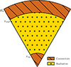 |
Fig. 1. Schematic view of the radiative and convective shells in the three-layer model used in this work. Radii are not to scale (see the Kippenhahn diagrams, e.g. Fig. 2). |
where rin and rout are the inner and outer boundaries of the radiative zone, respectively, and X1, out and X1, in are representations for the radial displacement originating from the inner and outer boundary of the radiative zone. The radial displacement can be calculated using the following differential equations and boundary conditions (Ahuir et al. 2021a; Esseldeurs et al. 2024):
 (16)
(16)
where the proportionality factor in the boundary conditions is cancelled out as Xj (with j ∈ {in, out}) is always rescaled to the interaction region Xj/Xj(rint) in Eq. (15).
Similar to stochastically excited gravity waves, tidally excited gravity waves can be influenced by rotation. This can lead to the formation of tidally excited (gravito-)inertial waves (e.g. Ogilvie & Lin 2004, 2007), with a modification of the tidal frequency (as ωt = nΩo − mΩs). Modelling these effects will require bi-dimensional hydrodynamical numerical simulations (e.g. Ogilvie & Lin 2004, 2007; Dhouib et al. 2024), which we discuss in detail as required developments in a near future in Sect. 4, coupled with simulations of the secular rotational evolution of stars (e.g. Mathis 2015; Bolmont & Mathis 2016; Gallet et al. 2017; Ahuir et al. 2021b, for steps in this direction), and we relied on the non-rotating model from Ahuir et al. (2021a) in the remainder of this work as a first estimate.
2.4. Evaluating the competition
The competition between the stochastic and tidal excitation of gravity waves can be evaluated either by computing the luminosities for both processes or by computing the ratio of the two relevant physical quantities. This ratio for the energy luminosities can be computed as
 (17)
(17)
with  the unitless tidal forcing (see Appendix B) and the constant K defined as
 (18)
(18)
and for the angular momentum luminosities as
 (19)
(19)
This ratio therefore scales with the square of the mass ratio q = M2/M1, the tenth power of the stellar radius R★, and the inverse sixth power of the semi-major axis a, while it is independent of the stiffness in the Brunt-Väisälä frequency at the radiative-convective interface (stochastically excited and tidally excited gravity waves ‘see’ the same stiffness of the Brunt-Väisälä frequency at the convection–radiation interface; so this independence can be expected).
2.5. Critical mass and critical orbital period
The critical mass of the companion is the mass beyond which the tidal excitation of gravity waves becomes stronger than the stochastic excitation. This can be computed by computing the companion mass for which the ratio of the angular momentum luminosities (Eq. 19) is one. The critical mass therefore is computed as
 (20)
(20)
Similarly, the critical orbital period can be computed by setting the two angular momentum luminosities equal to each other, and solving for the orbital period Porb = 2 ⋅ 2π/ωt (where n = 2 is applied). This results in
![Mathematical equation: $$ \begin{aligned} P_{\rm orb, crit} = 4\pi \Bigg [K^{-\frac{3}{8}} \left(\frac{M_1}{M_2}\right)^{\frac{3}{4}} R_\star ^{-\frac{15}{4}} a^{\frac{9}{4}} r_{\rm int}^{-\frac{3}{8}} v^{\frac{9}{8}}_{\rm c, int}{\left(\frac{2\pi }{t_{\rm c, int}}\right)}^{-\frac{1}{8}} \tilde{\mathcal{F} }^{-\frac{3}{4}}\Bigg ]. \end{aligned} $$](/articles/aa/full_html/2026/05/aa58219-25/aa58219-25-eq22.gif) (21)
(21)
For Porb > Porb, crit, the angular momentum carried by gravity waves excited by stochastic excitation and the related torque dominates the tidally excited ones and vice versa.
3. Competition between gravity waves excited by convection and by tides
Both the stochastic excitations and the tidal excitations depend on the internal structure of the star. Therefore, different initial masses for the host star will have different internal structures and the strengths of the excitations will be different. In this work we considered two different initial masses for the host star: 1 M⊙ (late-type stars; Sect. 3.1) and 2 M⊙ (early-type stars; Sect. 3.2), with the stellar evolutionary models described in Esseldeurs et al. (2024)1. Other initial masses (1.2, 1.4, 1.6, 1.8, 2.5, 3, 3.5, and 4 M⊙) were also treated. Since the results are similar to the 1 M⊙ and 2 M⊙ models, they are not shown here but can be found on Zenodo (see Data Availability).
3.1. Late-type binary stars
3.1.1. Internal structure
The Kippenhahn diagram during the entire evolution of a MZAMS = 1 M⊙ late-type star can be found in Fig. 2. The x-axis is shown in stellar age up to the stellar age where the star is a faint WD with a luminosity of L★ = 10−1 L⊙. During the MS phase, the star has a convective envelope and a radiative core. When the hydrogen in the core is depleted, hydrogen shell burning starts and the star becomes a red giant branch (RGB) star. In this phase, the convective envelope expands, increasing the radius of the star. During this process the temperature in the core increases, eventually igniting helium burning in the core during the helium flash. After the helium flash the star becomes a horizontal branch (HB) star, with a three-layer structure (convective core, radiative envelope, and convective envelope). After the HB phase the star becomes an asymptotic giant branch (AGB) star, with again a deep convective envelope and a radiative core. The star loses mass during the RGB and AGB phases, and eventually becomes a WD.
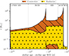 |
Fig. 2. Kippenhahn diagram of the evolutionary stages of a MZAMS = 1 M⊙ star. All stellar evolutionary phases are indicated at the top. The dotted yellow region illustrates the radiative regions, and the brown hatched region illustrates the convective regions. Stellar evolutionary phases (pre-MS to WD) are indicated. |
3.1.2. Angular momentum luminosities
The angular momentum luminosities carried by stochastically excited and tidally excited gravity waves are shown in Fig. 3 for a Jupiter-mass companion with an orbital period of 1 year (used for illustrative purposes, a companion further than the maximal radius of the host star). The stochastic excitation dominates the tidal excitation during the entire evolution of the star, but this is strongly dependent on the orbital period, which is investigated further in later sections.
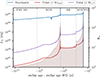 |
Fig. 3. Angular momentum luminosities carried by stochastically (blue) and tidally (red and purple) excited gravity waves (left axis) and stellar radius (brown; right axis) as a function of stellar age for a MZAMS = 1 M⊙ star with a 1 MJup (red) and a 1 M⊙ (purple) companion orbiting at 1 AU. Stellar evolutionary phases (pre-MS to WD) are indicated. |
Overall, the angular momentum luminosity carried by stochastically excited gravity waves is rather constant (compared to the angular momentum luminosity carried by tidally excited gravity waves), increasing from 1037 erg during the MS to 1040 erg when the star enters later evolutionary phases. During the entire evolution the luminosity is dominated by the waves excited from the convective envelope to the radiative core, except during the helium flash where the intense luminous flash increases the convective velocity in the convective core by several orders of magnitude. This results in a short spike in the convective velocity at the convective–radiative interface of the core. This spike results in a short burst in the angular momentum luminosity, although this burst does not last long enough to contribute to the overall transport. To demonstrate the influence of the other physical parameters, the evolution of the relevant parameters for the angular momentum luminosity (see Eq. 10) is presented in Fig. 4. Here, the convective velocity (dashed red) and the density at the interface (solid orange) mostly dominate changes in the angular momentum luminosity. They are anti-correlated, which can be understood by looking at the definition of the convective velocity in the standard MLT as vc3 = L★/(ρCZR★2). The remaining dominant factor in the convective velocity is the stellar luminosity, which increases during the later evolutionary phases. Therefore, the convective velocity will also gradually increase throughout the later evolutionary phases compared to the local density at the interface, and thus the angular momentum luminosity carried by stochastically excited gravity waves will increase as well.
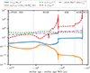 |
Fig. 4. Different parameters influencing the angular momentum luminosity carried by stochastically excited gravity waves (Eq. 10) as a function of stellar age for a MZAMS = 1 M⊙ star. Shown are the changes in: the radius of the radiative–convective boundary (solid blue), density (solid orange), convective timescale (dashed green), convective velocity (dashed red), Brunt-Väisälä frequency (dash-dotted purple), and Brunt-Väisälä frequency squared (dash-dotted brown) at the radiative-convective boundary. Stellar evolutionary phases (pre-MS to WD) are indicated. |
The angular momentum luminosity carried by tidally excited gravity waves is much lower than the stochastic excitation (in the case of Porb = 1 year) but increases more drastically during the later evolutionary phases. The evolution of the relevant parameters influencing this angular momentum luminosity (see Eq. 14) is shown in Fig. 5. Here it can be seen that the tidal forcing is the dominant factor, and it increases by multiple orders of magnitude during the evolved phases. The strongest component influencing the tidal forcing evolution is the evolution of the stellar radius, because the tidal forcing (ℱ) is dependent on R★5 (see Esseldeurs et al. 2024 and Appendix B). This is counteracted a bit by the density at the interface, which decreases during the evolved phases, but not enough to counteract the increase in the tidal forcing.
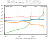 |
Fig. 5. Different parameters influencing the angular momentum luminosity carried by tidally excited gravity waves (Eq. 14) as a function of stellar age for a MZAMS = 1 M⊙ star with a 1 MJup companion orbiting at 1 AU. Shown are the change in radius of the radiative–convective boundary (solid blue), the change in density at this radius (solid orange), the change in tidal forcing (dashed green), and the change in the Brunt-Väisälä frequency squared (dash-dotted red). Stellar evolutionary phases (pre-MS to WD) are indicated. |
3.1.3. The case of star–planet systems
For an orbital period of 1 year (used for illustrative purposes, a companion further than the maximal radius of the host star), a Jupiter-mass planet will not have a significant impact on the angular momentum luminosities inside the star. This, however, strongly depends on the orbital period of the object. This can be seen in Figs. 6 and 7, where the angular momentum luminosity carried by stochastically (Fig. 6) and tidally (Fig. 7) excited gravity waves is shown as a function of stellar age and orbital period. Here the Roche limit (in purple) as well as the critical period (in orange) are plotted. The Roche limit represents the radius (or orbital period) at which the tidal forces on the planet are sufficiently strong to disrupt the planet (for the calculation, we refer to Benbakoura et al. 2019). The angular momentum carried by tidally excited gravity waves depends on the tidal frequency (and thus the orbital frequency) to the power of 8/3 (see Eq. 14). Therefore, when the orbital period decreases, the orbital frequency and thus the tidal frequency increase, increasing the tidal angular momentum luminosity. The ratio of the angular momentum luminosity carried by tidally excited gravity waves to the angular momentum luminosity carried by stochastically excited gravity waves is shown in Fig. 8. Here it can be seen that for a Jupiter-mass companion the stochastic excitations completely dominate over tidal excitations in most of the parameter space. However, for orbital periods shorter than about a day at the beginning of the RGB phase, the tidal excitation starts to have an influence. Although this is only a small part of the parameter space we explored, planets have been observed close to this regime (e.g. Jones et al. 2014; Saunders et al. 2024).
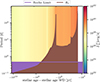 |
Fig. 6. Angular momentum luminosity carried by stochastically excited gravity waves (Eq. 10) as a function of stellar age for a MZAMS = 1 M⊙ star and the orbital period of a 1 MJup companion. R★ (in brown) represents the orbital period on which a companion orbits at the surface of the star, and the Roche limit is given in purple. Changes in the stellar evolutionary phase are indicated with ticks on the upper axis. |
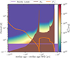 |
Fig. 7. Angular momentum luminosity carried by tidally excited gravity waves (Eq. 14) as a function of stellar age for a MZAMS = 1 M⊙ star and the orbital period of a 1 MJup companion. The critical period, Pc, above which companions excite progressive IGWs, is shown in orange. R★ (in brown) represents the orbital period on which a companion orbits at the surface of the star, and the Roche limit is given in purple. Changes in the stellar evolutionary phase are indicated with ticks on the upper axis. |
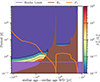 |
Fig. 8. Ratio of the angular momentum luminosity carried by tidally excited gravity waves (Eq. 14) to the angular momentum luminosity carried by stochastically excited gravity waves (Eq. 10) as a function of stellar age for a MZAMS = 1 M⊙ star with a Jupiter-mass companion. Contour lines are shown for ratios of 0.01, 0.1, 1, 10, and 100. The middle contour line with ratio 1 indicates the critical orbital period, Porb, crit, for this companion mass. The critical period, Pc, above which companions excite progressive IGWs, is shown in orange. R★ (in brown) represents the orbital period on which a companion orbits at the surface of the star, and the Roche limit is given in purple. Changes in the stellar evolutionary phase are indicated with ticks on the upper axis. |
3.1.4. The case of binary stars
When the mass of the companion increases, so will the angular momentum luminosity of the tidal excitation. This can be seen in Fig. 9, where ratio of the angular momentum luminosity carried by tidally excited gravity waves to the angular momentum luminosity carried by stochastically excited gravity waves is shown as a function of orbital period for a solar-mass companion. Here the stellar Roche limit (distance at which the primary overfills its Roche lobe) is plotted rather than the Roche limit (distance at which the companion overfills its Roche lobe). In the figure it can be seen that the tidal excitation starts to contribute earlier, during the MS with orbital periods of a few days, and during the RGB with a period of just under 10 days. During the HB phase, the tidal excitations start to contribute for orbital periods of just under 30 days (a contribution larger than 1%), but to have an equal ratio the companion would have to be inside the stellar Roche limit.
3.1.5. Critical mass
This information about planetary and stellar companions can be combined using the critical mass. The critical mass as a function of orbital period and stellar age is shown in Fig. 10. Here both the stellar and planetary Roche limits are plotted. Contour lines are also shown for one Earth mass, one Jupiter mass, and one solar mass. The contour for the Earth mass does not show up in the diagram, indicating that an earth mass will never be able to excite gravity waves with an angular momentum luminosity larger than the already stochastically excited gravity waves. The Jupiter-mass contour rises above its Roche limit at the beginning of the RGB phase (consistent with Sect. 3.1.3), and the stellar mass contour ranges from 2 to 5 days in the MS and the beginning of the RGB, but during the HB it is not able to reach above its Roche limit (consistent with Sect. 3.1.4).
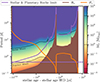 |
Fig. 10. Critical mass as a function of the orbital period and stellar age for a MZAMS = 1 M⊙ star. Contour lines are shown for MEarth, MJupiter, and M⊙ companions. These contour lines also indicate their critical orbital period. The critical period, Pc, is shown in orange. The R★ is shown in brown and the stellar and planetary Roche limit in purple. Contour lines are shown for 1 MEarth, 1 MJupiter, and 1 M⊙. Changes in the stellar evolutionary phase are indicated with ticks on the upper axis. |
3.2. Early-type binary stars
3.2.1. Internal structure
For stars with higher initial masses, the internal structure is different. The Kippenhahn diagram for a MZAMS = 2 M⊙ star is shown in Fig. 11 (top left). The star has a convective core and a radiative envelope during the MS phase. When the hydrogen in the core is depleted, the star turns into an RGB star, similar to the 1 M⊙ star (see Sect. 3.1.1) following the same later evolution. The star has a helium flash at the end of the RGB turning it into a HB star, and then into an AGB star. The star loses mass during the RGB and AGB phases, and eventually becomes a WD.
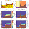 |
Fig. 11. Internal structure and angular momentum luminosities for a MZAMS = 2 M⊙ star. Top left: Kippenhahn diagram. The brown hatched regions represent convective layers, and the dotted yellow region represents radiative layers. Stellar evolutionary phases (pre-MS to WD) are indicated. Top right and centre left: Angular momentum luminosities carried by stochastically and tidally excited gravity waves as a function of orbital period and stellar age. Center right and bottom left: Ratio of the angular momentum luminosity carried by tidally excited waves to the angular momentum luminosity carried by stochastically excited waves as a function of orbital period and stellar age for a 1 MJup (centre right) and a 1 M⊙ (bottom left) companion. Bottom right: Critical mass as a function of orbital period and stellar age. The Roche limit is shown in purple, the critical period (4π/ωc; see Eq. 2) in orange, and the period at which a planet orbits at the stellar radius in brown. Changes in the stellar evolutionary phase are indicated with ticks on the upper axis. |
3.2.2. Angular momentum luminosities
The angular momentum luminosities carried by stochastically and tidally excited gravity waves are shown in Fig. 11 (top right and middle left panel, respectively). Similar to the 1 M⊙ star, the stochastic excitation remains (compared to the angular momentum luminosity carried by tidally excited gravity waves), with a slight increase from 1039 erg during the MS to 1040 erg when the star enters later evolutionary phases. Here, however, there is a short time during the transition from MS to RGB when the angular momentum luminosity drops by 4 orders of magnitude. During the MS the angular momentum luminosity is dominated by the contribution from the convective core, as the star has a negligible convective envelope. At the end of the MS this convective core disappears, while the convective envelope only appears during the RGB phase itself. Therefore, there is a transition period where there only is a negligible convective envelope, and no convective core.
The angular momentum luminosity carried by tidally excited gravity waves during the MS is negligible compared to the angular momentum luminosity carried by stochastic excitation. During the RGB when the convective envelope appears, the angular momentum luminosity carried by tidally excited gravity waves increases, but remains relatively low during its entire evolution.
3.2.3. The case of star–planet systems
For a Jupiter-mass companion, the angular momentum carried by tidally excited gravity waves is negligible compared to the angular momentum carried by stochastically excited waves during the entire evolution. This can be seen in Fig. 11 (middle left panel), where the ratio of the angular momentum luminosity carried by tidally excited gravity waves to the angular momentum luminosity carried by stochastically excited gravity waves is shown as a function of stellar age.
3.2.4. The case of binary stars
For a solar-mass companion, the angular momentum carried by tidally excited gravity waves is negligible compared to the angular momentum carried by stochastically excited waves during most of the evolution. This can be seen in Fig. 11 (bottom left panel) where the ratio of the angular momentum luminosity carried by tidally excited gravity waves to the angular momentum luminosity carried by stochastically excited gravity waves is shown as a function of orbital period for a solar-mass companion. Here, however, at the beginning of the RGB, as well as close to the stellar Roche limit during the HB phase, the tidal excitations starts to compete. This region of the parameter space, however, is so close to the host star that these systems are not long-lived, and therefore not relevant for the evolution of the star.
A few observed early-type stars in close binaries have measured internal rotation rates from asteroseismology (e.g. Beck et al. 2018; Van Reeth et al. 2022; Michielsen et al. 2023). In particular KIC 4930889, studied by Michielsen et al. (2023), is a 4 M⊙ star with a 3 M⊙ companion in an 18-day orbit. In their study they investigated the necessity of additional convective boundary mixing and angular momentum transport on top of the transport by stochastically excited gravity waves; they found a preference for either an exponentially decaying mixing profile in the near-core region or the absence of additional near-core mixing. This is consistent with our findings that the tidal excitation of gravity waves is negligible compared to the stochastic excitation for this system.
4. Discussion
4.1. Transport of angular momentum
Given the results from Sect. 3, it is clear that the stochastic excitation of gravity waves dominates over their tidal excitation for most of the parameter space. Only for very close-in stellar companions around late-type stars does the tidal excitation start to compete with the stochastic excitation. For early-type stars, the tidal excitation of gravity waves is negligible during the entire evolution, when compared to the stochastic excitation.
This result has key implications. First of all, the presence of a companion will not significantly increase the angular momentum transport by gravity waves in the host star on evolutionary timescales, except for very close-in stellar companions. Once excited by a source term, an IGW will transport and redistribute angular momentum in the same way independently of its excitation mechanism (we refer the reader to Talon & Charbonnel 2005 for stochastically excited waves and to Goldreich & Nicholson 1989; Talon & Kumar 1998 for tidally excited waves). Depending on the gradient of angular velocity between the place where they are excited and the propagation region we consider, and their prograde or retrograde behaviour, they will deposit or extract angular momentum in the considered stellar radiation zone (for instance, a retrograde wave propagating in the radiative core of a solar-type star with a core rotating faster than the envelope will extract angular momentum). In this framework, the torques applied on the surrounding convective envelope by stellar winds, the equilibrium tide and tidal inertial waves in the case of late-type stars are essential since they are the source of the rotation gradient that leads to a net deposit or extraction of angular momentum from the radiative core. As shown by Goldreich & Nicholson (1989) and Ahuir et al. (2021a), the net global torque applied on the radiative region is then directly related to the wave angular momentum luminosity at the place of its excitation. Therefore, the redistribution of angular momentum by internal waves is a function of their angular momentum luminosity at the radiative–convective interface where they are excited (which is dominated by the stochastic excitation in a broad parameter space) and of the gradient between the rotation of the place we study in a stellar radiation zone and the rotation of the surrounding stellar convective envelope or surface, which results from the action of stellar winds and the equilibrium tide and tidal inertial waves in the case of a convective envelope (Ahuir et al. 2021b). If the torque applied by stellar winds dominates tidal torques while the stochastic excitation dominate the tidal one, the rotational evolution of a star will be weakly affected by the presence of the companion. This means that the presence of a companion will not help explain the observed rotation rates of stellar cores in evolved stars, and other mechanisms are still needed to explain these observations. Second, as planetary companions do not significantly affect the angular momentum transport in the cores of their host stars, it is still possible to approximate the core rotational evolution of the host star without taking into account the presence of the planet2. This is especially useful when comparing asteroseismological observations to stellar evolution models, as the impact of a planet can be neglected for the internal wave-driven transport of angular momentum. Finally, as the tidal excitation of gravity waves is negligible in comparison with their stochastic excitation for most of the parameter space, it is not necessary to include this mechanism systematically in stellar evolution codes that already include the stochastic excitation of gravity waves (Charbonnel et al. 2013; Mathis 2013; Fuller et al. 2014). This simplifies the implementation of angular momentum transport by gravity waves in these codes. However, the dissipation of tides will still be crucial because it is the sole vector that conveys global exchanges of angular momentum between the spin of the star and the orbit of its companion.
4.2. Impact of the Coriolis acceleration
The rotation of the star impacts the excitation, propagation, and damping of both stochastically excited and tidally excited waves (e.g. Ogilvie & Lin 2004, 2007; Mathis 2009; Mathis et al. 2014). First, in convective regions, for sub-inertial frequencies (frequencies below the inertial frequency 2Ω), evanescent gravity waves found in the non-rotating case are replaced by propagative inertial waves that will be excited both by tides (e.g. Ogilvie & Lin 2004, 2007) and by turbulent convective Reynolds stresses (e.g. Bekki et al. 2022; Philidet & Gizon 2023; Blume et al. 2024; Fuentes et al. 2026). The properties of inertial modes propagating in a spherical shell such as stellar convective envelopes require multi-dimensional numerical simulations since the problem is bi-dimensional and non-separable (Rieutord & Valdettaro 1997; Bekki et al. 2022). Such heavy multi-dimensional simulations are also required to compute their excitation by tides and by turbulent convection (Ogilvie & Lin 2004, 2007; Bekki et al. 2022; Blume et al. 2024; Fuentes et al. 2026). Analytical treatments of the tidal excitation and stochastic excitation are possible but at the price of strong assumptions such as an average over all possible tidal frequencies (and periods; Ogilvie 2013) for the tidal excitation or of complex formalisms for the stochastic excitation (Augustson et al. 2020; Neiner et al. 2020; Philidet & Gizon 2023). In the case of super-inertial frequencies, the complexity also increases with gravito-inertial waves, which are evanescent as gravity waves in the non-rotating case but with an evanescence that now depends on rotation (e.g. Mathis et al. 2014). As a consequence, it is not yet possible to compare in a tractable and robust way the amplitude of tidally excited and stochastically excited waves propagating in stellar convective regions for the broad space of stellar and orbital parameters explored here. The same is true in stellar radiation zones where gravity waves become gravito-inertial waves with more complex propagation and damping as a function of the stratification and rotation (e.g. Lee & Saio 1997; Mathis 2009; Mirouh et al. 2016; Mathis 2026). Their tidal excitation becomes also more complex because of their couplings with tidal inertial waves at radiation/convection boundaries (Ogilvie & Lin 2004; Dhouib et al. 2024) that require the same multi-dimensional numerical treatment that in stellar convective envelopes. Concerning the treatment of the stochastic excitation of gravito-inertial waves by turbulent motions in the adjacent convective regions, progresses have been achieved (Mathis et al. 2014; Augustson et al. 2020; Neiner et al. 2020). However, the variation in its strength as a function of rotation is complex. For instance, it decreases with increasing rotation for the radiative–convective interface excitation while it can increase for their excitation by Reynolds stresses in the bulk of convective regions (Augustson et al. 2020). These results have been obtained within a monochromatic approach, where the wave period is close to the characteristic convective turn-over time, and it must be extended to understand the possible impact of the turbulent spectrum. Taking into account the impact of rotation on the excitation, propagation, and damping of both stochastically excited and tidally excited waves is therefore a complex task that requires multi-dimensional numerical simulations and/or complex analytical treatments. This is beyond the scope of this paper but will be investigated in future work.
5. Conclusion
In this work we computed the angular momentum luminosities carried by stochastically and tidally excited gravity waves in stars with different initial masses. The angular momentum luminosity carried by stochastically excited gravity waves is much higher than that carried by tidally excited waves, and it strongly depends on the orbital period of the companion. For a 1 M⊙ star with a Jupiter-mass companion, the tidal excitation of gravity waves only starts to compete with the stochastic excitation during the beginning of the RGB phase for orbital periods shorter than a day. For a solar-mass companion, the tidal excitation of gravity waves only starts to compete with the stochastic excitation during the MS and RGB phases for orbital periods shorter than a few days. We also computed the critical mass of the companion, which shows the same trend. For a 2 M⊙ star, the tidal excitation of gravity waves is negligible when compared to the stochastic one during the entire evolution.
Overall, our results suggest that while tidally excited IGWs are an interesting theoretical phenomenon and are important for tidal interactions and the related orbital evolution, they do not play a major role in shaping the internal angular momentum evolution of low- and intermediate-mass stars with companions. Instead, stochastic excitation by convection remains the dominant IGW-driving mechanism. This will simplify forthcoming stellar modelling efforts, as the presence of companions can be neglected when studying IGW-driven angular momentum transport in stars.
Note, however, that it still remains necessary to take into account tidal torques applied to the convective envelope due to the equilibrium tide (Zahn 1966, 1989; Remus et al. 2012) and to tidal inertial waves (Ogilvie & Lin 2004; Mathis 2015; Barker 2020), which can compete with the torque applied by stellar winds (Barker & Ogilvie 2009; Madappatt et al. 2016; Ahuir et al. 2021b). In addition, this picture should be refined by considering the impact of both rotation and magnetic fields on the excitation, propagation, and damping of stochastically and tidally excited magneto-gravito-inertial waves (e.g. Ogilvie & Lin 2004, 2007; Mathis 2009; Mathis & de Brye 2012; Lin & Ogilvie 2018; Augustson et al. 2020; Bessila & Mathis 2024).
Data availability
The data underlying this article will be shared on reasonable request to the corresponding author. The stellar evolutionary models used in this work can be found on Zenodo: https://doi.org/10.5281/zenodo.11519523, and additional figures containing the energy or angular momentum luminosities for all the stellar masses can be found on Zenodo: https://zenodo.org/records/19257979
Acknowledgments
The authors would like to thank the anonymous referee for their constructive comments which helped to improve the quality of the paper. M. Esseldeurs, S. Mathis and L. Decin acknowledge support from the FWO grant G0B3823N. M. Esseldeurs and L. Decin acknowledge support from the FWO grant G099720N, the KU Leuven C1 excellence grant MAESTRO C16/17/007, the KU Leuven IDN grant ESCHER IDN/19/028 and the KU Leuven methusalem SOUL grant METH/24/012. S. Mathis acknowledges support from the PLATO CNES grant at CEA/DAp, from the Programme National de Planétologie (PNP-CNRS/INSU) and from the European Research Council through HORIZON ERC SyG Grant 4D-STAR 101071505. L. Decin acknowledges support from the FWO sabbatical grant K803625N. While partially funded by the European Union, views and opinions expressed are however those of the author only and do not necessarily reflect those of the European Union or the European Research Council. Neither the European Union nor the granting authority can be held responsible for them.
References
- Aerts, C., Christensen-Dalsgaard, J., & Kurtz, D. W. 2010, Asteroseismology (Dordrecht: Springer) [Google Scholar]
- Aerts, C., Mathis, S., & Rogers, T. M. 2019, ARA&A, 57, 35 [Google Scholar]
- Aerts, C., Augustson, K., Mathis, S., et al. 2021, A&A, 656, A121 [NASA ADS] [CrossRef] [EDP Sciences] [Google Scholar]
- Aerts, C., Van Reeth, T., Mombarg, J. S. G., & Hey, D. 2025, A&A, 695, A214 [NASA ADS] [CrossRef] [EDP Sciences] [Google Scholar]
- Ahuir, J., Mathis, S., & Amard, L. 2021a, A&A, 651, A3 [NASA ADS] [CrossRef] [EDP Sciences] [Google Scholar]
- Ahuir, J., Strugarek, A., Brun, A. S., & Mathis, S. 2021b, A&A, 650, A126 [NASA ADS] [CrossRef] [EDP Sciences] [Google Scholar]
- Alvan, L., Brun, A. S., & Mathis, S. 2014, A&A, 565, A42 [NASA ADS] [CrossRef] [EDP Sciences] [Google Scholar]
- Alvan, L., Strugarek, A., Brun, A. S., Mathis, S., & Garcia, R. A. 2015, A&A, 581, A112 [NASA ADS] [CrossRef] [EDP Sciences] [Google Scholar]
- Anders, E. H., Lecoanet, D., Cantiello, M., et al. 2023, Nat. Astron., 7, 1228 [NASA ADS] [CrossRef] [Google Scholar]
- Asplund, M., Grevesse, N., Sauval, A. J., & Scott, P. 2009, ARA&A, 47, 481 [NASA ADS] [CrossRef] [Google Scholar]
- Augustson, K. C., Mathis, S., & Astoul, A. 2020, ApJ, 903, 90 [NASA ADS] [CrossRef] [Google Scholar]
- Baglin, A., Auvergne, M., Barge, P., et al. 2006, ESA Spec. Publ., 1306, 33 [Google Scholar]
- Barker, A. J. 2020, MNRAS, 498, 2270 [Google Scholar]
- Barker, A. J., & Ogilvie, G. I. 2009, MNRAS, 395, 2268 [NASA ADS] [CrossRef] [Google Scholar]
- Barrère, P., Reboul-Salze, A., Eggenberger, P., et al. 2026, A&A, submitted [arXiv:2601.02129] [Google Scholar]
- Beck, P. G., Montalban, J., Kallinger, T., et al. 2012, Nature, 481, 55 [Google Scholar]
- Beck, P. G., Kallinger, T., Pavlovski, K., et al. 2018, A&A, 612, A22 [NASA ADS] [CrossRef] [EDP Sciences] [Google Scholar]
- Beck, P. G., Mathur, S., Hambleton, K., et al. 2022, A&A, 667, A31 [NASA ADS] [CrossRef] [EDP Sciences] [Google Scholar]
- Bekki, Y., Cameron, R. H., & Gizon, L. 2022, A&A, 662, A16 [NASA ADS] [CrossRef] [EDP Sciences] [Google Scholar]
- Belkacem, K., Mathis, S., Goupil, M. J., & Samadi, R. 2009, A&A, 508, 345 [NASA ADS] [CrossRef] [EDP Sciences] [Google Scholar]
- Benbakoura, M., Réville, V., Brun, A. S., Le Poncin-Lafitte, C., & Mathis, S. 2019, A&A, 621, A124 [NASA ADS] [CrossRef] [EDP Sciences] [Google Scholar]
- Bessila, L., & Mathis, S. 2024, A&A, 690, A270 [NASA ADS] [CrossRef] [EDP Sciences] [Google Scholar]
- Blöcker, T. 1995, A&A, 297, 727 [NASA ADS] [Google Scholar]
- Blume, C. C., Hindman, B. W., & Matilsky, L. I. 2024, ApJ, 966, 29 [Google Scholar]
- Bolmont, E., & Mathis, S. 2016, Celest. Mech. Dyn. Astron., 126, 275 [Google Scholar]
- Borucki, W. J., Koch, D., Basri, G., et al. 2010, Science, 327, 977 [Google Scholar]
- Bowman, D. M., & Bugnet, L. 2026, Encycl. Astrophys., 2, 133 [Google Scholar]
- Breton, S. N., Brun, A. S., & García, R. A. 2022, A&A, 667, A43 [NASA ADS] [CrossRef] [EDP Sciences] [Google Scholar]
- Brun, A. S., Strugarek, A., Varela, J., et al. 2017, ApJ, 836, 192 [Google Scholar]
- Cantiello, M., Mankovich, C., Bildsten, L., Christensen-Dalsgaard, J., & Paxton, B. 2014, ApJ, 788, 93 [Google Scholar]
- Ceillier, T., Eggenberger, P., García, R. A., & Mathis, S. 2013, A&A, 555, A54 [NASA ADS] [CrossRef] [EDP Sciences] [Google Scholar]
- Charbonnel, C., & Talon, S. 2005, Science, 309, 2189 [Google Scholar]
- Charbonnel, C., Decressin, T., Amard, L., Palacios, A., & Talon, S. 2013, A&A, 554, A40 [NASA ADS] [CrossRef] [EDP Sciences] [Google Scholar]
- Christensen-Dalsgaard, J. 2021, Liv. Rev. Sol. Phys., 18, 2 [NASA ADS] [CrossRef] [Google Scholar]
- Cinquegrana, G. C., & Joyce, M. 2022, Res. Notes Am. Astron. Soc., 6, 77 [Google Scholar]
- Couston, L.-A., Lecoanet, D., Favier, B., & Le Bars, M. 2018, J. Fluid Mech., 854, R3 [NASA ADS] [CrossRef] [Google Scholar]
- Daniel, F., & Lecoanet, D. 2026, J. Fluid Mech., 1028, A38 [Google Scholar]
- Deheuvels, S., García, R. A., Chaplin, W. J., et al. 2012, ApJ, 756, 19 [Google Scholar]
- Deheuvels, S., Doğan, G., Goupil, M. J., et al. 2014, A&A, 564, A27 [NASA ADS] [CrossRef] [EDP Sciences] [Google Scholar]
- Dhouib, H., Baruteau, C., Mathis, S., et al. 2024, A&A, 682, A85 [NASA ADS] [CrossRef] [EDP Sciences] [Google Scholar]
- Edelmann, P. V. F., Ratnasingam, R. P., Pedersen, M. G., et al. 2019, ApJ, 876, 4 [NASA ADS] [CrossRef] [Google Scholar]
- Eggenberger, P., Maeder, A., & Meynet, G. 2005, A&A, 440, L9 [NASA ADS] [CrossRef] [EDP Sciences] [Google Scholar]
- Eggenberger, P., Montalbán, J., & Miglio, A. 2012, A&A, 544, L4 [NASA ADS] [CrossRef] [EDP Sciences] [Google Scholar]
- Eggenberger, P., Buldgen, G., Salmon, S. J. A. J., et al. 2022a, Nat. Astron., 6, 788 [NASA ADS] [CrossRef] [Google Scholar]
- Eggenberger, P., Moyano, F. D., & den Hartogh, J. W. 2022b, A&A, 664, L16 [NASA ADS] [CrossRef] [EDP Sciences] [Google Scholar]
- Esseldeurs, M., Mathis, S., & Decin, L. 2024, A&A, 690, A266 [NASA ADS] [CrossRef] [EDP Sciences] [Google Scholar]
- Esseldeurs, M., Decin, L., De Ridder, J., et al. 2026, Nat. Astron., 10, 124 [Google Scholar]
- Fuentes, J. R., Barik, A., & Fuller, J. 2026, ApJ, 998, 131 [Google Scholar]
- Fuller, J., Lecoanet, D., Cantiello, M., & Brown, B. 2014, ApJ, 796, 17 [Google Scholar]
- Fuller, J., Piro, A. L., & Jermyn, A. S. 2019, MNRAS, 485, 3661 [NASA ADS] [Google Scholar]
- Gallet, F., Bolmont, E., Mathis, S., Charbonnel, C., & Amard, L. 2017, A&A, 604, A112 [NASA ADS] [CrossRef] [EDP Sciences] [Google Scholar]
- Garcia Lopez, R. J., & Spruit, H. C. 1991, ApJ, 377, 268 [NASA ADS] [CrossRef] [Google Scholar]
- García, R. A., & Ballot, J. 2019, Liv. Rev. Sol. Phys., 16, 4 [Google Scholar]
- Gehan, C., Mosser, B., Michel, E., Samadi, R., & Kallinger, T. 2018, A&A, 616, A24 [NASA ADS] [CrossRef] [EDP Sciences] [Google Scholar]
- Goldreich, P., & Kumar, P. 1990, ApJ, 363, 694 [NASA ADS] [CrossRef] [Google Scholar]
- Goldreich, P., & Nicholson, P. D. 1989, ApJ, 342, 1079 [Google Scholar]
- Goodman, J., & Dickson, E. S. 1998, ApJ, 507, 938 [Google Scholar]
- Henyey, L., Vardya, M. S., & Bodenheimer, P. 1965, ApJ, 142, 841 [Google Scholar]
- Herwig, F., Woodward, P. R., Mao, H., et al. 2023, MNRAS, 525, 1601 [NASA ADS] [CrossRef] [Google Scholar]
- Hinkel, N. R., Youngblood, A., & Soares-Furtado, M. 2024, Rev. Mineral. Geochem., 90, 1 [Google Scholar]
- Jermyn, A. S., Bauer, E. B., Schwab, J., et al. 2023, ApJS, 265, 15 [NASA ADS] [CrossRef] [Google Scholar]
- Jones, M. I., Jenkins, J. S., Bluhm, P., Rojo, P., & Melo, C. H. F. 2014, A&A, 566, A113 [NASA ADS] [CrossRef] [EDP Sciences] [Google Scholar]
- Le Saux, A., Guillet, T., Baraffe, I., et al. 2022, A&A, 660, A51 [NASA ADS] [CrossRef] [EDP Sciences] [Google Scholar]
- Lecoanet, D., & Quataert, E. 2013, MNRAS, 430, 2363 [Google Scholar]
- Lee, U., & Saio, H. 1997, ApJ, 491, 839 [Google Scholar]
- Li, G., Van Reeth, T., Bedding, T. R., et al. 2020, MNRAS, 491, 3586 [Google Scholar]
- Lin, Y., & Ogilvie, G. I. 2018, MNRAS, 474, 1644 [Google Scholar]
- Madappatt, N., De Marco, O., & Villaver, E. 2016, MNRAS, 463, 1040 [NASA ADS] [CrossRef] [Google Scholar]
- Marigo, P., & Aringer, B. 2009, A&A, 508, 1539 [CrossRef] [EDP Sciences] [Google Scholar]
- Marques, J. P., Goupil, M. J., Lebreton, Y., et al. 2013, A&A, 549, A74 [NASA ADS] [CrossRef] [EDP Sciences] [Google Scholar]
- Mathis, S. 2009, A&A, 506, 811 [CrossRef] [EDP Sciences] [Google Scholar]
- Mathis, S. 2013, Lect. Notes Phys., 865, 23 [Google Scholar]
- Mathis, S. 2015, A&A, 580, L3 [EDP Sciences] [Google Scholar]
- Mathis, S. 2018, in Handbook of Exoplanets, eds. H. J. Deeg, & J. A. Belmonte (Springer International Publishing AG), 24 [Google Scholar]
- Mathis, S. 2026, A&A, 706, A71 [NASA ADS] [CrossRef] [EDP Sciences] [Google Scholar]
- Mathis, S., & de Brye, N. 2012, A&A, 540, A37 [NASA ADS] [CrossRef] [EDP Sciences] [Google Scholar]
- Mathis, S., Neiner, C., & Tran Minh, N. 2014, A&A, 565, A47 [NASA ADS] [CrossRef] [EDP Sciences] [Google Scholar]
- McDonald, I., & Zijlstra, A. A. 2015, MNRAS, 448, 502 [Google Scholar]
- Michielsen, M., Van Reeth, T., Tkachenko, A., & Aerts, C. 2023, A&A, 679, A6 [NASA ADS] [CrossRef] [EDP Sciences] [Google Scholar]
- Mirouh, G. M., Baruteau, C., Rieutord, M., & Ballot, J. 2016, J. Fluid Mech., 800, 213 [NASA ADS] [CrossRef] [Google Scholar]
- Mosser, B., Goupil, M. J., Belkacem, K., et al. 2012, A&A, 548, A10 [NASA ADS] [CrossRef] [EDP Sciences] [Google Scholar]
- Mulders, G. D., Pascucci, I., Apai, D., & Ciesla, F. J. 2018, AJ, 156, 24 [Google Scholar]
- Neiner, C., Lee, U., Mathis, S., et al. 2020, A&A, 644, A9 [EDP Sciences] [Google Scholar]
- Ogilvie, G. I. 2013, MNRAS, 429, 613 [Google Scholar]
- Ogilvie, G. I. 2014, ARA&A, 52, 171 [Google Scholar]
- Ogilvie, G. I., & Lin, D. N. C. 2004, ApJ, 610, 477 [Google Scholar]
- Ogilvie, G. I., & Lin, D. N. C. 2007, ApJ, 661, 1180 [Google Scholar]
- Ouazzani, R. M., Marques, J. P., Goupil, M. J., et al. 2019, A&A, 626, A121 [NASA ADS] [CrossRef] [EDP Sciences] [Google Scholar]
- Paxton, B., Bildsten, L., Dotter, A., et al. 2011, ApJS, 192, 3 [Google Scholar]
- Paxton, B., Cantiello, M., Arras, P., et al. 2013, ApJS, 208, 4 [Google Scholar]
- Paxton, B., Marchant, P., Schwab, J., et al. 2015, ApJS, 220, 15 [Google Scholar]
- Paxton, B., Schwab, J., Bauer, E. B., et al. 2018, ApJS, 234, 34 [NASA ADS] [CrossRef] [Google Scholar]
- Paxton, B., Smolec, R., Schwab, J., et al. 2019, ApJS, 243, 10 [Google Scholar]
- Petitdemange, L., Marcotte, F., & Gissinger, C. 2023, Science, 379, 300 [NASA ADS] [CrossRef] [Google Scholar]
- Philidet, J., & Gizon, L. 2023, A&A, 673, A124 [NASA ADS] [CrossRef] [EDP Sciences] [Google Scholar]
- Pinçon, C., Belkacem, K., & Goupil, M. J. 2016, A&A, 588, A122 [NASA ADS] [CrossRef] [EDP Sciences] [Google Scholar]
- Pinçon, C., Belkacem, K., Goupil, M. J., & Marques, J. P. 2017, A&A, 605, A31 [NASA ADS] [CrossRef] [EDP Sciences] [Google Scholar]
- Press, W. H. 1981, ApJ, 245, 286 [Google Scholar]
- Reimers, D. 1975, Problems in Stellar Atmospheres and Envelopes (Springer-Verlag), 229 [Google Scholar]
- Remus, F., Mathis, S., & Zahn, J. P. 2012, A&A, 544, A132 [NASA ADS] [CrossRef] [EDP Sciences] [Google Scholar]
- Ricker, G. R., Winn, J. N., Vanderspek, R., et al. 2015, J. Astron. Telesc. Instrum. Syst., 1, 014003 [Google Scholar]
- Rieutord, M., & Valdettaro, L. 1997, J. Fluid Mech., 341, 77 [Google Scholar]
- Rogers, T. M. 2015, ApJ, 815, L30 [Google Scholar]
- Rogers, T. M., Lin, D. N. C., McElwaine, J. N., & Lau, H. H. B. 2013, ApJ, 772, 21 [NASA ADS] [CrossRef] [Google Scholar]
- Sana, H., de Mink, S. E., de Koter, A., et al. 2012, Science, 337, 444 [Google Scholar]
- Saunders, N., Grunblatt, S. K., Chontos, A., et al. 2024, AJ, 168, 81 [Google Scholar]
- Schatzman, E. 1993, A&A, 279, 431 [NASA ADS] [Google Scholar]
- Song, H. F., Meynet, G., Maeder, A., Ekström, S., & Eggenberger, P. 2016, A&A, 585, A120 [NASA ADS] [CrossRef] [EDP Sciences] [Google Scholar]
- Spruit, H. C. 2002, A&A, 381, 923 [CrossRef] [EDP Sciences] [Google Scholar]
- Talon, S., & Charbonnel, C. 2005, A&A, 440, 981 [NASA ADS] [CrossRef] [EDP Sciences] [Google Scholar]
- Talon, S., & Kumar, P. 1998, ApJ, 503, 387 [Google Scholar]
- Tayler, R. J. 1973, MNRAS, 161, 365 [CrossRef] [Google Scholar]
- Van Reeth, T., Tkachenko, A., & Aerts, C. 2016, A&A, 593, A120 [NASA ADS] [CrossRef] [EDP Sciences] [Google Scholar]
- Van Reeth, T., Southworth, J., Van Beeck, J., & Bowman, D. M. 2022, A&A, 659, A177 [NASA ADS] [CrossRef] [EDP Sciences] [Google Scholar]
- Zahn, J. P. 1966, Ann. Astrophys., 29, 313 [NASA ADS] [Google Scholar]
- Zahn, J. P. 1975, A&A, 41, 329 [NASA ADS] [Google Scholar]
- Zahn, J. P. 1977, A&A, 57, 383 [Google Scholar]
- Zahn, J. P. 1989, A&A, 220, 112 [Google Scholar]
- Zahn, J.-P. 1991, A&A, 252, 179 [NASA ADS] [Google Scholar]
- Zahn, J. P. 1992, A&A, 265, 115 [NASA ADS] [Google Scholar]
- Zahn, J. P. 1994, A&A, 288, 829 [Google Scholar]
- Zahn, J. P., Talon, S., & Matias, J. 1997, A&A, 322, 320 [NASA ADS] [Google Scholar]
A small description can be found in Appendix A.
The envelope rotational evolution can still be affected by a planetary companion; see e.g. Benbakoura et al. (2019), Ahuir et al. (2021b).
The inlist used to compute the stellar evolutionary models can be found both in Esseldeurs et al. 2024 and on Zenodo: https://doi.org/10.5281/zenodo.11519523
Appendix A: Stellar evolution models
In order to calculate the energy and angular momentum luminosities of gravity waves, we need to know the internal structure of a star throughout its lifetime. For this we used the stellar evolutionary code Modules for Experiments in Stellar Astrophysics (MESA; Paxton et al. 2011, 2013, 2015, 2018, 2019; Jermyn et al. 2023) using the same parameters as was done in Esseldeurs et al. (2024)3 for stars at solar metallicity (Z = 0.0134; Asplund et al. 2009) with initial masses between 1 and 4 M⊙.
Starting from the pre-MS, the stellar evolutionary models were computed up to the WD stage, where they are terminated when the luminosity reaches L = 10−1 L⊙. Convection in the simulations is modelled using the MLT following the prescription of Henyey et al. (1965) with αMLT = 1.931 (Cinquegrana & Joyce 2022) and opacity tables dedicated for low-temperature molecular opacities necessary in the evolved phases of evolution (ÆSOPUS; Marigo & Aringer 2009). The atmosphere is simulated using a grey temperature-opacity relation based on the Eddington relation (Paxton et al. 2011). The mixing processes in the simulations are simplified dramatically to reduce the complexity of the models, and reduce the computational cost. In the radiative zones of the star a constant mixing coefficient Dmin = 10 cm2 s−1 is assumed for numerical stability.
During the evolved phases, mass loss is taken into account. For the RGB phase, the Reimers prescription (Reimers 1975) is used with a scaling factor of ηReimers = 0.477 (McDonald & Zijlstra 2015). Further in the evolution during the AGB phase the Blöcker prescription (Blöcker 1995) is used with a scaling factor of ηBlcker = 0.1 for masses above 2 M⊙ and ηBlcker = 0.05 for masses below 2 M⊙ (Madappatt et al. 2016).
Appendix B: Unitless tidal forcing
The tidal forcing (Eq. 15) is not a unitless quantity, as there are units in the tidal potential φT, the local gravity g0, and the integration over the radius r. To understand the scaling of the tidal forcing, we can rewrite it to separate the unitless part from the part with units. The tidal forcing can be written as
 (B.1)
(B.1)
where  is the unitless part of the tidal forcing given by
![Mathematical equation: $$ \begin{aligned} \tilde{\mathcal{F} }_{\rm out}&= \int _0^{\alpha }\left[\left(\frac{x^6}{m_r}\right)^{\prime \prime }-\frac{l(l+1)}{x^2}\left(\frac{x^6}{m_r}\right)\right] \frac{X_{1, \mathrm{out}}}{X_{1, \mathrm{out}}(\alpha )} \mathrm{d} x,\end{aligned} $$](/articles/aa/full_html/2026/05/aa58219-25/aa58219-25-eq25.gif) (B.2)
(B.2)
![Mathematical equation: $$ \begin{aligned} \tilde{\mathcal{F} }_{\rm in}&= \int _{\alpha _c}^1\left[\left(\frac{x^6}{m_r}\right)^{\prime \prime }-\frac{l(l+1)}{x^2}\left(\frac{x^6}{m_r}\right)\right] \frac{X_{1, \mathrm{in}}}{X_{1, \mathrm{in}}(\alpha _c)} \mathrm{d} x, \end{aligned} $$](/articles/aa/full_html/2026/05/aa58219-25/aa58219-25-eq26.gif) (B.3)
(B.3)
where x = r/R★ (the power 6 originates from the 2 that is already present in the tidal forcing, the 2 from the tidal potential, and the 2 from the local gravity), α = rout/R★ the envelope radius aspect ratio, αc = rin/R★ the core radius aspect ratio, and mr = Mr/M1 with Mr the mass coordinate as a function of radius. The tidal forcing therefore scales with the mass ratio of the companion to the star, the inverse of the semi-major axis cubed, and the radius of the star to the fifth power.
The unitless tidal forcing  is a complicated integral, but for all the models computed in this work (1 to 4 M⊙), it is shown in Fig. B.1 as a function of α = rin/R★. For high values of α (i.e. when the convective envelope is very thin), the tidal forcing decreases as X does not have the room to grow. Going towards low values of α (i.e. when the convective envelope is very thick), the tidal forcing also decreases as X targets the inner part of the integral, where x is small. This results in a peak in the tidal forcing around α ≈ 0.4, where the convective envelope is neither too thin nor too thick. For an order of magnitude estimate, the dimensionless tidal forcing can be approximated as (a rough fit by eye)
 (B.4)
(B.4)
 (B.5)
(B.5)
This approximation, shown in Fig. B.1, captures the overall behaviour of the tidal forcing quite well.
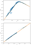 |
Fig. B.1. Unitless tidal forcing ( |

Appendix C: Froude number at the radiative–convective interface
The Froude number at the convective–radiative interface is an important parameter in the calculation of the angular momentum luminosity carried by stochastically excited gravity waves (see Eq. 10). It is either computed as ωc/Nint (in our approach following Press 1981) or approximated as vc/cs as proposed by Fuller et al. (2014), where cs is the sound speed at the interface, because of the uncertainties on the stratification in the convective penetration region (e.g. Zahn 1991; Pinçon et al. 2016). Their respective values are shown in Fig. C.1 for the 1 M⊙ stellar evolutionary model. The two definitions give differences up to 2 orders of magnitude. In the article, we can thus consider the Froude number computed as ωc/Nint as proposed here as a maximum value scenario while the Froude number computed as vc/cs is a minimal value scenario. When using the Froude number computed as vc/cs, the angular momentum luminosity carried by stochastically excited gravity waves will be lower by up to 2 orders of magnitude (as can be seen in Fig. C.2). Although this is a significant difference, the overall region of the parameter space where the tidal excitation starts to compete with the stochastic excitation will, however, not change significantly, as the dependance on the orbital period of the tidal excitation is so strong and our conclusions should be robust.
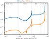 |
Fig. C.1. Froude number at the convective–radiative interface as a function of stellar age for a MZAMS = 1 M⊙ star. The Froude number computed as ωc/Nint is shown in blue, and the Froude number approximated as vc/cs is shown in orange. Stellar evolutionary phases (pre-MS to WD) are indicated. |
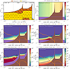 |
Fig. C.2. Same as Fig. 11 but using the Froude number approximated as vc/cs to compute the angular momentum luminosity carried by stochastically excited gravity waves. |
Appendix D: Energy luminosities
In Figs. D.1 and D.2 the internal structure and energy luminosities carried by both stochastically and tidally excited gravity waves for the 1 M⊙ and 2 M⊙ stellar evolutionary models, respectively, are shown.
All Figures
|
Fig. 1. Schematic view of the radiative and convective shells in the three-layer model used in this work. Radii are not to scale (see the Kippenhahn diagrams, e.g. Fig. 2). |
| In the text | |
|
Fig. 2. Kippenhahn diagram of the evolutionary stages of a MZAMS = 1 M⊙ star. All stellar evolutionary phases are indicated at the top. The dotted yellow region illustrates the radiative regions, and the brown hatched region illustrates the convective regions. Stellar evolutionary phases (pre-MS to WD) are indicated. |
| In the text | |
|
Fig. 3. Angular momentum luminosities carried by stochastically (blue) and tidally (red and purple) excited gravity waves (left axis) and stellar radius (brown; right axis) as a function of stellar age for a MZAMS = 1 M⊙ star with a 1 MJup (red) and a 1 M⊙ (purple) companion orbiting at 1 AU. Stellar evolutionary phases (pre-MS to WD) are indicated. |
| In the text | |
|
Fig. 4. Different parameters influencing the angular momentum luminosity carried by stochastically excited gravity waves (Eq. 10) as a function of stellar age for a MZAMS = 1 M⊙ star. Shown are the changes in: the radius of the radiative–convective boundary (solid blue), density (solid orange), convective timescale (dashed green), convective velocity (dashed red), Brunt-Väisälä frequency (dash-dotted purple), and Brunt-Väisälä frequency squared (dash-dotted brown) at the radiative-convective boundary. Stellar evolutionary phases (pre-MS to WD) are indicated. |
| In the text | |
|
Fig. 5. Different parameters influencing the angular momentum luminosity carried by tidally excited gravity waves (Eq. 14) as a function of stellar age for a MZAMS = 1 M⊙ star with a 1 MJup companion orbiting at 1 AU. Shown are the change in radius of the radiative–convective boundary (solid blue), the change in density at this radius (solid orange), the change in tidal forcing (dashed green), and the change in the Brunt-Väisälä frequency squared (dash-dotted red). Stellar evolutionary phases (pre-MS to WD) are indicated. |
| In the text | |
|
Fig. 6. Angular momentum luminosity carried by stochastically excited gravity waves (Eq. 10) as a function of stellar age for a MZAMS = 1 M⊙ star and the orbital period of a 1 MJup companion. R★ (in brown) represents the orbital period on which a companion orbits at the surface of the star, and the Roche limit is given in purple. Changes in the stellar evolutionary phase are indicated with ticks on the upper axis. |
| In the text | |
|
Fig. 7. Angular momentum luminosity carried by tidally excited gravity waves (Eq. 14) as a function of stellar age for a MZAMS = 1 M⊙ star and the orbital period of a 1 MJup companion. The critical period, Pc, above which companions excite progressive IGWs, is shown in orange. R★ (in brown) represents the orbital period on which a companion orbits at the surface of the star, and the Roche limit is given in purple. Changes in the stellar evolutionary phase are indicated with ticks on the upper axis. |
| In the text | |
|
Fig. 8. Ratio of the angular momentum luminosity carried by tidally excited gravity waves (Eq. 14) to the angular momentum luminosity carried by stochastically excited gravity waves (Eq. 10) as a function of stellar age for a MZAMS = 1 M⊙ star with a Jupiter-mass companion. Contour lines are shown for ratios of 0.01, 0.1, 1, 10, and 100. The middle contour line with ratio 1 indicates the critical orbital period, Porb, crit, for this companion mass. The critical period, Pc, above which companions excite progressive IGWs, is shown in orange. R★ (in brown) represents the orbital period on which a companion orbits at the surface of the star, and the Roche limit is given in purple. Changes in the stellar evolutionary phase are indicated with ticks on the upper axis. |
| In the text | |
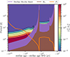 |
Fig. 9. Same as Fig. 8 but for a solar-mass companion. |
| In the text | |
|
Fig. 10. Critical mass as a function of the orbital period and stellar age for a MZAMS = 1 M⊙ star. Contour lines are shown for MEarth, MJupiter, and M⊙ companions. These contour lines also indicate their critical orbital period. The critical period, Pc, is shown in orange. The R★ is shown in brown and the stellar and planetary Roche limit in purple. Contour lines are shown for 1 MEarth, 1 MJupiter, and 1 M⊙. Changes in the stellar evolutionary phase are indicated with ticks on the upper axis. |
| In the text | |
|
Fig. 11. Internal structure and angular momentum luminosities for a MZAMS = 2 M⊙ star. Top left: Kippenhahn diagram. The brown hatched regions represent convective layers, and the dotted yellow region represents radiative layers. Stellar evolutionary phases (pre-MS to WD) are indicated. Top right and centre left: Angular momentum luminosities carried by stochastically and tidally excited gravity waves as a function of orbital period and stellar age. Center right and bottom left: Ratio of the angular momentum luminosity carried by tidally excited waves to the angular momentum luminosity carried by stochastically excited waves as a function of orbital period and stellar age for a 1 MJup (centre right) and a 1 M⊙ (bottom left) companion. Bottom right: Critical mass as a function of orbital period and stellar age. The Roche limit is shown in purple, the critical period (4π/ωc; see Eq. 2) in orange, and the period at which a planet orbits at the stellar radius in brown. Changes in the stellar evolutionary phase are indicated with ticks on the upper axis. |
| In the text | |
|
Fig. B.1. Unitless tidal forcing ( |
| In the text | |
|
Fig. C.1. Froude number at the convective–radiative interface as a function of stellar age for a MZAMS = 1 M⊙ star. The Froude number computed as ωc/Nint is shown in blue, and the Froude number approximated as vc/cs is shown in orange. Stellar evolutionary phases (pre-MS to WD) are indicated. |
| In the text | |
|
Fig. C.2. Same as Fig. 11 but using the Froude number approximated as vc/cs to compute the angular momentum luminosity carried by stochastically excited gravity waves. |
| In the text | |
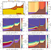 |
Fig. D.1. Same as Fig. 11 but for the energy luminosities and for a 1 M⊙ star. |
| In the text | |
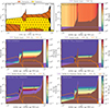 |
Fig. D.2. Same as Fig. 11 but for the energy luminosities. |
| In the text | |
Current usage metrics show cumulative count of Article Views (full-text article views including HTML views, PDF and ePub downloads, according to the available data) and Abstracts Views on Vision4Press platform.
Data correspond to usage on the plateform after 2015. The current usage metrics is available 48-96 hours after online publication and is updated daily on week days.
Initial download of the metrics may take a while.