| Issue |
A&A
Volume 709, May 2026
|
|
|---|---|---|
| Article Number | A267 | |
| Number of page(s) | 13 | |
| Section | Astronomical instrumentation | |
| DOI | https://doi.org/10.1051/0004-6361/202558504 | |
| Published online | 22 May 2026 | |
Focal plane wavefront control with model-based reinforcement learning
I. Proof of concept on simulated static and dynamic non-common path aberrations
1
European Southern Observatory (ESO),
Karl-Schwarzschild-Str. 2,
85748
Garching,
Germany
2
STAR Institute, Université de Liège,
Allée du Six Août 19C,
4000
Liège,
Belgium
★ Corresponding author: This email address is being protected from spambots. You need JavaScript enabled to view it.
Received:
10
December
2025
Accepted:
31
March
2026
Abstract
Context. The direct imaging of potentially habitable exoplanets is one prime science case for high-contrast imaging (HCI) instruments on ground-based, extremely large telescopes. Most such exoplanets orbit close to their host stars, where their observation is limited by fast-moving atmospheric speckles and quasi-static noncommon path aberrations (NCPA).
Aims. Conventional NCPA correction methods often use mechanical mirror probes, which compromise performance during operation. This work presents machine-learning-based NCPA control methods that automatically detect and correct both dynamic and static NCPA errors by leveraging past telemetry data and sequential phase diversity.
Methods. We extend previous work in reinforcement learning (RL) for adaptive optics (AO) to focal plane wavefront control. A new model-based RL algorithm, Policy Optimization for Noncommon Path Aberrations (PO4NCPA), interprets the focal plane image as input data and, through sequential phase diversity, determines phase corrections that optimize both non-coronagraphic and post-coronagraphic point spread functions (PSFs) without prior system knowledge. Furthermore, we demonstrate the effectiveness of this approach by numerically simulating static NCPA errors on a ground-based telescope and an infrared imager affected by water vapor-induced seeing (dynamic NCPAs).
Results. Simulations show that PO4NCPA robustly compensates static and dynamic NCPAs. In static cases, it achieves near-optimal focal plane light suppression with a coronagraph and near-optimal Strehl without one. With dynamic NCPA, it matches the performance of the modal least-squares reconstruction combined with a 1-step delay integrator in these metrics, though with a higher wavefront root mean square error (RMSE), especially for high-order modes. The method remains effective for the Extremely Large Telescope (ELT) pupil, the vector vortex coronagraph, under photon and background noise.
Conclusions. PO4NCPA is model-free and can be directly applied to standard imaging as well as to any type of coronagraphy; its submillisecond inference times and performance also make it suitable for real-time low-order correction of atmospheric turbulence beyond HCI requirements.
Key words: instrumentation: adaptive optics / instrumentation: high angular resolution / methods: data analysis / methods: numerical / techniques: imaging spectroscopy
F.R.S.-FNRS FRIA grantee.
F.R.S.-FNRS Research Director.
© The Authors 2026
 Open Access article, published by EDP Sciences, under the terms of the Creative Commons Attribution License (https://creativecommons.org/licenses/by/4.0), which permits unrestricted use, distribution, and reproduction in any medium, provided the original work is properly cited.
This article is published in open access under the Subscribe to Open model. This email address is being protected from spambots. You need JavaScript enabled to view it. to support open access publication.
1 Introduction
Studying extrasolar planets (exoplanets) and their systems is one of the fastest-growing areas in modern astrophysics. To date, more than 6000 confirmed exoplanets have been discovered, primarily using indirect methods such as radial velocity and photometric transit observations1. High-contrast imaging (HCI) aims to separate exoplanet light from stellar light optically, thereby allowing direct characterization of the exoplanet light. However, HCI observations have only managed to detect a few tens of young, luminous giant exoplanets (see, e.g., Currie et al. 2023). This is due to the extreme contrast required to observe exoplanets located a fraction of an arcsecond from their host stars, which can be up to a billion times brighter than the planets themselves.
For ground-based observations, HCI combines eXtreme Adaptive Optics (XAO; e.g., Guyon 2005, 2018) and coronagraphy (Guyon 2018) with a way to distinguish stellar speckles produced by imperfect instrument optics and atmospheric residual from the exoplanet, such as spectral and angular differential imaging (SDI, ADI; Marois et al. 2004, 2006) or high-dispersion spectroscopy (Snellen et al. 2015). The dominant noise sources for these approaches are the XAO residual halo (Guyon 2018; Otten et al. 2021) caused by an imperfect control of the adaptive optics system, and the noncommon path aberrations (NCPA) errors (not seen by the AO system) caused by imperfect optics, slowly evolving temperature changes, wavefront discontinuities, changes in the gravity vector and/or a chromaticity mismatch between the wavefront-sensing wavelength of the XAO system and the science camera wavelength.
The HCI performance can suffer from three types of NCPA error: static, quasi-static, and dynamic. Static NCPA errors create static speckles on the focal plane, which can usually be calibrated with the instrument’s internal light source and are generally easier to post-process. Quasi-static speckles evolve slowly (compared to AO-corrected atmospheric speckles) over time; they do not average out during typical observation periods. The ADI and SDI struggle to effectively remove quasi-static speckles at small angular separations because such speckles move slowly with field rotation or wavelength. An important class of quasi-static wavefront aberrations that produce slowly varying speckles and severely limit the contrast performance for HCI instruments is the so-called low wind effect (LWE). The LWE effect is due to the radiative cooling of the telescope spiders (support structure of the secondary mirror), which creates air temperature inhomogeneities that appear as phase discontinuities. These discontinuities are not properly detected by some wavefront sensors (WFS, e.g., modulated pyramid and Shack-Hartmann sensor) and are therefore poorly corrected by the AO system. The LWE has been reported as the limiting error term under low wind-speed conditions with several HCI instruments (e.g., SPHERE, Milli et al. 2018; SCExAO, Jovanovic et al. 2015; and GPI, Macintosh et al. 2008). Dynamic NCPAs, which tend to average out, create additional photon noise and boost speckle noise through speckle coupling. Compensating for dynamic speckles is particularly important when their contribution is significant compared to XAO residuals, as is the case, for example, with the water vapor (WV) seeing (Absil et al. 2022) that plagues N-band observations of the Mid-infrared ELT Imager and Spectrograph (METIS; Brandl et al. 2024). Although the refractive index of dry air is nearly achromatic across the visible and infrared ranges, the chromaticity of the water vapor refractive index introduces a seeing component in the N-band that is not seen by the AO WFS operating at optical or near-infrared wavelengths.
One way to address the quasi-static and dynamic NCPA problem is to apply active correction at the hardware level, for example, by modifying the AO system’s flat reference or by controlling a separate NCPA deformable mirror (DM) in the science camera path. As the AO WFS does not measure them, NCPA errors must be observed either from the focal plane with a focal plane wavefront sensor (FPWFS) or with a WFS placed in the science camera’s optical path, for example, using a reflective coronagraph mask (Guyon et al. 2009; Singh et al. 2014). This paper focuses on the FPWFS case and assumes that a separate NCPA DM is available on the science camera.
One difficulty with FPWFS lies in the observation model: the focal-plane pupil-plane relationship is nonlinear and degenerate (Guyon 2018), and this is even more pronounced when combined with different coronagraph designs. Most importantly, recovering the NCPA errors from a single focal-plane image is an ill-posed problem, because two different phase patterns in the pupil plane can produce the same focal plane image. This property, often referred to as phase ambiguity in the literature, can be overcome by including an additional focal plane image with a known phase offset, such as defocus (Gonsalves 1982). However, this reduces the observing time by reserving time or a portion of the beam solely for wavefront measurements. There are multiple other ways to remove the phase ambiguity, for example, by introducing asymmetries in the pupil (Martinache 2013) or Lyot (Orban de Xivry et al. 2024) planes, splitting polarization in a vector vortex coronagraph (VVC; Riaud et al. 2012), or using scalar vortex coronagraphs (Quesnel et al. 2022; Orban de Xivry & Absil 2024). The phase ambiguity can also be resolved from past data, namely the past NCPA corrections and the corresponding focal plane images, provided the past corrections are nonzero. This approach for removing phase ambiguity is often referred to as sequential phase diversity (Gonsalves 2010; Keller et al. 2012).
However, the application of machine learning techniques for wavefront sensing and control in HCI has been an active area of research in recent years. A wide range of methods has been tested in numerical simulations, test-bench setups, and also on-sky (e.g., for XAO by van Kooten et al. 2022 and Landman et al. 2025). These methods include supervised learning-based solutions using neural networks (NN), linear models, frequency-based models, as well as deep reinforcement learning (RL) methods. These machine learning-based methods have been shown to improve HCI instruments in many crucial aspects, such as predictive control (e.g., Nousiainen et al. 2021; Pou et al. 2024; Guyon & Males 2017; Dinis et al. 2024), mitigating WFS nonlinearities (e.g., Landman et al. 2024; Wong et al. 2023; Nousiainen et al. 2022), FPWFS (e.g., Orban de Xivry et al. 2021; Quesnel et al. 2022; Terreri et al. 2022), and PSF reconstruction (e.g., Kuznetsov et al. 2023). This paper aims to adapt the policy-optimization RL method introduced for AO control (Nousiainen et al. 2022, 2024a) to focal plane wavefront control using sequential phase diversity.
The paper’s structure is as follows: in Section 2, we introduce the existing literature and position our work in relation to this. Section 3 discusses the prerequisites, providing a short introduction to RL for readers with an AO background, as well as a brief description of focal plane data for readers with a background in Machine Learning. In Section 4, we introduce the control algorithm, Policy Optimization for NCPA (PO4NCPA). It contains definitions of the state space and control actions and signals as well as a description of the entire algorithm. Section 5 demonstrates the performance and analyzes the behavior of PO4NCPA through numerical simulations. Here, we describe the numerical simulations and experiments and visualize the results. The last section (Sect. 6) discusses the findings, future work, and perspectives.
2 Related work
Model-based RL (e.g., Deisenroth & Rasmussen 2011; Chua et al. 2018) has not previously been combined with sequential phase diversity for FPWFS. The present work addresses that gap by adapting the model-based RL framework PO4AO (Nousiainen et al. 2022, 2024a), initially developed for AO control, to FPWFS with sequential phase diversity. The proposed method, PO4NCPA, follows the same principle of direct policy optimization (neural-network controller) via learned system dynamics (a neural-network model of the optical path), while redesigning the network structure, hyperparameters, and training settings to meet FPWFS requirements.
This study builds on sequential phase-diversity techniques (Gonsalves 1982), which resolve phase-sign ambiguity by exploiting temporal information in focal plane images. Unlike classical phase diversity, no predefined (e.g., defocused images) are required, eliminating associated observing overheads. The Fast and Furious algorithm (Korkiakoski et al. 2014), which is based on this concept, applies linear approximations to iteratively minimize focal plane aberrations and has been validated on-sky (Bos et al. 2020), although it is incompatible with coronagraphic imaging. The “2 Fast 2 Furious” extension (Bottom et al. 2023) partially addresses this but is limited to symmetric coronagraphs and excludes complex designs such as vortex coronagraphs. To generalize further, Bottom et al. (2023) proposed “Tokyo drift”, a data-driven approach trained with supervised learning on large simulated datasets to handle diverse coronagraph types.
Electric field conjugation (EFC; Give’on et al. 2007) is a subclass of FPWFS (with a coronagraph), in which the controller aims not only to minimize phase errors but to minimize the focal plane electric field intensity in a region of interest (dark hole). The EFC typically employs a linear electric-field reconstruction using predefined DM probes (pair-wise probing; Give’on et al. 2011), which introduces model dependence. Data-driven variants (Ruffio & Kasper 2022; Haffert et al. 2023) mitigate this by operating directly on focal plane intensity responses without explicit electric field reconstruction, though they still rely on DM probing. Similarly to these methods, PO4NCPA operates directly on DM commands and the corresponding focal plane image and can enhance post-coronagraphic contrast beyond phase-error correction (with a suitable reward function), but without predefined probes.
Further, both supervised ML and model-free RL have been studied for FPWFS (i.e., wavefront-sensorless AO) beyond sequential phase diversity to recover phase errors. One of the first uses of neural networks (NN) in FPWFS used a pair of out-of-focus and in-focus PSFs to predict phase errors and recover a nearly diffraction-limited image (Angel et al. 1990), using supervised learning. Since then, NN-based supervised learning methods have evolved in many ways. For example, more recent papers use more complicated NN, such as U-Nets and ResNets (Orban de Xivry et al. 2021), different types of phase diversity, such as the phase provided by a vortex coronagraph (Quesnel et al. 2022), and combine NN with different data preprocessing steps, such as principal component analysis (Terreri et al. 2022). Moreover, a pair of out-of-focus and in-focus PSFs has been used in an unsupervised learning scheme with autoencoder NNs (Quesnel et al. 2022). Model-free RL for FPWFS has been demonstrated using in- and out-of-focus PSFs as phase diversity (Gutierrez et al. 2024), and explored in broader wavefront-sensorless AO contexts. Examples include deep RL for aberration correction framed as a Markov decision process (Ke et al. 2019), adaptive microscopy using deep RL with DMs (Durech et al. 2021), and fiber-coupled optical communications using RL-based AO (Parvizi et al. 2023). Unlike these model-free RL approaches, the present work employs model-based RL tightly integrated with sequential phase diversity, focusing on metrics relevant to astronomical high-contrast imaging.
Finally, an alternative direction synchronizes FPWFS with AO wavefront sensors. The DrWHO algorithm (Skaf et al. 2022) exemplifies a fully model-free FPWFS approach that combines Pyramid WFS and focal plane data to correct for slow and static aberrations. Although effective, further improvements in algorithm performance are needed to be compatible with HCI.
3 Preliminaries
3.1 Reinforcement learning applied to focal plane wavefront control
We begin by introducing some standard notation and terminology commonly used in RL. A typical framework for formalizing RL problems is the Markov decision process (MDP). An MDP is a discrete-time stochastic process in which, at each time step t, the system occupies a state st ∈ 𝒮, where 𝒮 denotes the set of all possible states. A decision-maker (or agent) selects an action at ∈ 𝒜, with 𝒜 being the action space, based on the current state. In response, the environment transitions to a new state st p. Since transition dynamics are stochastic – for example, due to evolving stochastic turbulence – they are defined by a conditional probability distribution p(st+1 | st, at)2.
At each time step, a reward Rt = r(st, at) (a function of state and action) is observed. The user typically crafts the reward function to encourage the desired behavior of the agent, for example, sharpening the focal plane PSF or enhancing post-coronagraphic contrast. The actions the decision-maker takes are determined by a “policy”  , which is a function that maps states into actions. The objective of reinforcement learning is to find a policy that maximizes the cumulative reward in the given environment governed by the transition dynamics, that is,
![Mathematical equation: $\mathop {{\rm{argmax}}}\limits_\xi {{\rm{E}}_{{p_\xi }\left( {{s_0}, \ldots ,{s_T}} \right)}}\left[ {\mathop \sum \limits_{t = 0}^T r\left( {{s_t},{\pi _\xi }\left( {{s_t}} \right)} \right)} \right],$](/articles/aa/full_html/2026/05/aa58504-25/aa58504-25-eq2.png) (1)
(1)
where 𝔼 is the expected value and

with the initial distribution s0 ∼ p0 and the convention πξ(s−1) = a0 for fixed initial DM commands a0. In particular, we focus here on parametric models of πξ, where ξ denotes the policy’s parameter set, namely the weights and biases of an NN. That is, since the actions are given by πξ, we want to find the parameters ξ that maximize the expected cumulative reward that the decision-maker receives. Here T is the maximum length of an episode or a single run of the algorithm in the environment.
The assumption of RL is that the transition dynamics is not known: it includes a multitude of unknowns, including the stochastically moving NCPAs, LWE, imperfections in the coronagraph, and other optical elements. In order to solve Eq. (1) efficiently, model-based RL algorithms estimate the true dynamics model p(st+1|st, at) in Eq. (1) using an approximate model  (learned from the data). Model-free methods, in turn, only learn a policy: they do not attempt to model the environment.
Finally, it is common in RL to use reward functions that are not differentiable (e.g., 1 for winning a game, 0 otherwise) or that do not depend directly on the state. However, the choice of algorithm restricts us to using differentiable reward functions that are directly observed from the state model. An example of such a reward function is the Euclidean distance from an ideal (non-distorted) PSF or the amount of light in the post-coronagraphic PSF.
3.2 Focal plane wavefront sensing
This section describes the optical focal plane models discussed in this paper. We consider three types of focal plane images (serving as the input to the RL decision-maker): noncoronagraphic (i.e., standard imaging, SI), perfect-coronagraphic (PC), and vector vortex coronagraph (VVC).
We denote the incoming electromagnetic field (the wavefront) on the pupil plane by ψ : ℝ2 → ℂ, defined by
 (2)
(2)
where AΩ(x, y) is the amplitude over the pupil aperture and ϕ(x, y) the phase aberrations. The Fraunhofer approximation of a monochromatic PSF is given by
 (3)
(3)
where ℱ {.} is a Fourier operator. The Eq. (3) above describes the focal plane image we use in our simulations for the noncoronagraphic case (i.e., standard imaging).
Further, we consider two types of coronagraphs: a perfect coronagraph and VVC. The fundamental principle of both coronagraphs is the same: the coronagraph suppresses light from an on-axis source while preserving the off-axis companion signal (e.g., an exoplanet circling a host star).
A theoretical perfect coronagraph model suppresses all light for an on-axis flat wavefront while preserving the off-axis source (Cavarroc et al. 2006; Por et al. 2018). The complex wavefront ψ after this ideal coronagraph in the pupil plane is given by
![Mathematical equation: ${\psi _0}\left( {x,y} \right) = {A_\Omega }\left( {x,y} \right)\left( {\exp \left[ {i\phi \left( {x,y} \right)} \right] - \sqrt {{E_c}} } \right),$](/articles/aa/full_html/2026/05/aa58504-25/aa58504-25-eq7.png) (4)
(4)
where  is the instantaneous coherent energy (also referred to as the Strehl ratio under the Maréchal approximation) and
  the spatial variance of the wavefront aberrations. The focal plane image follows from the subsequent Fraunhofer approximation in Eq. (3). In this paper, we use a circular pupil without a central obstruction for both standard imaging and perfect coronagraphic images to minimize the effects of pupil sampling, non-symmetric spiders, and numerical errors on phase ambiguity and to ensure that our RL framework relies solely on sequential phase diversity to lift any ambiguity in the focal plane.
A vector vortex coronagraph combines a vortex phase mask in an intermediate focal plane with a downstream Lyot stop in the pupil plane. The vector vortex phase mask introduces an azimuthal phase ramp on the incoming wavefront, described mathematically as exp(±ilpθ), where θ represents the azimuthal coordinate, lp is the topological charge of the vortex, and the ± signs reflect the mask’s vectorial nature. This dual signature arises from the mask’s implementation as a half-wave plate with a spatially varying fast axis, creating conjugated phase ramps for the two circular polarization states. The textbook effect of the vortex coronagraph is to move the light of an on-axis source outside the downstream geometric pupil. This diffracted light is then blocked by the Lyot stop MΩ, theoretically achieving perfect starlight cancellation for a circular unobstructed entrance aperture (e.g., Mawet et al. 2005). Under the Fraunhofer approximation and assuming only phase aberrations in the entrance pupil plane, the monochromatic post-coronagraphic PSF for a vector vortex coronagraph can be expressed as
 (5)
(5)
where the final image of a VVC is obtained by summing the two conjugated PSFs,  and
and  , corresponding to the two circular polarization states. Here, we focus on the most commonly used topological charge, lp = 2 (e.g., Absil et al. 2016). In numerical experiments, we combine the VVC with the ELT pupil (see Fig. 1). Therefore, the theoretical perfect starlight cancellation is not achieved under a non-aberrated wavefront, but a diffraction pattern is observed.
For all the models discussed above (Eqs. (3), (4), and (5)), the Fourier relationship between the focal plane image and the pupil-plane phase aberration introduces a sign ambiguity for even radial-order Zernike modes (e.g., Martinache 2013). That is,
 (6)
(6)
where Eeven(x, y) = exp(−iϕeven(x, y)) is the pupil-plane electric field with phase aberrations ϕeven (containing even modes only), and  is its conjugate. In the absence of a diffraction pattern, that is, for the case of a perfect coronagraph, the sign ambiguity extends to both even and odd phase aberrations. More precisely, the perfect coronagraph PSF matches the power spectral density of the phase assuming a small aberration approximation (second Taylor Expansion, e.g., Males & Guyon 2018), which is ambiguous for sines (even modes) and cosines (odds). A single focal plane image is not sensitive to the sign of any (even or odd) mode. Moreover, in the case of an ELT pupil (with VVC), one slightly thicker spider3 in the ELT exit pupil breaks pupil symmetry and reduces the phase ambiguity to a certain extent. Circular pupil (SI and PC) examples demonstrate the principle of our method, while the ELT pupil with VVC illustrates a more realistic use case of the algorithm.
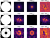 |
Fig. 1 Illustration of the preprocessing step of the focal plane data, i.e, the observation. For a non-coronagraphic system, the Airy pattern (perfect PSF) is subtracted from the PSF, and for the perfect coronagraph, the perfect PSF is simply a dark image (background). The images are then flattened with the cubic root. |
4 Policy optimization for NCPA
This section describes the control algorithm and optimization procedures for both the dynamics pω(st, at) and the policy πξ(at|st). The central concept is to train a dynamics model capable of predicting the next focal plane image – referred to as the observation – based on prior images (observations) and the applied DM commands. This learned model is then used to improve the control policy. The algorithm proceeds iteratively through three steps:
Running the policy model: the policy runs NCPA control loop for T time steps (a single episode).
Improving the dynamics model: the dynamics model is optimized using a supervised learning objective, Eq. (12).
Improving the policy model: the policy is optimized by using the dynamics model; see Eq. (14).
During each iteration (steps 1–3), the algorithm gathers one episode of data – consisting of 20 consecutive focal plane images (time steps) and the corresponding DM commands – by executing the policy within the NCPA control loop. The collected observations and actions are stored, and the policy and dynamics models are then updated using gradient-based optimization on all accumulated data. Our experiments (Sect. 5) show that PO4NCPA converges within around 10–15 time steps for each test case; hence, an episode length of 20 time steps is a good value for learning the full range of needed actions. The following subsections describe the observation representation, the NN architectures of the dynamics and policy, and the optimization procedure.
4.1 Focal plane wavefront control as a Markov decision process
The environment in which the RL algorithm operates consists of the electric field of the incoming light, the optics, the potential coronagraph, the phase modification due to NCPA errors, and the DM. The RL algorithm interacts with the environment by giving residual commands to the DM. Together, these form an MDP, where the next state depends only on the previous state (previous DM position, electric field, and NCPA error) and the applied DM command. However, we do not directly observe the electric field; we measure it with a science camera, with or without a coronagraph, i.e., we measure the intensity of the focal plane electric field (see Eqs. (3), (4), and (5)). As discussed before, the full electric field cannot be recovered from a single focal plane image (phase ambiguity). Hence, the focal plane image can only be considered as a partial observation of the underlying MDP. One way to resolve phase ambiguity in the observation is to include the previous focal plane image and the given differential DM command, that is, via sequential phase diversity (Gonsalves 2002).
Moreover, we modify the focal plane image to better suit NNs trained with stochastic gradient descent. In the case of noncoronagraphic PSFs and VVC with ELT pupil, a significant amount of light contributes to the diffraction pattern, noted as PSFideal (see the third column in Fig. 1). The focal plane intensity is very unevenly distributed, and the speckles resulting from optical aberrations closer to the center are up to several hundred times brighter than the speckles further away. Hence, we subtract the diffraction pattern and flatten the resulting image using a cubic root; the final observation is given by (see Fig. 1)
 (7)
(7)
Further discussion on this choice can be found in Sect. 6. Actions are defined as a vector of Zernike mode coefficients applied on top of the last full DM command:  . To prevent the algorithm from learning to steer the light outside the defined focal plane, the DM is numerically clipped to the maximum expected NCPA error, that is, each mode at three standard deviations of the NCPA spectrum (this parameter is just a crude limit for the clipping, and the algorithm was not sensitive to the exact value). The DM command (action vector) is also normalized with this value. Let
  be the vector of the expected maximum values. The residual command sent to the DM is then given by
 (8)
(8)
Now we define the state of the environment (as MDP) by
 (9)
(9)
This formulation follows approximately Markovian statistics (previous image and command providing the needed phase diversity), that is, the next state depends (and can be inferred) only on the information from the last state and the given action at.
For a state-action pair, the reward was chosen as a negative Euclidean norm between the expected ideal, non-distorted PSF, and observation, that is,
 (10)
(10)
where  is a distribution obtained from
  (probabilistic transition dynamics). The reward here is calculated for the full focal plane image. It could also be calculated on photometric apertures tailored to the application, for example, a one-sided dark hole. Moreover, because the best reward is achieved when a diffraction-limited PSF is observed, the RL algorithm will never try to “apodize” the PSF. In particular, when digging deep, dark holes, the reward (or the ideal PSF subtraction in the observation) must be modified to enable RL to go beyond the perfect PSF via apodization.
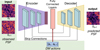 |
Fig. 2 Dynamics model NN design. Trained on closed-loop data (science camera images and residual commands), the dynamics model learns to simulate the optical path of the light. Highlighted in green are the inputs to the NN. |
4.2 The dynamics model
The state information includes two different data tensor shapes. The focal plane images are 2D, whereas the DM commands are vectors of Zernike modes. We designed the dynamics model to account for the different shapes. The dynamics model has two input channels: one for focal plane images and one for DM commands. The image channel consists of multiple convolutional layers, a flattening operation, and a fully connected layer. The DM command channel concatenates the vector inputs with the output of the images channel vector. The concatenated vector is then propagated through one fully connected layer, which is subsequently reshaped into a 3D tensor. The 3D tensor is then propagated through multiple convolutional layers to form an image representing the next focal plane. The convolutional layers have skip connections to the previous layers (see Fig. 2). This deterministic dynamics model  predicts the next state st+1 based on the current state and action. The model parameters ω – representing the neural network’s weights and biases – are learned by executing the policy π in the environment, that is, by using the policy to control the AO system, collecting tuples (st, at, st+1) in a dataset 𝒟, and minimizing the loss function J, the root mean square error between the predicted and actual next states (overload notation for clarity)
 (11)
(11)
where ot+1 is obtained from the state st+1 and ôt+1 is the observation predicted by  .
.
In focal plane control, the dynamics model must be accurate across a wide range of input strengths. The mean squared error (Eq. (11)) takes the square of the absolute error, which effectively causes the optimizer to focus more on wavefronts with relatively larger input values (large wavefront errors, i.e., small Strehl). As a remedy, we followed the approach of Landman & Haffert (2020) and introduced a relative loss function Jrelative for dynamics optimization, that is, we opted to weigh the mean squared error by the square of the RMSE of the true (label) observation
 (12)
(12)
where ⟨·⟩ denotes the mean over a sample batch. The ϵ is introduced to avoid divergence for very small input RMSE (≈ 10−7). The optimization was performed using the Adam algorithm (Kingma & Ba 2014).
It is well established that model-based RL can suffer poor performance due to overfitting of the dynamics model, which can be overly exploited during control tasks such as planning or policy optimization, particularly in the early stages of training (Nagabandi et al. 2018). To mitigate this issue, we used an ensemble of dynamics models, where each model was trained on a different bootstrap dataset, that is, a randomly sampled subset of the collected observations. As a result, each model in the ensemble is exposed to a distinct portion of the training data, leading to diverse neural network approximations. During policy training, predictions from all ensemble members are averaged (see lines 13 and 15 of Algorithm 1). For further discussion on the use of ensemble models in this context, see Chua et al. (2018).
4.3 The policy model
Similarly to the dynamics model, the policy model πξ(st) also has image and vector inputs. The image inputs are again propagated through convolutional layers, then reshaped into a vector and propagated through some fully connected layers, with the final layer forming the vector output of Zernike coefficients, the action. The previous action (phase diversity action) is concatenated to the first fully connected layer (see Fig. 3). The policy model parameters are then optimized using the dynamics model. More precisely, we use the dynamics model to generate trajectories of length H (called the planning horizon) starting from states in the data set, with the policy serving as the controller. We then collect rewards and backpropagate through the models to obtain policy gradients and optimize the policy parameters ξ.
We define
 (13)
(13)
where ôt+1 is obtained from  . This leads to the approximate policy optimization problem: we approximate Eq. (1), with learned dynamics and a cropped horizon, that is,
 (14)
(14)
where H is the so-called planning horizon and

To avoid policy optimization from getting stuck in a local minimum, we randomize the horizon length by randomly sampling an integer between hmin and hmax. The algorithm 1 presents the complete training procedure for the dynamics model and the policy. The while loop on line 3 cycles through episodes until the performance criteria (i.e., the cumulative reward over episode) converge. Lines 6–16 implement a policy update through policy optimization.
1: Initialize policy and dynamics model parameters ξ and ω randomly and set ensemble dynamics size n
2: Initialize gradient iteration length K, batch size B < |𝒟| and planning horizon H limits
3: while not episode reward converged do
4: Generate samples {st+1, st, at} by running policy πξ(at|st) for T timesteps (an episode) and append to 𝒟
5: Fit dynamics by minimizing Eq. (12) w.r.t ω using Adam
6: for iteration k = 1 to K do
7: Sample a mini batch of B < |𝒟| states {sτ} from 𝒟
8: for each sτ in the mini batch do
9: Set 
10: Draw H from (hmin, hmax)
11: for t = 1 to H do
12: Predict at = πξ(st)
13: Predict 
14: Calculate 
15: Ensemble avg next state 
16: end for
17: end for
18: Update ξ by taking a gradient step according to  with Adam.
19: end for
20: end while
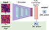 |
Fig. 3 Policy model NN design. In the control loop, the image inputs (ot, and ot−1) are focal plane images from the science camera, and while training, the future inputs (Algorithm 1 line 11, t = 2, 3, · · · H) are predicted (i.e., simulated) by the dynamics model. |
5 Numerical experiments
5.1 Simulation description
This section evaluates the performance of PO4NCPA using numerical simulations. First, we demonstrate the method’s performance against both static and dynamic NCPA errors, considering two focal planes: one with a perfect (i.e., ideal) coronagraph (PC) and the other without (i.e., standard imaging, SI). Second, we demonstrate the performance of PO4NCPA on a possible use case for the algorithm: WV seeing control for ELT-METIS equipped with a VVC. The examples presented here have been chosen to demonstrate the method’s versatility and performance, which is agnostic to imaging conditions (standard imaging or any coronagraphy) and fast enough to cope with dynamic NCPA, while keeping the results section compact.
We used the HCIPy (Por et al. 2018) package to simulate telescopes, NCPA aberrations, the DM, and coronagraphs (PC and VVC). For the first demonstration (PC or SI), we simulated a 39.3-meter telescope with a circular pupil and no central obstruction, while for the VVC demonstration, we used the latest ELT pupil description released by ESO, which includes one thicker spider arm (386 mm instead of 202 mm) due to the presence of the ELT primary mirror crane (see Fig. 1). We note that this thicker spider effectively breaks the symmetry of the input pupil, which is expected to give this simulation setup an edge in lifting the ambiguity for even Zernike modes. The DM was modeled as a device that applies a command vector comprising Zernike coefficients. The experiments were run with 55 modes (a choice discussed in Sect. 6). The focal plane is sampled with three pixels per full width at half maximum (FWHM), and the image was cropped to contain 5.5 λ/D. These parameters yielded a 33 × 33 pixel focal plane image that covered well the control radius of the DM (55 Zernike modes). We assumed a frame rate of 10 Hz for the correction of dynamic NCPA (as recommended for WV seeing by Orban de Xivry et al. 2024), and no AO residual wavefront error.
To keep the results section clear and enable easy comparison between PO4NCPA’s static and dynamic NCPA performance, we used the same spatial NCPA spectrum across all experiments. We used the WV seeing spectrum derived by Orban de Xivry et al. (2024) – the NCPA phase error screens are drawn from the Kolmogorov spectrum with r0 of 95 meters at 11 μm and an outer scale of 500 meters. The resulting median RMSE of these phase screens is 286 nm. For the dynamics NCPA cases, we propagated a single layer according to Taylor’s frozen flow hypothesis at a wind speed of 10 m/s (corresponding to a coherence time of 2.9 s). We subtracted the piston and tip-tilt modes from all of the phase screens; that is, we assumed that the considered instruments have ways to deal with PSF centering, for example, a reflective Lyot stop (with high-speed control-loop, Singh et al. 2014) or QACITS (Huby et al. 2015) for coronagraphic systems, and normal centroiding for SI. Again, for clarity, all experiments were run at a wavelength of 11 μm (N-band). We note here that the median RMSE (286 nm on the N-Band, without piston and tip-tilt) corresponds to 42 nm at 1.65 μm (H-band) in the resulting PSFs. The aberration strength relates to typical NCPAs encountered in NIR and visible HCI instruments such as SPHERE (around 50 nm, Vigan et al. 2019) and MagAO-X (less than 30 nm, Van Gorkom et al. 2021).
The PO4NCPA was tested in the following five experiments representing different environments, using the exact same hyperparameters (see PO4NCPA parameters in Table 1):
Circular pupil and standard imaging (SI)
Static NCPA: we drew a static NCPA error and let the algorithm optimize the focal plane image, that is, maximize the reward defined in Eq. (13) by controlling the DM.
Dynamic NCPA: we simulated an evolving NCPA pattern, resembling the expected WV seeing for the ELT/METIS instrument (Absil et al. 2022). Again, the algorithm aims to maximize the reward by controlling the DM.
Circular pupil and perfect coronagraph (PC)
Static NCPA: same as item 1 above.
Dynamic NCPA: same as item 2 above.
ELT pupil and VVC and noise
Dynamic NCPA: as a possible use-case, we simulated an ELT/METIS-like system with ELT aperture, dynamic NCPA (WV seeing), photon and background noise, and VVC.
We compare PO4NCPA with three references:
Fitting error: perfect phase correction, that is, the NCPA phase error projected onto the DM Zernike modes, leaving only the high-order fitting errors.
Fitting error and delay error: for the dynamics NCPA case, we couple the perfect phase correction above with a 1-step delay integrator with a gain of 0.8.
Open loop: no phase correction.
We used two types of performance metrics: PSF-related (Strehl ratio, PSF contrast, residual light after the coronagraph) and pupil-plane wavefront error-related (residual RMSE and modal RMSE). The PO4NCPA optimizes PSF-related performance, and wavefront-related performance is a consequence of PSF optimization. We note that these performance metrics do not always align with one another.
Simulations parameters.
5.2 Circular pupil with SI and PC results
5.2.1 Training
Dynamic and static NCPA codes are trained with the same strategy. The episode length was set to 20 steps. The first 4000 are run with random commands (drawn from a Gaussian distribution with a standard deviation of 0.2 times the total DM response). This phase is called the warm-up.
For static NCPA, a new phase screen is generated at the beginning of each episode and the DM is flattened. In dynamic NCPA cases, the phase screen is propagated at every time step, and the DM is flattened only during the first 40k episodes to avoid starting episodes at a saturated DM position. After the first 40k episodes, each subsequent episode begins from the end position of the previous one, simulating a closed-loop control system in which the new model is continuously updated.
After each episode, excluding the warm-up, the dynamic codes are trained for eight gradient steps, and the policy for five gradient steps. The training procedure was continued until the performance (cumulative episode reward) converged. We examined the convergence speed of the method by plotting the cumulative reward (a measure of the distance from the perfect PSF) at the end of each episode (see Fig. 4). All cases converge by 50k episodes at the latest. The end of the warm-up phase (4k) and the end of resetting the DM after each episode (at 40k in the dynamic cases) are clearly visible in the plots. At 40k in the dynamic cases, we see some instability at first because PO4NCPA encounters new types of starting positions (not only open-loop WV seeing), but after some episodes, we observe improved performance since PO4NCPA starts from smaller residuals. Furthermore, with the given hyperparameters, the training procedure always converged, producing nearly identical training curves (which is not trivial in RL in general).
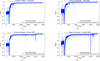 |
Fig. 4 Training plots of PO4NCPA on circular pupil with SI and PC. Here we plot the negative cumulative reward (loss) after each episode in the training circle. The light blue curve shows the raw negative reward, and the dark blue shows the smoothed value (moving average). For the dynamic case (c, d), the DM is flattened only at the start of the episode for the first 40k episodes to prevent saturation. Afterward, each episode starts from the previous endpoint, thereby mimicking a continuously updated closed-loop control system. Hence, the bigger episode reward after that. |
5.2.2 Performance on static NCPA
After the training procedure, we ran 500 episodes with the final policy. Each episode started with a randomly sampled NCPA phase screen and flat DM. We then let the policy run for 20 steps and recorded data at each time step for each episode. The results are visualized in two ways.
First, we order the episodes by the final reward (Eq. (13)) at the last step (step #20). We then plotted the temporal evolution of the negative reward (correlated with the contrast of PSF sharpness) for the best, median, and worst episodes; see Figs. 5a and 5b. We also plotted the corresponding wavefront RMSE within the control radius (RMSE-fitting RMSE) during these episodes in Figs. 5c and 5d. We note that the reward is the quantity that the algorithm tries to maximize, and the small RMSE is only a consequence of this process. In both PC and SI cases, convergence occurs in around ten time steps. Without a coronagraph, PO4NCPA achieves a final reward (relative to Strehl) close (but slightly worse) to the reward of fitting error (the colored PO4NCPA lines coincide with black and gray fitting error lines). The corresponding RMSE errors are 9 nm for the best, 17 nm for the median, and 26 nm for the worst. In the case of a PC, PO4NCPA achieves equal (worst episode) or better (median and best) reward than the fitting error (Fig. 5b), meaning that PO4NCPA learns to find a combination of commands that removes more light from the focal plane than the fitting of DM modes – reward is calculated in the whole focal plane image, that is, not only inside the dark hole. The corresponding RMSE are 2 nm (best), 4 nm (median), and 5 nm (worst).
Second, we calculate the mean PSF radial average over the last time step across the 500 different episodes and compare it with the integrator and open-loop (see Fig. 6). In the SI case, PO4NCPA learns to sharpen the slightly distorted PSF (Strehl 95.6%) to the fitting error limit, resulting in an average Strehl ratio of 99.4%. In contrast, the fitting error Strehl was 99.6%. In the PC case, PO4NCPA obtains better contrast from 2.7–4.5 λ/D than the fitting error, while the fitting error is better at 0–2.7 λ/D. We note here that PO4NCPA tries to maximize the reward in the whole focal plane (see Sect. 4.3). The total fitting error flux is 0.104%, and PO4NCPA is slightly better at 0.102%, which means that PO4NCPA learns to compromise the contrast near the PSF core to gain contrast farther away by pushing light outside of the field of view (5.5 λ/D).
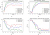 |
Fig. 5 PO4NCPA convergence on circular pupil with SI (left) and PC (right) in the case of static NCPA. Top row: reward on time steps. PO4NCPA episodes are shown in green (best), blue (median), red (worst), while black and gray lines correspond to fitting error rewards. Bottom row: PO4NCPA residual wavefront RMSE (inside the control region) over the same episodes (fitting error is always zero). |
5.2.3 Dynamic NCPA
For dynamic NCPA errors, after the training procedure, we ran the final policy on a single longer episode. We started with a randomly sampled NCPA phase screen and flat DM, and then let the policy control the DM for 5000 time steps (i.e, 500s) under dynamic NCPA perturbations. We compared PO4NCPA against the fitting error, the fitting error plus the time delay error, and the open-loop (no correction).
Again, the results are visualized in three ways. First, we plot a randomly sampled 100-step sequence of RMS errors (see Fig. 7) for the fitting error (dashed black), the fitting error plus the time delay error (dot-dashed gray), and PO4NCPA (blue). Here, the PO4NCPA RMS error follows the “fitting error plus time-delay error” pattern, suggesting that it provides only minimal prediction but can reconstruct the modal coefficients close to the level of perfect reconstruction.
Second, we plot the modal RMS over the time series to understand how the method behaves with respect to modes; see Fig. 8. In the SI case, we can clearly see the difference between even modes (sign ambiguity) and odd modes. For odd modes, we observe a factor of 9 improvement over lower-order modes, suggesting that PO4NCPA learns to predict them. For even modes, performance is diminished, but PO4NCPA still achieves a level of time-delay error on low-order modes, whereas high-order modes are only slightly corrected. With the PC, there is no difference between even and odd modes, as expected. Instead, we observe that PO4NCPA residuals are smaller only for lower-order modes (1–7), suggesting predictive capability on these modes. We also note that the modal RMS is not the quantity that PO4NCPA tries to minimize; this behavior arises only as a consequence of minimizing the reward function (PSF sharpness and/or contrast).
Third, Fig. 9 plots the long-exposure PSFs (over the entire time sequence, excluding the first 20 steps) and their radial averages. For SI, the PO4NCPA PSF closely follows the fitting-error PSF, with no notable difference. The achieved Strehl ratio is, respectively, of 95.4% (open loop), 99.6% (fitting error plus delay error), and 99.4% (PO4NCPA). The PO4NCPA raw contrast curve closely follows the fitting error plus delay error curve. We also observe that PO4NCPA obtains slightly better contrast at 0–1.8 λ/D, while the fitting error plus delay error is otherwise slightly better. The total amount of light on the focal plane is, respectively, 2.75% (open loop), 0.104% (fitting error), 0.257% (fitting error plus delay error), and 0.275% (PO4NCPA).
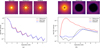 |
Fig. 6 Circular pupil PSF sharpness and raw contrast with static NCPA for (a) standard imaging and (b) perfect coronagraph cases. Here, we take the average (over 500 episodes) of the last PSF frame and plot the resulting PSF and radial average divided by the peak intensity. |
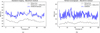 |
Fig. 7 A 100 time-step window during the long exposure dynamic NCPA, showing the wavefront RMS error as a function of time steps. (a) Standard imaging and (b) perfect coronagraph cases. |
5.2.4 Robustness to larger wavefront errors
The NCPA errors (from the WV seeing spectrum) simulated in the previous subsections are rather small and have a small impact on the Strehl ratio. A natural follow-up question is whether PO4NCPA can handle larger wavefront errors. This way it could be used, for example, to dynamically correct the low-wind effect or even drive smaller AO systems without WFS. To this end, we ran an experiment using SI plus dynamic NCPA, with the turbulence strength modified by tuning the Fried parameter. We started from the previously defined value of 95 m in the N-band and lowered it until PO4NCPA no longer performed with the same training procedure and hyperparameter set as before. This time, we did not remove the tip-and-tilt modes; hence, no external centering was needed. Each seeing case (i.e., different r0) is trained separately from the beginning. We ran the training procedure and collected the Strehl ratio for long exposure (5000 frames) for five different r0 values: 95 m, 30 m, 20 m, 15 m, and 10 m. These values resulted in median piston-removed RMS values of 520 nm, 1336 nm, 1902 nm, 2412 nm, and 3377 nm. The latter corresponds to almost 2 rad RMS for 11µm.
We compare PO4NCPA performance across different wavefront error levels with the previously introduced fitting error plus delay error and open-loop (i.e., no correction). The training procedure converged for Fried parameters (r0) of 95 m, 30 m, and 20 m, and the long exposure Strehl ratio of the final policy closely follows the fitting error plus delay error (see Fig. 10). The PO4NCPA training did not converge for r0 = 15 m and r0 = 10 m; instead, it was stuck at an undesired solution (presumably a local minimum of the policy training objective), resulting in poor final performance. However, we also ran the long exposure with controller (i.e., policy) trained on r0 = 20 m with r0 = 15 m and r0 = 10 m; this version of PO4NCPA managed to control the r0 = 15 m case decently (Strehl 85%, see the green line in Fig. 10), and also managed to control wavefront errors sometimes for r0 = 10 m, but was unstable to obtain improved long exposure Strehl ratio.
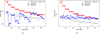 |
Fig. 8 RMS per mode over the long episode with dynamic NCPA for (a) standard imaging and (b) perfect coronagraph cases. |
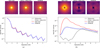 |
Fig. 9 PSF sharpness and/or contrast with dynamic NCPA for (a) standard imaging and (b) perfect coronagraph cases. |
5.3 ELT pupil with VVC and noise results
As a possible use-case demonstration, we simulated an ELT/METIS-like system with dynamic NCPA. Compared to the other dynamic NCPA cases, the METIS case uses the ELT pupil, the VVC instead of a PC, and adds photon and strong background noise, typical for ground-based N-band observations (see Table 1).
For the METIS WV seeing control, we ran the same training procedure, followed by a single 5000-step episode with WV seeing (dynamic NCPA). We only recorded the long-exposure PSF (after training) and calculated the contrast (see Fig. 11). We subtract the diffraction pattern (ideal PSF) from the PSFs for a better comparison. We again compare the PO4NCPA against the fitting error, the fitting error plus time-delay error, and the open-loop. Compared to open-loop, PO4NCPA yields an improvement of up to a factor of 40 at 1.5 λ/D and around a factor of 10 at 1.6–3 λ/D. Similarly to the PC experiment, PO4NCPA delivers contrast close to the fitting error plus delay error, the latter yielding slightly better overall performance.
6 Conclusion and future work
We introduced a new focal plane wavefront control algorithm, PO4NCPA. We showed that, when implemented well, it provides near-optimal control, as measured by the reward function (related to the Strehl ratio or post-coronagraphic residual flux), across various NCPA error scenarios. The method makes minimal assumptions about the optical design and can therefore be applied to different optical paths without altering the algorithm. The PO4NCPA training phase takes relatively long (∼24 h including the time spent on the numerical simulation) on standard off-the-shelf graphics processing unit and computer. However, the trained policy model (i.e., controller) is fast to use (inference time <1 ms).
The method was tested in a numerical simulation that demonstrated robust promising performance for static and dynamic NCPA error compensation. In the static NCPA case, PO4NCPA achieves near-optimal performance (in terms of reward). With a perfect coronagraph, PO4NCPA removes more light from the focal plane than the modal least-squares projection, and without a coronagraph, PO4NCPA achieves nearly perfect Strehl. In the dynamic NCPA case, PO4NCPA reaches the performance of the modal least-squares projection combined with a 1-step delay integrator in terms of reward. In terms of wavefront RMS, the performance is farther from the reference method, especially for high-order modes. Additionally, PO4NCPA proved capable of correcting larger wavefront errors. In the current training setup, the system remained stable up to a median piston-removed RMS of approximately 1902 nm (FP-WFS at 11 µm, corresponding to an open-loop Strehl of about 30%). The learned policy could even partially correct beyond this range, suggesting that, with an optimized learning strategy, the method could adapt to increasingly severe wavefront errors.
In principle, PO4NCPA can perform predictive control in the dynamic NCPA case. Examination of the modal rejection of dynamic SI in Fig. 8a indicates that unambiguous modes are corrected significantly more effectively than with the fitting error plus time-delay error. In contrast, performance in ambiguous modes is comparable to or worse than time delayed correction of fitting error plus time-delay error. This suggests that predictive correction is primarily effective for modes that are unambiguous on the focal plane. However, with a PC, we observe comparable behavior across all modes, since all modes are (to some extent) ambiguous (Fig. 8b). We attribute this difference to the requirement for phase diversity in the ambiguous modes. In dynamic NCPA cases, there is always a component of new errors (even with perfect prediction, e.g., Nousiainen et al. 2024b) for which PO4NCPA must first determine the correct phase sign before applying a correction, which delays the correction process. Consistent with this interpretation, most residual errors are observed along the direction of the wind (see Fig. 9b). These results suggest that the algorithm suits wavefront-sensorless AO (with or without a coronagraph), where the correction speed is set by the focal-plane camera’s frame rate. However, with the current setup, adding more DM modes did not improve performance – PO4NCPA remains limited to relatively low-order corrections.
Our results show that PO4NCPA also works with the ELT pupil, a vortex coronagraph, and photon and background noise without any modifications to the algorithm. A more thorough analysis of the error terms in these cases is left for future work. As a caveat, the algorithm – like most deep reinforcement learning methods – is somewhat sensitive to hyperparameter choices (e.g., network depth, learning rate, and related settings). Furthermore, deep learning-based control strategies are difficult to analyze theoretically and formal stability guarantees cannot currently be established.
An obvious line of future work is to study further the METIS VVC WV seeing case. For example, we can perform more accurate numerical simulations that include AO residuals, LWE, intensity variations, and static NCPAs. We will also explore how pupil asymmetries (Orban de Xivry et al. 2024) can help improve the control of even modes. Another interesting direction for future work is the design of a reward function for corona-graphic AO. Here, the reward was defined in the whole focal plane. We could consider defining a smaller one-sided region to dig a deeper dark hole within the area of interest, as well as removing the diffraction pattern subtraction (see Fig. 1) to allow PO4NCPA to apodize beyond the diffraction pattern.
In addition, moving from numerical simulations to laboratory and on-sky testing requires additional consideration and research. Most prominently, given the method’s long training time, it is not feasible to train it on-sky; therefore, a suitable training strategy needs to be studied. For example, first pretraining on a numerical simulation, then fine-tuning with the actual system during the daytime using an internal light source, and finally online training in parallel with closed-loop operation, enabling online adaptation to changing conditions.
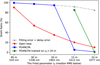 |
Fig. 10 PO4NCPA performance compared against “Fitting error + delay error” on larger dynamic wavefront errors in the standard imaging case. The dashed gray line is the “Fitting error + delay error”, the red line is the open-loop (i.e., no-correction) Strehl, the blue line is the PO4NCPA trained on the given r0, and the green line is the PO4NCPA trained on r0 = 20 m applied to r0 = 15 m and 10 m. |
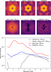 |
Fig. 11 Raw “residual” PSF contrast for ELT-METIS. Upper row: recorded PSF. Middle row: recorded PSFs with diffraction patterns (ideal PSF) subtracted. Lower row: Azimuthal average of the subtracted PSFs (i.e., “Raw residual PSF contras”). |
References
- Absil, O., Delacroix, C., Orban de Xivry, G., et al. 2022, in Proc. SPIE Conf., 12185, SPIE, 298 [Google Scholar]
- Absil, O., Mawet, D., Karlsson, M., et al. 2016, Proc. SPIE Conf., 9908, 99080Q [Google Scholar]
- Angel, J. R. P., Wizinowich, P., Lloyd-Hart, M., & Sandler, D. 1990, Nature, 348, 221 [NASA ADS] [CrossRef] [Google Scholar]
- Bos, S. P., Vievard, S., Wilby, M. J., et al. 2020, A&A, 639, A52 [NASA ADS] [CrossRef] [EDP Sciences] [Google Scholar]
- Bottom, M., Walker, S. A. U., Cunnyngham, I., Guthery, C. E., & Delorme, J.-R. 2023, in AO4ELT7, 125 [Google Scholar]
- Brandl, B., Absil, O., Feldt, M., et al. 2024, in Proc. SPIE, 13096 [Google Scholar]
- Cavarroc, C., Boccaletti, A., Baudoz, P., Fusco, T., & Rouan, D. 2006, A&A, 447, 397 [NASA ADS] [CrossRef] [EDP Sciences] [Google Scholar]
- Chua, K., Calandra, R., McAllister, R., & Levine, S. 2018, in NeurIPS, 4754 [Google Scholar]
- Currie, T., Biller, B., Lagrange, A., et al. 2023, in Astronomical Society of the Pacific Conference Series, 534, Protostars and Planets VII, eds. S. Inutsuka, Y. Aikawa, T. Muto, K. Tomida, & M. Tamura, 799 [NASA ADS] [Google Scholar]
- Deisenroth, M., & Rasmussen, C. E. 2011, in ICML-11, Citeseer, 465 [Google Scholar]
- Dinis, I., Wildi, F., Ségransan, D., et al. 2024, in Proc. SPIE Conf., 13097, SPIE, 1876 [Google Scholar]
- Durech, E., Newberry, W., Franke, J., & Sarunic, M. V. 2021, Biomed. Opt. Express, 12, 5423 [Google Scholar]
- Give’on, A., Kern, B., Shaklan, S., Moody, D. C., & Pueyo, L. 2007, in Proc. SPIE Conf., 6691, SPIE, 63 [Google Scholar]
- Give’on, A., Kern, B. D., & Shaklan, S. 2011, in Proc. SPIE Conf., 8151, SPIE, 376 [Google Scholar]
- Gonsalves, R. A. 1982, Opt. Eng., 21, 829 [NASA ADS] [CrossRef] [Google Scholar]
- Gonsalves, R. A. 2002, in ESO Conf. and Works. Proc., 58, eds. E. Vernet, R. Ragazzoni, S. Esposito, & N. Hubin, 121 [Google Scholar]
- Gonsalves, R. A. 2010, Frontiers in Optics, Optica Publishing Group, FWV1 Gutierrez, Y., Mazoyer, J., Mugnier, L. M., Herscovici-Schiller, O., & Abeloos, B. 2024, Opt. Express, 32, 31247 [Google Scholar]
- Guyon, O. 2005, ApJ, 629, 592 [NASA ADS] [CrossRef] [Google Scholar]
- Guyon, O. 2018, ARA&A, 56, 315 [Google Scholar]
- Guyon, O., & Males, J. 2017, arXiv e-prints [arXiv:1707.00570] [Google Scholar]
- Guyon, O., Matsuo, T., & Angel, R. 2009, ApJ, 693, 75 [NASA ADS] [CrossRef] [Google Scholar]
- Haffert, S., Males, J., Ahn, K., et al. 2023, A&A, 673, A28 [NASA ADS] [CrossRef] [EDP Sciences] [Google Scholar]
- Huby, E., Baudoz, P., Mawet, D., & Absil, O. 2015, A&A, 584, A74 [NASA ADS] [CrossRef] [EDP Sciences] [Google Scholar]
- Jovanovic, N., Martinache, F., Guyon, O., et al. 2015, PASP, 127, 890 [NASA ADS] [CrossRef] [Google Scholar]
- Ke, H., Xu, B., Xu, Z., et al. 2019, Optik, 178, 785 [NASA ADS] [CrossRef] [Google Scholar]
- Keller, C. U., Korkiakoski, V., Doelman, N., et al. 2012, in Proc. SPIE Conf., 8447, SPIE, 749 [Google Scholar]
- Kingma, D. P., & Ba, J. 2014, arXiv e-prints [arXiv:1412.6980] [Google Scholar]
- Korkiakoski, V., Keller, C. U., Doelman, N., et al. 2014, Appl. Opt., 53, 4565 [NASA ADS] [CrossRef] [Google Scholar]
- Kuznetsov, A., Neichel, B., Oberti, S., & Fusco, T. 2023, in AO4ELT [Google Scholar]
- Landman, R., & Haffert, S. Y. 2020, Opt. Express, 28, 16644 [NASA ADS] [CrossRef] [Google Scholar]
- Landman, R., Haffert, S., Males, J., et al. 2024, A&A, 684, A114 [NASA ADS] [CrossRef] [EDP Sciences] [Google Scholar]
- Landman, R., Haffert, S., Long, J., et al. 2025, A&A, 696, L1 [NASA ADS] [CrossRef] [EDP Sciences] [Google Scholar]
- Macintosh, B. A., Graham, J. R., Palmer, D.W., et al. 2008, in Proc. SPIE Conf., 7015, SPIE, 315 [Google Scholar]
- Males, J. R., & Guyon, O. 2018, JATIS, 4, 019001 [Google Scholar]
- Marois, C., Racine, R., Doyon, R., Lafrenière, D., & Nadeau, D. 2004, ApJ, 615, L61 [NASA ADS] [CrossRef] [Google Scholar]
- Marois, C., Lafrenière, D., Doyon, R., Macintosh, B., & Nadeau, D. 2006, ApJ, 641, 556 [Google Scholar]
- Martinache, F. 2013, PASP, 125, 422 [NASA ADS] [CrossRef] [Google Scholar]
- Mawet, D., Riaud, P., Absil, O., & Surdej, J. 2005, ApJ, 633, 1191 [Google Scholar]
- Milli, J., Kasper, M., Bourget, P., et al. 2018, in Proc. SPIE Conf., 10703, SPIE, 752 [Google Scholar]
- Nagabandi, A., Kahn, G., Fearing, R. S., & Levine, S. 2018, in 2018 IEEE International Conference on Robotics and Automation (ICRA), IEEE, 7559 [Google Scholar]
- Nousiainen, J., Rajani, C., Kasper, M., & Helin, T. 2021, Opt. Express, 29, 15327 [NASA ADS] [CrossRef] [Google Scholar]
- Nousiainen, J., Rajani, C., Kasper, M., et al. 2022, A&A, 664, A71 [NASA ADS] [CrossRef] [EDP Sciences] [Google Scholar]
- Nousiainen, J., Engler, B., Kasper, M., et al. 2024a, JATIS, 10, 019001 [Google Scholar]
- Nousiainen, J., Puska, J.-P., Helin, T., Hyvönen, N., & Kasper, M. 2024b, JATIS, 10, 039001 [Google Scholar]
- Orban de Xivry, G., & Absil, O. 2024, in Proc. SPIE Conf., 13097, SPIE, 982 [Google Scholar]
- Orban de Xivry, G., Absil, O., Delacroix, C., et al. 2024, in Proc. SPIE Conf., 13097, SPIE, 974 [Google Scholar]
- Orban de Xivry, G., Quesnel, M., Vanberg, P. O., Absil, O., & Louppe, G. 2021, MNRAS, 505, 5702 [NASA ADS] [CrossRef] [Google Scholar]
- Otten, G. P. P. L., Vigan, A., Muslimov, E., et al. 2021, A&A, 646, A150 [EDP Sciences] [Google Scholar]
- Parvizi, P., Zou, R., Bellinger, C., Cheriton, R., & Spinello, D. 2023, Photonics, 10 [Google Scholar]
- Por, E. H., Haffert, S. Y., Radhakrishnan, V. M., et al. 2018, in Proc. SPIE Conf., 10703, SPIE, 1112 [Google Scholar]
- Pou, B., Smith, J., Quinones, E., Martin, M., & Gratadour, D. 2024, Opt. Express, 32, 37011 [Google Scholar]
- Quesnel, M., Orban de Xivry, G., Absil, O., & Louppe, G. 2022, in Proc. SPIE Conf., 12185, SPIE, 982 [Google Scholar]
- Quesnel, M., Orban de Xivry, G., Louppe, G., & Absil, O. 2022, A&A, 668, A36 [NASA ADS] [CrossRef] [EDP Sciences] [Google Scholar]
- Riaud, P., Mawet, D., & Magette, A. 2012, A&A, 545, A151 [NASA ADS] [CrossRef] [EDP Sciences] [Google Scholar]
- Ruffio, J.-B., & Kasper, M. 2022, arXiv e-prints [arXiv:2211.00775] [Google Scholar]
- Singh, G., Martinache, F., Baudoz, P., et al. 2014, PASP, 126, 586 [Google Scholar]
- Skaf, N., Guyon, O., Gendron, É., et al. 2022, A&A, 659, A170 [NASA ADS] [CrossRef] [EDP Sciences] [Google Scholar]
- Snellen, I., de Kok, R., Birkby, J. L., et al. 2015, A&A, 576, A59 [NASA ADS] [CrossRef] [EDP Sciences] [Google Scholar]
- Terreri, A., Pedichini, F., Del Moro, D., et al. 2022, A&A, 666, A70 [NASA ADS] [CrossRef] [EDP Sciences] [Google Scholar]
- Van Gorkom, K., Males, J. R., Close, L. M., et al. 2021, JATIS, 7, 039001 [Google Scholar]
- van Kooten, M. A., Jensen-Clem, R., Cetre, S., et al. 2022, JATIS, 8, 029006 [Google Scholar]
- Vigan, A., N’diaye, M., Dohlen, K., et al. 2019, A&A, 629, A11 [NASA ADS] [CrossRef] [EDP Sciences] [Google Scholar]
- Wong, A. P., Norris, B. R. M., Deo, V., et al. 2023, PASP, 135, 114501 [NASA ADS] [CrossRef] [Google Scholar]
Exoplanet Orbit Database: http://exoplanets.org/
The initial state s0 is sampled from an initial state distribution p0(s0).
This slightly thicker spider is due to the shadow of the ELT-M1 crane, located along one of the spiders.
All Tables
All Figures
|
Fig. 1 Illustration of the preprocessing step of the focal plane data, i.e, the observation. For a non-coronagraphic system, the Airy pattern (perfect PSF) is subtracted from the PSF, and for the perfect coronagraph, the perfect PSF is simply a dark image (background). The images are then flattened with the cubic root. |
| In the text | |
|
Fig. 2 Dynamics model NN design. Trained on closed-loop data (science camera images and residual commands), the dynamics model learns to simulate the optical path of the light. Highlighted in green are the inputs to the NN. |
| In the text | |
|
Fig. 3 Policy model NN design. In the control loop, the image inputs (ot, and ot−1) are focal plane images from the science camera, and while training, the future inputs (Algorithm 1 line 11, t = 2, 3, · · · H) are predicted (i.e., simulated) by the dynamics model. |
| In the text | |
|
Fig. 4 Training plots of PO4NCPA on circular pupil with SI and PC. Here we plot the negative cumulative reward (loss) after each episode in the training circle. The light blue curve shows the raw negative reward, and the dark blue shows the smoothed value (moving average). For the dynamic case (c, d), the DM is flattened only at the start of the episode for the first 40k episodes to prevent saturation. Afterward, each episode starts from the previous endpoint, thereby mimicking a continuously updated closed-loop control system. Hence, the bigger episode reward after that. |
| In the text | |
|
Fig. 5 PO4NCPA convergence on circular pupil with SI (left) and PC (right) in the case of static NCPA. Top row: reward on time steps. PO4NCPA episodes are shown in green (best), blue (median), red (worst), while black and gray lines correspond to fitting error rewards. Bottom row: PO4NCPA residual wavefront RMSE (inside the control region) over the same episodes (fitting error is always zero). |
| In the text | |
|
Fig. 6 Circular pupil PSF sharpness and raw contrast with static NCPA for (a) standard imaging and (b) perfect coronagraph cases. Here, we take the average (over 500 episodes) of the last PSF frame and plot the resulting PSF and radial average divided by the peak intensity. |
| In the text | |
|
Fig. 7 A 100 time-step window during the long exposure dynamic NCPA, showing the wavefront RMS error as a function of time steps. (a) Standard imaging and (b) perfect coronagraph cases. |
| In the text | |
|
Fig. 8 RMS per mode over the long episode with dynamic NCPA for (a) standard imaging and (b) perfect coronagraph cases. |
| In the text | |
|
Fig. 9 PSF sharpness and/or contrast with dynamic NCPA for (a) standard imaging and (b) perfect coronagraph cases. |
| In the text | |
|
Fig. 10 PO4NCPA performance compared against “Fitting error + delay error” on larger dynamic wavefront errors in the standard imaging case. The dashed gray line is the “Fitting error + delay error”, the red line is the open-loop (i.e., no-correction) Strehl, the blue line is the PO4NCPA trained on the given r0, and the green line is the PO4NCPA trained on r0 = 20 m applied to r0 = 15 m and 10 m. |
| In the text | |
|
Fig. 11 Raw “residual” PSF contrast for ELT-METIS. Upper row: recorded PSF. Middle row: recorded PSFs with diffraction patterns (ideal PSF) subtracted. Lower row: Azimuthal average of the subtracted PSFs (i.e., “Raw residual PSF contras”). |
| In the text | |
Current usage metrics show cumulative count of Article Views (full-text article views including HTML views, PDF and ePub downloads, according to the available data) and Abstracts Views on Vision4Press platform.
Data correspond to usage on the plateform after 2015. The current usage metrics is available 48-96 hours after online publication and is updated daily on week days.
Initial download of the metrics may take a while.