| Issue |
A&A
Volume 710, June 2026
|
|
|---|---|---|
| Article Number | A6 | |
| Number of page(s) | 10 | |
| Section | Numerical methods and codes | |
| DOI | https://doi.org/10.1051/0004-6361/202558120 | |
| Published online | 28 May 2026 | |
PDRs4All
XXI. Haute Couture: Spectral stitching of JWST MIRI-IFU cubes with matrix completion
1
Institut de Recherche en Astrophysique et Planétologie (IRAP), CNRS, CNES, Université de Toulouse,
France
2
Institut de Recherche en Informatique de Toulouse (IRIT), CNRS, Toulouse INP, Université de Toulouse,
France
3
Department of Physics & Astronomy, The University of Western Ontario,
Canada
4
Department of Astronomy, Graduate School of Science, The University of Tokyo,
Japan
★ Corresponding author. This email address is being protected from spambots. You need JavaScript enabled to view it.
Received:
14
November
2025
Accepted:
18
February
2026
Abstract
The Mid-Infrared Instrument (MIRI) is the imager and spectrograph covering wavelengths from 4.9 to 27.9 μm on board the James Webb Space Telescope (JWST). The MIRI Medium-Resolution Spectrometer (MRS) consists of four integral field units (IFU) and two wheels with three rotation settings, producing four spectral channels and three spectral sub-channels.. The 12 resulting spectral data cubes have different fields of view, spatial coverages, and spectral resolutions. The wavelength range of each cube partially overlaps with the neighboring bands, and the overlap regions typically show flux mismatches that have to be corrected by spectral stitching methods. The aim of stitching methods is to produce a single data cube incorporating the data of the individual sub-channels, which requires matching the spatial resolution and the flux discrepancies. We present Haute Couture, a novel stitching algorithm that uses nonnegative matrix factorization to perform a matrix completion, where the available MRS data cubes are treated as 12 sub-matrices of a larger incomplete matrix. Prior to matrix completion, we also introduced a novel preprocessing method to homogenize the global intensities of the 12 cubes. Our preprocessing consists of jointly optimizing a set of global scale parameters that maximize the fit between the cubes where spectral overlap occurs. We applied our novel stitching method to JWST data obtained as part of the PDRs4All observing program of the Orion Bar and produced a uniform cube reconstructed with the best spatial resolution over the full range of wavelengths.
Key words: methods: data analysis / methods: numerical / techniques: image processing
© The Authors 2026
 Open Access article, published by EDP Sciences, under the terms of the Creative Commons Attribution License (https://creativecommons.org/licenses/by/4.0), which permits unrestricted use, distribution, and reproduction in any medium, provided the original work is properly cited.
This article is published in open access under the Subscribe to Open model. This email address is being protected from spambots. You need JavaScript enabled to view it. to support open access publication.
1 Introduction
The James Webb Space Telescope (JWST; Gardner et al. 2006) is an infrared telescope launched in 2021. Four instruments are on board: the Mid-Infrared Instrument (MIRI; Rieke et al. 2015; Wright et al. 2023), the Near Infrared Camera (NIRCam), the Near Infrared Spectrograph (NIRSpec), and the Near Infrared Imager and Slitless Spectrograph (NIRISS). MIRI provides images and spectroscopic data through different observing modes covering 4.9–27.9 μm. The Medium-Resolution Spectroscopy (MRS) mode of MIRI (Wells et al. 2015; Argyriou et al. 2023) uses four integral field units (IFUs), with each one covering a portion of the wavelength range and referred to as a channel. Each of these channels is subdivided into three sub-channels (short, medium, and long). Consecutive channels and bands share some information thanks to spectral overlaps. Along the channels, the field of view increases, while the spatial resolution decreases. The science calibration pipeline provided by the Space Telescope Science Institute (STScI) for the processing of JWST data produces a total of 12 data cubes with different spatial coverages and resolutions. Another challenge raised by the MIRI data acquisition process results from intensity gaps that affect the spectral measurements between adjacent cubes. These intensity gaps, visible from typical spectra reproduced in Fig. 1, may be due to calibration mismatches. To make MIRI data easier to use, a convenient data product would be a singular data cube free of spectral intensity gaps spanning the full spectral range and covering a common field of view, which preserves the highest spatial resolution attainable in each band.
The process of assembling individual spectral data cubes is often referred to as stitching. Because of the aforementioned challenges resulting from the unconventional acquisition implemented by MIRI, stitching raises questions regarding (i) how to assemble intensity gap-free spectra from the 12 data cubes and (ii) how to deal with the distinct spatial sampling (which varies with 1/λ). A commonly employed stitching method consists of re-projecting all the spectral data onto the poorest resolution spatial grid. For instance, this method was applied on data from the Infrared Spectrograph (Houck et al. 2004) taken during the Spitzer mission (Werner et al. 2004). This was done by first convolving all the individual cubes with the point spread function (PSF) of the largest wavelength (corresponding to the lowest resolution) in order to reach the same spatial resolution over the full spectral range (see, e.g., Berné et al. 2007; Sandstrom et al. 2010). This procedure, referred to as “coarse stitching” hereafter, is illustrated in Fig. 2a when considering two data cubes. Unfortunately, this strategy leads to a regrettable loss of valuable spatial information. Alternatively, one can reconstruct the cube over the full wavelength range using a defined pixel size, as is done by the Drizzle algorithm provided by STScI for MIRI-MRS (Law et al. 2023). However, in this case, the cube is reconstructed at the spatial resolution of JWST for the given wavelength, that is, not at the highest JWST angular resolution.
To overcome the limitations inherent to the coarse stitching strategy, this paper presents a novel method named Haute Couture that enables stitching while preserving spatial resolution. The proposed method performs the reconstruction of a full data cube at the best spatial resolution over the full spectral range, as illustrated in Fig. 2b. We first show that the data recorded in the 12 sub-channels can be rearranged as 12 submatrices of a larger matrix with missing values. Interestingly, recovering these missing values amounts to reconstructing a data cube at the finest spatial resolution over the full spectral range. Haute Couture exploits the overlapping spectral information between adjacent channels and bands to frame the stitching task as a matrix completion problem, which can then be solved by nonnegative matrix factorization (NMF). To avoid the issues caused by intensity gaps between consecutive channels and bands, prior to matrix completion, Haute Couture applies a novel preprocessing to homogenize the global intensities along the 12 cubes. This preprocessing consists of jointly optimizing a set of global scaling parameters to maximize the fit between the cubes where spectral overlap occurs. It is worth noting that this preprocessing is an independent procedure that can be combined with any stitching method.
Following the presentation of the methodological compounds of Haute Couture in Sect. 2, we present MIRI-MRS data observed as part of the PDRs4All program on the Orion Bar in Sect. 3 and report the application of our stitching method in Sect. 4. In particular, we demonstrate the ability of Haute Couture to reconstruct a uniform cube with the best spatial resolution over the full range of wavelengths.
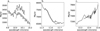 |
Fig. 1 Examples of intensity gaps observed in overlapping areas of adjacent cubes, obtained from MIRI-MRS data collected within the PDRs4All program (see Sect. 3.1 for more details). The spectra displayed correspond to the average spectra over the entire field of view for two overlapping sub-channels. Panel a: channel 2-medium and 2-long. Panel b: channel 2-long and 3-short. Panel c: channel 3-short and 3-medium. Fringes can be seen in Panel a, corresponding to a well-known phenomenon already documented by Argyriou et al. (2020). |
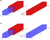 |
Fig. 2 Illustration of the stitching problem for two cubes. On the left, one can observe that the shortest wavelength cube in blue has a better spatial resolution (as illustrated by the finer grid) and a smaller field of view than the longest wavelength cube in red. The space-wavelength supports of the cubes partially overlap. The coarse stitching procedure shown in Fig. 1a sacrifices spatial resolution, while Haute Couture shown in Fig. 1b enables the reconstruction of a cube with the best spatial resolution over the full range of wavelengths. |
Name and wavelength range of the MIRI-MRS channels and sub-channels.
2 Haute Couture
2.1 Spectral stitching as a matrix completion problem
As introduced in Sect. 1, MIRI-MRS acquires spectra in four channels indexed by c (c = 1, . . . , 4). Each channel is divided into three sub-channels, referred to as short, medium, and long and shortened as s, m, and l, respectively. The spectral ranges of each sub-channel are reported in Table 1, as obtained from the STScI Jdocs1. Each sub-channel produces a space-wavelength cube as schematized in Fig. 2, where two of these cubes are depicted in blue and red. In the remainder of the paper, the spatial organization of the data is ignored, and we unfold each cube with respect to the spatial dimension (i.e., pixels). Thus the data associated with each cube can be represented as a matrix indexed by pixels and wavelengths. Formally, the matrix that gathers the data collected in sub-channel b ∈ {s, m, l} of channel c (c = 1, . . . , 4) is denoted as ![Mathematical equation: $\[\mathbf{X}^{c, b} \in \mathbb{R}_{+}^{\Lambda^{c, b} \times P^{c, b}}\]$](/articles/aa/full_html/2026/06/aa58120-25/aa58120-25-eq1.png) , where its rows index wavelengths while its columns index pixels. Specifically, the matrix Xc,b associated with the sub-channel (c,b) gathers spectra composed of Λc,b wavelengths and acquired over Pc,b spatial pixels.
, where its rows index wavelengths while its columns index pixels. Specifically, the matrix Xc,b associated with the sub-channel (c,b) gathers spectra composed of Λc,b wavelengths and acquired over Pc,b spatial pixels.
The resulting 12 sub-matrices can be arranged according to a suitable manner to form a larger matrix ![Mathematical equation: $\[\mathbf{X} \in \mathbb{R}_{+}^{\Lambda \times P}\]$](/articles/aa/full_html/2026/06/aa58120-25/aa58120-25-eq2.png) , as represented in Fig. 3, where
, as represented in Fig. 3, where ![Mathematical equation: $\[P=\sum_{c=1}^{4}\]$](/articles/aa/full_html/2026/06/aa58120-25/aa58120-25-eq3.png) ∑b∈{s,m,l} Pc,b and Λ is the total number of wavelengths over the spectral range covered by MIRI-MRS. It is worth noting that the spectral range of adjacent sub-matrices overlap for a few wavelengths, i.e.,
∑b∈{s,m,l} Pc,b and Λ is the total number of wavelengths over the spectral range covered by MIRI-MRS. It is worth noting that the spectral range of adjacent sub-matrices overlap for a few wavelengths, i.e., ![Mathematical equation: $\[\Lambda \neq {\sum}_{c=1}^{4}\]$](/articles/aa/full_html/2026/06/aa58120-25/aa58120-25-eq4.png) ∑b∈{s,m,l} Λc,b. This results in an almost block diagonal structure of the matrix X. In this figure, the white parts of the matrix correspond to unavailable (i.e., unobserved) data, specified by the symbol ∅. Because of these missing coefficients, the matrix X is said to be incomplete.
∑b∈{s,m,l} Λc,b. This results in an almost block diagonal structure of the matrix X. In this figure, the white parts of the matrix correspond to unavailable (i.e., unobserved) data, specified by the symbol ∅. Because of these missing coefficients, the matrix X is said to be incomplete.
The key rationale of the proposed stitching approach rests on the following insight: recovering all the missing coefficients of this matrix X would provide a comprehensive but redundant spatial-spectral description of the scene observed by MIRI-MRS. In particular, recovering the values of the sub-matrix S corresponding to the blue shaded area in Fig. 3 would produce a data cube at the spatial resolution of the channel 1-long (i.e., c = 1 and b = l) over the full spectral extent offered by MIRI-MRS, which is the main objective of this work. In other words, the spectral stitching task can be formulated as a matrix completion problem, i.e., recovery of the missing data in the matrix X. In this work, we target the channel 1-long to define the spatial resolutions of the stitched data because this leads to the best trade-off between high spatial resolution and a high signal-to-noise ratio. However, this arbitrary choice can be lifted since the proposed method will complete the full matrix X. In particular, we conducted some experiments while choosing the channel 1-short and 1-medium spatial resolutions. We obtained similar yet noisier structures than when targeting channel 1-long.
The following paragraphs detail the proposed two-step procedure to stitch the MIRI-MRS data while accommodating for intensity gaps between adjacent data cubes. This procedure consists of first rescaling the individual sub-matrices Xc,b homogeneously to correct the intensity gaps (see Sect. 2.2) and then filling the matrix X composed of the resulting intensity-corrected sub-matrices (see Sect. 2.3).
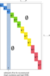 |
Fig. 3 Twelve unfolded cubes provided by the 12 sub-channels organized as sub-matrices of a larger matrix X with an almost block-diagonal structure. The wavelength range of the consecutive blocks overlaps for a few rows, corresponding to spectral bands observed by consecutive sub-channels. Blue blocks represent channel 1, green ones channel 2, yellow ones channel 3, and red ones channel 4. White and light blue parts correspond to unobserved coefficients. The light blue area corresponds to the area we are specifically interested in reconstructing. |
2.2 Intensity gaps correction
To mitigate the intensity gaps highlighted in Fig. 1, we introduced a novel preprocessing to homogenize the global intensities of the 12 cubes. This preprocessing consists of jointly adjusting a set of global scale parameters to maximize the fit between the parts of the cubes where spectral overlaps occur. With αc,b, we denote the scale parameter to be applied to the entries of the matrix Xc,b. As an example, referring to Fig. 3, the scale parameter, say α2,l, is computed by maximizing the fit between, on the one hand, the first rows of X2,l and the last rows of X2,m and, on the other hand, the last rows of X2,l and the first rows of X3,s. Because the matrices X2,m and X3,s themselves should be rescaled by the unknown scale parameters α2,m and α3,s, the optimal values of the whole set of scale parameters are interdependent, and they have to be adjusted jointly. Thankfully, when the fit is measured by the squared Euclidean distance between the portions of shared spectra, this optimization problem has a closed-form solution.
In practice at least one sub-channel must be chosen as an intensity reference to make the problem well-posed (otherwise, a trivial but inappropriate solution would be setting αc,b = 0 for all channels and sub-channels). In the experimental results conducted in Sect. 3, we fixed α1,s = α4,l = 1, and maximized the fit with respect to the ten remaining scale parameters. This amounts to trusting the calibration of the data observed in the lowest and highest ends of the wavelength range and updating the scales of the cubes in between. We note, however, that any other choice is possible. Technical details and the expressions of the resulting optimal scale parameters are reported in Appendix A.
2.3 Matrix completion
As explained in Sect. 2.1, recovering the missing coefficients in the full matrix X displayed in Fig. 3 can be interpreted as a matrix completion problem. Matrix completion aims at predicting missing values based on given observed values and the assumption of a latent matrix structure (see, e.g., Chi et al. 2019). In our case, and as in many other settings, it makes sense to assume that X has a “low-rank” structure, an assumption that has already underpinned several techniques of infrared spectroscopic data processing such as source separation (Rapacioli et al. 2005; Berné et al. 2007) or data fusion (Berné et al. 2010; Guilloteau et al. 2020a,b). It consists of imposing that the columns of X can be explained by linear combinations of elementary spectra embedded in noise. To further exploit the nonnegativity of the observed spectra, we propose performing this matrix completion by resorting to the technique of NMF (Lee & Seung 1999; Smaragdis et al. 2014). In other words, the missing entries are approximated by xij ≈ [WH]ij, where W and H are nonnegative matrices of size Λ × K and K × P estimated from the low-rank approximation of the observed entries. More precisely, we denote by 𝒪 the set of row and column indices of the observed values in X, i.e., the non-white part of X in Fig. 3 (or equivalently the supports of the sub-matrices Xc,b). The two matrices W and H are estimated by solving the following optimization problem:
![Mathematical equation: $\[\min _{\mathbf{W}, \mathbf{H} \geq 0} \sum_{(i, j) \in O} d\left(x_{i j} {\mid}[\mathbf{W} \mathbf{H}]_{i j}\right),\]$](/articles/aa/full_html/2026/06/aa58120-25/aa58120-25-eq5.png) (1)
(1)
where d(u|v) denotes a discrepancy measure between the nonnegative numbers u and v. In this study we leverage the work of Févotte & Idier (2011), who proposed easy-to-implement and efficient multiplicative updates for estimating W and H when d(·|·) is chosen as a so-called β-divergence. The β-divergence is a continuous family of measures of fit governed by a single shape parameter β ∈ ℝ that takes well-known divergences as special cases, namely the generalized Kullback-Leibler and Itakura-Saito divergences (β = 1, β = 0, respectively) and the square Euclidean distance (β = 2). Given a couple of matrices ![Mathematical equation: $\[\hat{\mathbf{W}}\]$](/articles/aa/full_html/2026/06/aa58120-25/aa58120-25-eq6.png) and
and ![Mathematical equation: $\[\hat{\mathbf{H}}\]$](/articles/aa/full_html/2026/06/aa58120-25/aa58120-25-eq7.png) that solve the minimization problem (1), the missing coefficients of X can be reconstructed as
that solve the minimization problem (1), the missing coefficients of X can be reconstructed as ![Mathematical equation: $\[\hat{x}_{i j}=[\hat{\mathbf{W}} \hat{\mathbf{H}}]_{i j}\]$](/articles/aa/full_html/2026/06/aa58120-25/aa58120-25-eq8.png) for (i, j) ∉ 𝒪.
for (i, j) ∉ 𝒪.
Like most NMF techniques, the algorithm tailored by Févotte & Idier (2011) is a descent algorithm that relies on alternating updates of W and H. Because of the bilinearity induced by the product WH, the objective function to minimize in Eq. (1) is nonconvex, and the algorithm is likely to produce local solutions that depend on the chosen starting point. As such, the initialization of the descent algorithm is an issue. We therefore investigate several initialization strategies in Sect. 3.2.
3 Application to MIRI-MRS data of the PDRs4All ERS program
3.1 Data and preprocessing
Data. The observations used in this work are part of the Early Release Science (ERS) program PDRs4All (Berné et al. 2022) and were obtained in January 2023. This program observed the Orion Bar with MIRI-MRS in a 1 × 9 pointing mosaic in the four channels. The mosaic is depicted in white in Fig. 4. Data were acquired with 47 groups per integration, one integration, and four dithers using the FASTR1 readout. The data were presented by Chown et al. (2024) and Van De Putte et al. (2024). The experiments reported in this paper used a single mosaic tile containing the protoplanetary disk d203-506 (highlighted in red in Fig. 4), which was also previously studied by Berné et al. (2023) and Zannese et al. (2024). Figure 5 presents the MIRI-MRS original data cubes with the initial field of view in each channel.
Data reduction pipeline. To illustrate the relevance of the proposed stitching method on a set of data representative of the current quality of JWST data products, the MIRI MRS data were reprocessed starting from the “uncal” files downloaded from MAST. For this purpose we used the scripts provided by the PDRs4All data reduction team and available from a public repository2 in combination with the JWST pipeline version 1.17.1 and CRDS context version “jwst_1322.pmap.” The standard pipeline stages were applied first with the default settings for stage 1 (detector1) and the following settings for stages 2 and 3. In stage 2, the image-to-image background subtraction method was applied (“bkg_subtract”) using the “rate” files obtained by applying stage 1 to the dedicated background observations for this program. The “residual_fringe” step was enabled, which reduced the residuals of fringes due to the reflections within the detector (Argyriou et al. 2020). In stage 3, we enabled the “outlier_detection” step and disabled the “cube_build” step so that the final products were the fully processed 2D IFU images (‘crf’ files). We then ran the “cube_build” step, which is based on the Drizzle algorithm (Law et al. 2023), and it led to a common spatial grid across all wavelengths for the data to be stitched. This choice was motivated by two main reasons: (i) Focusing on the exact intersection of fields of view with distinct spatial pixel resolutions would have led to a significant loss of information. (ii) Because of the lower spatial resolution, the data at longer wavelengths carry less information (in terms of numbers of pixels), which would have biased the results. This resampling could have been performed after data reduction during the preprocessing step (see below) by a naive spatial interpolation. Instead, this resampling was performed during the data reduction to benefit from the functionalities offered by the pipeline, which performs this interpolation more efficiently, using both spatial and spectral information.
Therefore, the “cube_build” step was performed with custom settings starting from the stage 3 “crf” files. The full specification of these settings was as follows. The position angle was set to “cube_pa=250.4,” which aligned with the orientation of the 9x1 mosaic. The pixel scale and field of view were set to those of channel 1 using “scale_xy=0.13,” “nspax_x=33,” and “nspax_y=39,” and the center coordinates were set to “ra_center=83.834782,” “dec_center=−5.418207.” For channel 1, the resulting cube had nearly identical properties to the one built with the default coordinate system. For the longer wavelength channels, the pixel scale of these custom cubes substantially oversampled the instrumental resolution; this was the expected type of input for the method presented in this work.
Preprocessing. The Haute Couture stitching method proposed in Sect. 2 assumes that the spectral grids between two adjacent cubes are the same for the shared wavelength range, which is not the case for the data provided by the reduction pipeline. As such, the data were spectrally resampled on a common wavelength grid with a consistent step using a linear 1D interpolation.
Additionally, the data contained saturated frames, spikes, and so-called bad pixels (i.e., outliers) that needed to be cleaned. Instead of merely discarding the saturated frames, they were replaced by corrected frames resulting from a spectral linear interpolation to avoid gaps with no data for some spectral bands. This step was shown to be of major importance. If the data cubes to be stitched contained one saturated frame, the stitched result might be significantly distorted. For instance, it may contain unexpected spatial patterns and significant spectral bias. Regarding the remaining spikes and bad pixels in each frame, they were automatically detected and corrected. A significant number of those anomalies exhibited structures with high intensity. To identify them, we implemented a robust anomaly detector following the strategy proposed by Anderson & Gordon (2011). In each frame ![Mathematical equation: $\[\mathbf{X}_{i,:}^{c, b}\]$](/articles/aa/full_html/2026/06/aa58120-25/aa58120-25-eq9.png) associated with a given channel c and sub-channel b the median pixel value
associated with a given channel c and sub-channel b the median pixel value ![Mathematical equation: $\[\bar{x}_{i}^{c, b}=\operatorname{median}(\mathbf{X}_{i,:}^{c, b})\]$](/articles/aa/full_html/2026/06/aa58120-25/aa58120-25-eq10.png) was first computed as a robust counterpart of the mean pixel values. Each pixel value significantly far from this robust mean was then identified as an anomaly. More precisely, a pixel value
was first computed as a robust counterpart of the mean pixel values. Each pixel value significantly far from this robust mean was then identified as an anomaly. More precisely, a pixel value ![Mathematical equation: $\[x_{i j}^{c, b}\]$](/articles/aa/full_html/2026/06/aa58120-25/aa58120-25-eq11.png) such that
such that ![Mathematical equation: $\[|x_{i j}^{c, b}-\bar{x}_{i}^{c, b}|>t \times \operatorname{MAD}(\mathbf{X}_{i,:}^{c, b})\]$](/articles/aa/full_html/2026/06/aa58120-25/aa58120-25-eq12.png) was flagged as an anomaly, where
was flagged as an anomaly, where ![Mathematical equation: $\[\operatorname{MAD}(\mathbf{X}_{i,:}^{c, b})=\operatorname{median}(x_{i, j}^{c, b}-\bar{x}_{i}^{c, b})\]$](/articles/aa/full_html/2026/06/aa58120-25/aa58120-25-eq13.png) computes the median absolute deviation and t is a cutoff parameter that needs to be adjusted for each channel and sub-channel. The pixel values detected as anomalies were finally replaced by the average of their four spatially nearest neighbors.
computes the median absolute deviation and t is a cutoff parameter that needs to be adjusted for each channel and sub-channel. The pixel values detected as anomalies were finally replaced by the average of their four spatially nearest neighbors.
Finally, we created a mask containing only the most informative pixels. A pixel value was flagged as not carrying any information if its value was NaN. For each cube, the mask corresponds to the spatial pixels that have more than 99% spectral information (i.e., that are not NaN). In the mask, the star at the top of our field of view was removed because it is saturated in most of the wavelength range and the spectra are not exploitable.
 |
Fig. 4 Colorized NIRCam image of the Orion Bar of the PDRs4All ERS program (Berné et al. 2024). Filters F140M and F210M are in blue; F277W, F300M, F323N, and F335M are in green; F405N is in orange; and F444W, F480M, and F470N are in red. The pattern in white is the MIRI-MRS mosaic footprint. The red box corresponds to the pointing used in this article. |
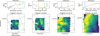 |
Fig. 5 First row: average spectra over the entire field of view of each channel (shown in the second row). A different color (blue, orange, green) is used for each sub-channel (short, medium, long). Second row: MIRI-MRS images at different wavelengths (the images are aligned). It can be observed that the field of view increases with the channel but the spatial resolution deteriorates. |
3.2 Choice of the parameters and initialization
As discussed in Sect. 2, Haute Couture requires a few hyperparameters to be set by the end user. A first hyperparameter is the value of β, i.e., the shape parameter of the divergence used as a measure of the fit in NMF. As thoroughly discussed by Févotte & Idier (2011), the β-divergence is a log-likelihood in disguise, and choosing β is similar to making a noise assumption. The range of practical values is generally β ∈ [0, 2], with β = 0 corresponding to multiplicative Gamma noise and β = 2 corresponding to additive Gaussian noise. Choosing β = 1 (generalized Kullback-Leibler divergence), corresponding to a Poisson-like continuous distribution, has been shown to offer an excellent trade-off in many applications. In particular, it was advocated for in the work by Berné et al. (2007) for source separation of similar mid-IR data using NMF.
A second hyperparameter to set is K, i.e., the rank of the factorization (the common dimension of W and H). A suitable value needs to capture the latent structure in the data while preventing overfitting (i.e., modeling the noise rather than the inherent phenomena that explain the data). We followed a trial and error approach by assessing the quality of the reconstruction with a set of candidate values for K, namely K ∈ [2, 4, 6, 10, 15]. We considered only channel 2 and 3 in order to save computing time. For every couple of estimated matrices W and H, we then calculated the correlation between the reconstruction and the MIRI-MRS spectra (spectra after preprocessing in order to compare) for each sub-channel and the average of the sub-channel. For all K, the average correlation was 0.935 ± 0.0006. The algorithm was not very sensitive to the value of K in our example, and thus, we chose K = 6 since it maximized the correlation.
In addition to choosing the hyperparameters β and K, Haute Couture requires choosing an initialization strategy for W and H in the NMF algorithm. We empirically assessed the performance of three methods: (i) random initialization, (ii) using the outputs of the K-means clustering algorithm, and (iii) using the maximum angle source separation (MASS) technique proposed by Boulais et al. (2021). As for the adjusting of the hyperparameters β and K, we conducted an exhaustive set of experiments to assess the performance of each of these three methods in reaching the best fit, with β = 1, K = 6, again using channel 2 and 3 to save computing time. Our experiments revealed that K-means and MASS return similar results and a much better performance than random initialization. We favored MASS in the experiments, however, as it was initially designed for infrared astronomical hyperspectral cubes.
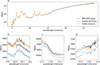 |
Fig. 6 Top: average spectrum of the MIRI-MRS data after removing the saturated frames, spikes, and bad pixels (black curve); average of the stitched data recovered by Haute Couture (orange curve); and average of the result of the coarse stitching procedure (blue curve). Bottom: zoom-ins on the spectral ranges where overlap occurs between contiguous sub-channels (as already depicted in Fig. 1). |
4 Results
4.1 Stitching results
Figure 6 (top) displays the average spectrum of the MIRI-MRS data over the entire field of view after removing the saturated frames, the spikes, and the bad pixels, as explained in Sect. 3.1. It depicts the average spectrum of the stitched data ![Mathematical equation: $\[\hat{\mathbf{S}}\]$](/articles/aa/full_html/2026/06/aa58120-25/aa58120-25-eq14.png) recovered by Haute Couture (corresponding to the values in channel 1-long of the sub-matrix highlighted in the blue shaded area of Fig. 3). This result is compared to the product given by the coarse stitching procedure explained in Appendix B. The figure also displays three zoom-ins of the spectral ranges where overlap occur between contiguous sub-channels (bottom). By design, the Haute Couture stitched data average spectrum is continuous, i.e., the spectral gaps exhibited in the original MIRI-MRS data have been removed. It is also worth noting that the fit between the original and Haute Couture reconstructed data is rather tight over the full spectral range.
recovered by Haute Couture (corresponding to the values in channel 1-long of the sub-matrix highlighted in the blue shaded area of Fig. 3). This result is compared to the product given by the coarse stitching procedure explained in Appendix B. The figure also displays three zoom-ins of the spectral ranges where overlap occur between contiguous sub-channels (bottom). By design, the Haute Couture stitched data average spectrum is continuous, i.e., the spectral gaps exhibited in the original MIRI-MRS data have been removed. It is also worth noting that the fit between the original and Haute Couture reconstructed data is rather tight over the full spectral range.
Figure 7 displays the preprocessed MIRI-MRS data before stitching and compares the final products resulting from the coarse stitching procedure and from the proposed Haute Couture method. This figure also depicts the Haute Couture product after undergoing a convolution with a Gaussian filter whose standard deviation ![Mathematical equation: $\[\sigma=\frac{1.22 \lambda}{2 \sqrt{2 ~\ln~ 2} D}\]$](/articles/aa/full_html/2026/06/aa58120-25/aa58120-25-eq15.png) has been specifically designed to mimic the effect of the MIRI PSF, where λ is the considered wavelength and D is the mirror diameter. The resulting convolved product can then also be fairly compared to the original MIRI-MRS data as a validation step.
has been specifically designed to mimic the effect of the MIRI PSF, where λ is the considered wavelength and D is the mirror diameter. The resulting convolved product can then also be fairly compared to the original MIRI-MRS data as a validation step.
In the first row, corresponding to data and results at 5.61 μm (channel 1), the Haute Couture image appears as significantly denoised and exhibits the same spatial resolution as the original data. This was expected since, as motivated in Sect. 2.1, the Haute Couture stitching procedure targets the spatial resolutions of channel 1-long (blue shaded area in Fig. 3). Moreover, the observed denoising effect can be attributed to the low-rank factor model underlying Haute Couture. By implicitly representing the spectral data into a K-dimensional subspace, the proposed stitching approach preserves the essential physical information while effectively filtering out most of the noise. The second row, associated with results at 9.29 μm (channel 2), shows a lightly denoised and more contrasted Haute Couture image compared to the MIRI-MRS image. At 12.27 μm (channel 3), the Haute Couture image is sharper and more contrasted than the MIRI-MRS data. Interestingly, the spatial structure of the d203-506 protoplanetary disk, which is known to be present in the considered astrophysical scene Berné et al. (2024), is well reconstructed. The MIRI-MRS image at 20.42 μm (channel 4) does not contain any particular spatial structure and the d203-506 protoplanetary disk is no longer visible. In the Haute Couture image, the spatial structures are well recovered.
Conversely, in all channels, the product resulting from the coarse stitching procedure is affected by a worse contrast and a clear underestimation of the spectral flux density already highlighted in Fig. 6. It is also worth noting that the loss in spatial resolution is significant. This was expected since the coarse stitching procedure targets the poorest resolution offered by the data cubes to be stitched.
The most straightforward way to validate an algorithm is to test it against ground truth data, as is often possible with Earth observation data. However, in the case of astronomical data, obtaining ground truth is impossible. A widely used alternative consists of validating the algorithm using simulated data. This strategy has been followed for instance by Guilloteau et al. (2020b) to validate data fusion algorithms by generating simulated NIRCam and NIRSpec data. Simulating MIRI-MRS data, however, is more challenging (Hadj-Youcef et al. 2017). The Pandeia tool (Pontoppidan et al. 2016) can produce simulated MIRI-MRS data, but it only allows simulation of simple scenes. The MRISim tool (Klaassen et al. 2021) allows for more complex scenes. However, to our knowledge, the public version of this software has not been updated since the launch of JWST, and therefore the tool may not provide data that are directly comparable to real observations. In this context, as a sanity check, we compare in Fig. 7 the results of degraded Haute Couture data after undergoing the Gaussian smoothing (Col. 4) and those of the original MIRI-MRS data (Col. 1). It can be seen that there is a good qualitative agreement in terms of the spatial textures between images of Cols. 1 and 4, especially in channels 1 and 2. At longer wavelengths, the images differ notably in the right part of the scene. This can be explained by the masking procedure implemented during the preprocessing, which removes pixels associated with the star located in this area (see Sect. 3.1).
4.2 Error propagation
The MIRI-MRS cubes provided by the pipeline as detailed in Sect. 3.1 and stitched in Sect. 4.1 are provided with so-called error cubes (specified by the extension ERR). More precisely, each data cube Xc,b composing the matrix X depicted in Fig. 3 is granted with an error matrix denoted ΔXc,b. To quantify the relative amount of error contained in the original MIRI-MRS data to be stitched, we first evaluated the signal-to-error ratio (SER) defined as
![Mathematical equation: $\[\mathrm{SER}=10 ~\log \frac{\sum_{c, b}\left\|\mathbf{X}^{c, b}\right\|_2^2}{\sum_{c, b}\left\|\Delta \mathbf{X}^{c, b}\right\|_2^2}=53.09 \mathrm{dB}.\]$](/articles/aa/full_html/2026/06/aa58120-25/aa58120-25-eq16.png) (2)
(2)
We then assessed the propagation of this error when performing stitching. To do so, we introduced the set of data matrices ![Mathematical equation: $\[\mathbf{X}_{+}^{c, b}=\mathbf{X}^{c, b}+\Delta \mathbf{X}^{c, b}\]$](/articles/aa/full_html/2026/06/aa58120-25/aa58120-25-eq17.png) and
and ![Mathematical equation: $\[\mathbf{X}_{-}^{c, b}=\mathbf{X}^{c, b}-\Delta \mathbf{X}^{c, b}\]$](/articles/aa/full_html/2026/06/aa58120-25/aa58120-25-eq18.png) corresponding to the original data positively and negatively perturbed by the error term in each channel c and sub-channel b. These sub-matrices were rearranged to form the incomplete matrices X+ and X− as perturbed counterparts of the original incomplete matrix X introduced in Sect. 2 (see also Fig. 3). The completion procedure detailed in Sect. 2.3 was applied on these two incomplete matrices X+ and X−, yielding the pair of stitched data
corresponding to the original data positively and negatively perturbed by the error term in each channel c and sub-channel b. These sub-matrices were rearranged to form the incomplete matrices X+ and X− as perturbed counterparts of the original incomplete matrix X introduced in Sect. 2 (see also Fig. 3). The completion procedure detailed in Sect. 2.3 was applied on these two incomplete matrices X+ and X−, yielding the pair of stitched data ![Mathematical equation: $\[\hat{\mathbf{S}}_{+}\]$](/articles/aa/full_html/2026/06/aa58120-25/aa58120-25-eq19.png) and
and ![Mathematical equation: $\[\mathbf{\hat { S }}_{-}\]$](/articles/aa/full_html/2026/06/aa58120-25/aa58120-25-eq20.png) recovered by the proposed method Haute Couture. Finally, the propagation of the error was evaluated by quantifying how much the original amount of error translates into the perturbed data after undergoing stitching. Formally, we computed the SER associated with the positively and negatively perturbed data as
recovered by the proposed method Haute Couture. Finally, the propagation of the error was evaluated by quantifying how much the original amount of error translates into the perturbed data after undergoing stitching. Formally, we computed the SER associated with the positively and negatively perturbed data as
![Mathematical equation: $\[\mathrm{SER}_{+}=10 ~\log \frac{\|\hat{\mathbf{S}}\|_2^2}{\left\|\Delta \hat{\mathbf{S}}_{+}\right\|_2^2} \quad \text { and } \quad \mathrm{SER}_{-}=10 ~\log \frac{\|\hat{\mathbf{S}}\|_2^2}{\left\|\Delta \hat{\mathbf{S}}_{-}\right\|_2^2},\]$](/articles/aa/full_html/2026/06/aa58120-25/aa58120-25-eq21.png) (3)
(3)
where ![Mathematical equation: $\[\Delta \hat{\mathbf{S}}_{ \pm}=\hat{\mathbf{S}}_{ \pm}-\hat{\mathbf{S}}\]$](/articles/aa/full_html/2026/06/aa58120-25/aa58120-25-eq27.png) measures the discrepancy between the stitched spectra
measures the discrepancy between the stitched spectra ![Mathematical equation: $\[\hat{\mathbf{S}}\]$](/articles/aa/full_html/2026/06/aa58120-25/aa58120-25-eq28.png) resulting from the original data and the stitched spectra
resulting from the original data and the stitched spectra ![Mathematical equation: $\[\hat{\mathbf{S}}_{ \pm}\]$](/articles/aa/full_html/2026/06/aa58120-25/aa58120-25-eq29.png) resulting from the perturbed data.
resulting from the perturbed data. ![Mathematical equation: $\[\Delta \hat{\mathbf{S}}_{ \pm}\]$](/articles/aa/full_html/2026/06/aa58120-25/aa58120-25-eq30.png) is considered as the propagated error. We obtained SER+ = 33.43 dB and SER_ = 34.25 dB. The overall procedure is sketched out in Fig. 8. It appears that the SER deteriorates by about 20 dB, which may be explained by the fact that the error terms ΔXc,b do not likely follow the NMF model underlying the completion procedure detailed in Sect. 2.3. Yet, more importantly, the amount of additional error induced by Haute Couture remains of low magnitude with respect to both the original error and the energy of the stitched data.
is considered as the propagated error. We obtained SER+ = 33.43 dB and SER_ = 34.25 dB. The overall procedure is sketched out in Fig. 8. It appears that the SER deteriorates by about 20 dB, which may be explained by the fact that the error terms ΔXc,b do not likely follow the NMF model underlying the completion procedure detailed in Sect. 2.3. Yet, more importantly, the amount of additional error induced by Haute Couture remains of low magnitude with respect to both the original error and the energy of the stitched data.
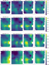 |
Fig. 7 Comparison between the MIRI-MRS data obtained using the JWST pipeline cube_build (Col. 1), the result of the coarse stitching procedure (Col. 2), the stitched data produced by Haute Couture (Col. 3), and this final product convolved with a Gaussian filter (Col. 4) in each channel at a given wavelength. The same color bar (in MJy/sr) is used in each row, and the data in Cols. 1, 3, and 4 share the same mask. The red circles correspond to the emplacement of the d203-506 protoplanetary disk. The loss of spatial resolution is also clearly visible when performing a coarse stitching. |
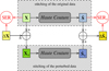 |
Fig. 8 Quantification of the error propagation. The amount of error, SER, before stitching was evaluated from the original data contained in X (light green box) and the error matrix ΔX (light yellow box). The original data X were processed by Haute Couture to produce the stitched spectra |
![Mathematical equation: $\[\hat{\mathbf{S}}\]$](/articles/aa/full_html/2026/06/aa58120-25/aa58120-25-eq22.png)
![Mathematical equation: $\[\hat{\mathbf{S}}_{ \pm}\]$](/articles/aa/full_html/2026/06/aa58120-25/aa58120-25-eq23.png)
![Mathematical equation: $\[\Delta \hat{\mathbf{S}}_{ \pm}\]$](/articles/aa/full_html/2026/06/aa58120-25/aa58120-25-eq24.png)
![Mathematical equation: $\[\hat{\mathbf{S}}\]$](/articles/aa/full_html/2026/06/aa58120-25/aa58120-25-eq25.png)
![Mathematical equation: $\[\Delta \hat{\mathbf{S}}_{ \pm}\]$](/articles/aa/full_html/2026/06/aa58120-25/aa58120-25-eq26.png)
5 Conclusion
In this paper, we have presented a new stitching algorithm named Haute Couture that provides near-optimal assembly of MIRI-MRS spectral cubes. Haute Couture allows spatial information to be preserved throughout the overall spectral range covered by JWST. By applying the algorithm to real observations, we showed that Haute Couture is able to recover spatial structures that are not preserved by a coarse stitching procedure. Our proposed approach relies on the formulation of the stitching task as a matrix completion problem, which is subsequently solved by NMF. In principle, the versatility of this formulation makes the proposed approach applicable to spectral cubes provided by other spatial instruments, such as NIRSpec (also on board JWST) or by ground-based IFUs.
Data availability
The source code for this method is available through https://github.com/acanin/hautecouture. The Haute Couture cube presented in this paper is available at the CDS via https://cdsarc.cds.unistra.fr/viz-bin/cat/J/A+A/710/A6.
Acknowledgements
This work is partially supported by the Artificial and Natural Intelligence Toulouse Institute (ANITI), funded by the France 2030 program under the grant agreement ANR-23-IACL-0002. This work is funded by the Centre National d’Etudes Spatiales (CNES) through the APR program.
References
- Anderson, R. E., & Gordon, K. D. 2011, PASP, 123, 1237 [NASA ADS] [CrossRef] [Google Scholar]
- Argyriou, I., Wells, M., Glasse, A., et al. 2020, A&A, 641, A150 [NASA ADS] [CrossRef] [EDP Sciences] [Google Scholar]
- Argyriou, I., Glasse, A., Law, D. R., et al. 2023, A&A, 675, A111 [NASA ADS] [CrossRef] [EDP Sciences] [Google Scholar]
- Berné, O., Joblin, C., Deville, Y., et al. 2007, A&A, 469, 575 [NASA ADS] [CrossRef] [EDP Sciences] [Google Scholar]
- Berné, O., Helens, A., Pilleri, P., & Joblin, C. 2010, in 2010 2nd Workshop on Hyperspectral Image and Signal Processing: Evolution in Remote Sensing, IEEE, 1 [Google Scholar]
- Berné, O., Habart, É., Peeters, E., et al. 2022, PASP, 134, 054301 [CrossRef] [Google Scholar]
- Berné, O., Martin-Drumel, M.-A., Schroetter, I., et al. 2023, Nature, 621, 56 [CrossRef] [Google Scholar]
- Berné, O., Habart, E., Peeters, E., et al. 2024, Science, 383, 988 [Google Scholar]
- Boulais, A., Berné, O., Faury, G., & Deville, Y. 2021, A&A, 647, A105 [EDP Sciences] [Google Scholar]
- Chi, Y., Lu, Y. M., & Chen, Y. 2019, IEEE Trans. Signal Process., 67, 5239 [Google Scholar]
- Chown, R., Sidhu, A., Peeters, E., et al. 2024, A&A, 685, A75 [NASA ADS] [CrossRef] [EDP Sciences] [Google Scholar]
- Févotte, C., & Idier, J. 2011, Neural Computat., 23, 2421 [Google Scholar]
- Gardner, J. P., Mather, J. C., Clampin, M., et al. 2006, Space Sci. Rev., 123, 485 [Google Scholar]
- Guilloteau, C., Oberlin, T., Berne, O., & Dobigeon, N. 2020a, IEEE Trans. Computat. Imaging, 6, 1362 [Google Scholar]
- Guilloteau, C., Oberlin, T., Berné, O., Habart, É., & Dobigeon, N. 2020b, AJ, 160, 28 [NASA ADS] [CrossRef] [Google Scholar]
- Hadj-Youcef, M. A., Orieux, F., Fraysse, A., & Abergel, A. 2017, in 2017 25th European Signal Processing Conference (EUSIPCO), IEEE, 503 [Google Scholar]
- Houck, J. R., Roellig, T. L., van Cleve, J., et al. 2004, ApJS, 154, 18 [NASA ADS] [CrossRef] [Google Scholar]
- Klaassen, P. D., Geers, V. C., Beard, S. M., et al. 2021, MNRAS, 500, 2813 [Google Scholar]
- Law, D. R. E., Morrison, J., Argyriou, I., et al. 2023, AJ, 166, 45 [NASA ADS] [CrossRef] [Google Scholar]
- Lee, D. D., & Seung, H. S. 1999, Nature, 401, 788 [Google Scholar]
- Perrin, M. D., Sivaramakrishnan, A., Lajoie, C.-P., et al. 2014, SPIE Conf. Ser., 9143, 91433X [NASA ADS] [Google Scholar]
- Pontoppidan, K. M., Pickering, T. E., Laidler, V. G., et al. 2016, SPIE Conf. Ser., 9910, 991016 [NASA ADS] [Google Scholar]
- Rapacioli, M., Joblin, C., Boissel, P., Calvo, F., & Spiegelman, F. 2005, in ESA Special Publication, 577, ed. A. Wilson, 409 [Google Scholar]
- Rieke, G. H., Wright, G. S., Böker, T., et al. 2015, The mid-infrared instrument for the James Webb Space Telescope, I: Introduction, Tech. Rep. Technical Report JWST-STScI-000001, STScI [Google Scholar]
- Sandstrom, K. M., Bolatto, A. D., Draine, B. T., Bot, C., & Stanimirović, S. 2010, ApJ, 715, 701 [NASA ADS] [CrossRef] [Google Scholar]
- Smaragdis, P., Févotte, C., Mysore, G. J., Mohammadiha, N., & Hoffman, M. 2014, IEEE Signal Process. Mag., 31, 66 [Google Scholar]
- Van De Putte, D., Meshaka, R., Trahin, B., et al. 2024, A&A, 687, A86 [NASA ADS] [CrossRef] [EDP Sciences] [Google Scholar]
- Wells, M., Pel, J.-W., Glasse, A., et al. 2015, PASP, 127, 646 [NASA ADS] [CrossRef] [Google Scholar]
- Werner, M. W., Roellig, T. L., Low, F. J., et al. 2004, ApJS, 154, 1 [NASA ADS] [CrossRef] [Google Scholar]
- Wright, G. S., Rieke, G. H., Glasse, A., et al. 2023, PASP, 135, 048003 [NASA ADS] [CrossRef] [Google Scholar]
- Zannese, M., Tabone, B., Habart, E., et al. 2024, Nat. Astron., 8, 577 [Google Scholar]
Appendix A Joint scale parameter estimation
This appendix details the approach introduced in Sect. 2.2 and implemented to mitigate intensity gaps observed between the sub-channels of MIRI-MRS data cubes (see Fig. 1). To ease the presentation of the method, we introduce the one-to-one mapping between the couple (c,b) ∈ {1, . . . , 4} × {s, m, l} which indexes a given sub-channel b of a given channel c and the integer i ∈ {1, . . . , 12} which indexes the sub-matrix composing X according to the particular order represented in Fig. 3. Thus in what follows, the sub-matrix Xc,b is simply denoted as Xi, leading to the alternate representation of the matrix X depicted in Fig. A.1.
The intensity gap correction aims at estimating a set of 12 scale parameters α = [α1, . . . , α12]T to be applied to the 12 data matrices {X1, . . . , X12}, respectively. By the very specific nature of the data acquisition, the wavelength range associated with the top rows (resp. bottom) of the matrix Xi emphasized as green (resp. blue) boxes in Fig. A.1 overlaps with the bottom rows of the matrix Xi–1 (resp. top of Xi+1) emphasized as blue (resp. green) boxes in Fig. A.1. It is worth noting that contiguous green and blue boxes frame portions of spectra that correspond to the same spatial locations at the same wavelengths. Thus the proposed approach consists in jointly adjusting the scale parameters by ensuring that the portions of pixel spectra located in the blue boxes match as much as possible the portions of the pixel spectra in the contiguous green boxes. Formally, the spatial average of the top (resp. bottom) rows of Xi where such overlap occurs is denoted by ![Mathematical equation: $\[\overline{\boldsymbol{\mu}}^{i}\]$](/articles/aa/full_html/2026/06/aa58120-25/aa58120-25-eq31.png) (resp.
(resp. ![Mathematical equation: $\[\underline{\boldsymbol{\mu}}^{i}\]$](/articles/aa/full_html/2026/06/aa58120-25/aa58120-25-eq32.png) ), see Fig. A.1. Maximizing the fit between
), see Fig. A.1. Maximizing the fit between ![Mathematical equation: $\[\alpha^{i} \underline{\boldsymbol{\mu}}^{i}\]$](/articles/aa/full_html/2026/06/aa58120-25/aa58120-25-eq33.png) and
and ![Mathematical equation: $\[\alpha^{i+1} \overline{\boldsymbol{\mu}}^{i-1}\]$](/articles/aa/full_html/2026/06/aa58120-25/aa58120-25-eq34.png) , for i = 1, . . . , 11, boils down to solving the optimization problem
, for i = 1, . . . , 11, boils down to solving the optimization problem
![Mathematical equation: $\[\min _{\boldsymbol{\alpha}} \sum_{i=1}^{11}\left\|\alpha^i \underline{\boldsymbol{\mu}}^i-\alpha^{i+1} \overline{\boldsymbol{\mu}}^{i+1}\right\|_2^2,\]$](/articles/aa/full_html/2026/06/aa58120-25/aa58120-25-eq35.png) (A.1)
(A.1)
with α = [α1, . . . , α12]T. The problem as formulated by Eq. (A.1) is ill-posed since one optimal solution is α* = [0, . . . , 0]T, i.e., setting all the sub-matrices to zero. To remove this trivial, inappropriate solution, one or more sub-channel serve as intensity references, with scale parameters fixed to an arbitrary value. In particular, in this work we assume that channels 1 and 12 have been properly calibrated and set α1 = α12 = 1, but the proposed methodology may apply with any other arbitrary choices. Thus, we introduced the sub-vector of scale parameters ![Mathematical equation: $\[\tilde{\boldsymbol{\alpha}}=\left[\alpha^{2}, \ldots, \alpha^{11}\right]^{T}\]$](/articles/aa/full_html/2026/06/aa58120-25/aa58120-25-eq36.png) and reformulated the problem (A.1) as
and reformulated the problem (A.1) as
![Mathematical equation: $\[\min _{\tilde{\boldsymbol{\alpha}}} \mathcal{J}(\tilde{\boldsymbol{\alpha}}) \quad \text { with } \quad \mathcal{J}(\tilde{\boldsymbol{\alpha}})=\sum_{i=2}^{10}\left\|\alpha^i \underline{\boldsymbol{\mu}}^i-\alpha^{i+1} \overline{\boldsymbol{\mu}}^{i+1}\right\|_2^2 \text {. }\]$](/articles/aa/full_html/2026/06/aa58120-25/aa58120-25-eq37.png) (A.2)
(A.2)
The criterion ![Mathematical equation: $\[C(\tilde{\boldsymbol{\alpha}})\]$](/articles/aa/full_html/2026/06/aa58120-25/aa58120-25-eq38.png) to be minimized is smooth and convex. Problem (A.2) has a unique solution that obeys
to be minimized is smooth and convex. Problem (A.2) has a unique solution that obeys
![Mathematical equation: $\[\nabla_{\tilde{\alpha}} \mathcal{J}(\tilde{\alpha})=0,\]$](/articles/aa/full_html/2026/06/aa58120-25/aa58120-25-eq39.png) (A.3)
(A.3)
where ∇ denotes the gradient operator. Trivial algebra shows that Eq. (A.3) is equivalent to solving the linear problem
![Mathematical equation: $\[\mathbf{M} \tilde{\alpha}=\mathbf{b},\]$](/articles/aa/full_html/2026/06/aa58120-25/aa58120-25-eq40.png) (A.4)
(A.4)
where M and b are the square matrix and vector of sizes ten given by
![Mathematical equation: $\[\mathbf{M}=\left(\begin{array}{ccccc}1 & -\frac{\left\langle\underline{\boldsymbol{\mu}}^2, \overline{\boldsymbol{\mu}}^3\right\rangle}{\left\|\underline{\boldsymbol{\mu}}^2\right\|_2^2+\left\|\overline{\boldsymbol{\mu}}^2\right\|_2^2} & 0 & \ldots & 0 \\-\frac{\left\langle\underline{\boldsymbol{\mu}}^2, \overline{\boldsymbol{\mu}}^3\right\rangle}{\left\|\underline{\boldsymbol{\mu}}^3\right\|_2^2+\left\|\overline{\boldsymbol{\mu}}^3\right\|_2^2} & 1 & -\frac{\left\langle\underline{\boldsymbol{\mu}}^3, \overline{\boldsymbol{\mu}}^4\right\rangle}{\left\|\underline{\boldsymbol{\mu}}^3\right\|_2^2+\left\|\overline{\boldsymbol{\mu}}^3\right\|_2^2} & \ddots & \vdots \\0 & -\frac{\left\langle\underline{\boldsymbol{\mu}}^3, \overline{\boldsymbol{\mu}}^4\right\rangle}{\left\|\underline{\boldsymbol{\mu}}^4\right\|_2^2+\left\|\overline{\boldsymbol{\mu}}^4\right\|_2^2} & 1 & \ddots & 0 \\\vdots & \ddots & \ddots & \ddots & -\frac{\left\langle\underline{\boldsymbol{\mu}}^{10}, \overline{\boldsymbol{\mu}}^{11}\right\rangle}{\left\|\underline{\boldsymbol{\mu}}^{10}\right\|_2^2+\left\|\overline{\boldsymbol{\mu}}^{10}\right\|_2^2} \\0 & \cdots & 0 & -\frac{\left\langle\underline{\boldsymbol{\mu}}^{10}, \overline{\boldsymbol{\mu}}^{11}\right\rangle}{\left\|\underline{\boldsymbol{\mu}}^{11}\right\|_2^2+\left\|\overline{\boldsymbol{\mu}}^{11}\right\|_2^2} & 1\end{array}\right) \text { and } \quad \mathbf{b}=\left(\begin{array}{c}\frac{\left\langle\underline{\boldsymbol{\mu}}^1, \overline{\boldsymbol{\mu}}^2\right\rangle}{\left\|\underline{\boldsymbol{\mu}}^2\right\|_2^2+\mid \overline{\boldsymbol{\mu}}^2 \|_2^2} \\0 \\\vdots \\0 \\\frac{\left\langle\underline{\boldsymbol{\mu}}^{11}, \overline{\boldsymbol{\mu}}^{12}\right\rangle}{\left\|\underline{\boldsymbol{\mu}}^{11}\right\|_2^2+\left\|\overline{\boldsymbol{\mu}}^{11}\right\|_2^2}\end{array}\right).\]$](/articles/aa/full_html/2026/06/aa58120-25/aa58120-25-eq41.png)
The optimal scale parameters are thus given by ![Mathematical equation: $\[\tilde{\boldsymbol{\alpha}}^{*}=\mathbf{M}^{-1} \mathbf{b}\]$](/articles/aa/full_html/2026/06/aa58120-25/aa58120-25-eq42.png) .
.
Appendix B Coarse stitching
In this section we present how we produce the coarse stitching presented as comparison in Sect. 4. We use the MIRI-MRS original data cubes presented in Sect. 3.1 and Fig. 5.
Field of view. The first step is to have a common field of view corresponding to the intersection of each field of view. A exact common spatial grid is impossible due to the pixel size of each channel.
Convolution with PSF. Each channel and sub-channel is convolved with the PSF of the channel 4-long using the library stpsf (Perrin et al. 2014). We use the Fourier transform to perform the convolution. Then we calibrate the flux in order to have the same flux than before because there is a side effect when convoluting the data that loses flux. This effect is particularly visible at large wavelength because these are fewer pixels.
Reprojection. To compare the same pixels, we need a common spatial grid for every channel and sub-channel. Hence, those are reprojected in the spatial grid of the channel 4-long using the function griddata of the library SciPy.
Stitching. The stitching is performed individually for each spatial pixel. The channel 1-short is used as reference for the calibration. For each pixel the average of the fluxes are calculated on the spectral overlap between two successive sub-channel. Then the spectrum that is not the reference is scaled using the ratio of the average.
All Tables
All Figures
|
Fig. 1 Examples of intensity gaps observed in overlapping areas of adjacent cubes, obtained from MIRI-MRS data collected within the PDRs4All program (see Sect. 3.1 for more details). The spectra displayed correspond to the average spectra over the entire field of view for two overlapping sub-channels. Panel a: channel 2-medium and 2-long. Panel b: channel 2-long and 3-short. Panel c: channel 3-short and 3-medium. Fringes can be seen in Panel a, corresponding to a well-known phenomenon already documented by Argyriou et al. (2020). |
| In the text | |
|
Fig. 2 Illustration of the stitching problem for two cubes. On the left, one can observe that the shortest wavelength cube in blue has a better spatial resolution (as illustrated by the finer grid) and a smaller field of view than the longest wavelength cube in red. The space-wavelength supports of the cubes partially overlap. The coarse stitching procedure shown in Fig. 1a sacrifices spatial resolution, while Haute Couture shown in Fig. 1b enables the reconstruction of a cube with the best spatial resolution over the full range of wavelengths. |
| In the text | |
|
Fig. 3 Twelve unfolded cubes provided by the 12 sub-channels organized as sub-matrices of a larger matrix X with an almost block-diagonal structure. The wavelength range of the consecutive blocks overlaps for a few rows, corresponding to spectral bands observed by consecutive sub-channels. Blue blocks represent channel 1, green ones channel 2, yellow ones channel 3, and red ones channel 4. White and light blue parts correspond to unobserved coefficients. The light blue area corresponds to the area we are specifically interested in reconstructing. |
| In the text | |
|
Fig. 4 Colorized NIRCam image of the Orion Bar of the PDRs4All ERS program (Berné et al. 2024). Filters F140M and F210M are in blue; F277W, F300M, F323N, and F335M are in green; F405N is in orange; and F444W, F480M, and F470N are in red. The pattern in white is the MIRI-MRS mosaic footprint. The red box corresponds to the pointing used in this article. |
| In the text | |
|
Fig. 5 First row: average spectra over the entire field of view of each channel (shown in the second row). A different color (blue, orange, green) is used for each sub-channel (short, medium, long). Second row: MIRI-MRS images at different wavelengths (the images are aligned). It can be observed that the field of view increases with the channel but the spatial resolution deteriorates. |
| In the text | |
|
Fig. 6 Top: average spectrum of the MIRI-MRS data after removing the saturated frames, spikes, and bad pixels (black curve); average of the stitched data recovered by Haute Couture (orange curve); and average of the result of the coarse stitching procedure (blue curve). Bottom: zoom-ins on the spectral ranges where overlap occurs between contiguous sub-channels (as already depicted in Fig. 1). |
| In the text | |
|
Fig. 7 Comparison between the MIRI-MRS data obtained using the JWST pipeline cube_build (Col. 1), the result of the coarse stitching procedure (Col. 2), the stitched data produced by Haute Couture (Col. 3), and this final product convolved with a Gaussian filter (Col. 4) in each channel at a given wavelength. The same color bar (in MJy/sr) is used in each row, and the data in Cols. 1, 3, and 4 share the same mask. The red circles correspond to the emplacement of the d203-506 protoplanetary disk. The loss of spatial resolution is also clearly visible when performing a coarse stitching. |
| In the text | |
|
Fig. 8 Quantification of the error propagation. The amount of error, SER, before stitching was evaluated from the original data contained in X (light green box) and the error matrix ΔX (light yellow box). The original data X were processed by Haute Couture to produce the stitched spectra |
| In the text | |
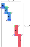 |
Fig. A.1 Matrix X as of Fig. 3 with alternative indexing of the sub-matrices. |
| In the text | |
Current usage metrics show cumulative count of Article Views (full-text article views including HTML views, PDF and ePub downloads, according to the available data) and Abstracts Views on Vision4Press platform.
Data correspond to usage on the plateform after 2015. The current usage metrics is available 48-96 hours after online publication and is updated daily on week days.
Initial download of the metrics may take a while.