| Issue |
A&A
Volume 710, June 2026
|
|
|---|---|---|
| Article Number | A72 | |
| Number of page(s) | 16 | |
| Section | Stellar structure and evolution | |
| DOI | https://doi.org/10.1051/0004-6361/202558276 | |
| Published online | 03 June 2026 | |
The extremely low-luminosity Type Iax SNe 2022ywf and 2023zgx
1
Department of Experimental Physics, University of Szeged, Dóm tér 9, H-6720 Szeged, Hungary
2
HUN-REN-SZTE Stellar Astrophysics Research Group, Szegedi út, Kt. 766, 6500 Baja, Hungary
3
MTA-ELTE Lendület “Momentum” Milky Way Research Group, Szent Imre H. st. 112, 9700 Szombathely, Hungary
4
European Southern Observatory, Alonso de Córdova 3107 Vitacura, Casilla, 19001, Santiago, Chile
5
Department of Physics and Astronomy, Rutgers, the State University of New Jersey, 136 Frelinghuysen Road, Piscataway, NJ 08854, USA
6
Department of Physics and Astronomy, Purdue University, 525 Northwestern Ave, West Lafayette, IN 47907, USA
7
Steward Observatory, University of Arizona, 933 North Cherry Avenue, Tucson, AZ 85721-0065, USA
8
Graduate Institute of Astronomy, National Central University, 300 Jhongda Road, 32001 Jhongli, Taiwan
9
Las Cumbres Observatory, 6740 Cortona Drive, Suite 102 Goleta, CA 93117-5575, USA
10
Department of Physics, University of California, Santa Barbara, CA 93106-9530, USA
11
Astronomical Observatory, University of Warsaw, Al. Ujazdowskie 4, 00-478 Warszawa, Poland
12
Department of Astronomy & Astrophysics, University of California, San Diego, 9500 Gilman Drive, MC 0424 La Jolla, CA 92093-0424, USA
13
Cardiff Hub for Astrophysics Research and Technology, School of Physics & Astronomy, Cardiff University, Queens Buildings, The Parade, Cardiff CF24 3AA, UK
14
Center for Interdisciplinary Exploration and Research in Astrophysics (CIERA), 1800 Sherman Ave., Evanston, IL 60201, USA
15
School of Physics, Trinity College Dublin, The University of Dublin, Dublin 2, Ireland
16
Instituto de Ciencias Exactas y Naturales (ICEN), Universidad Arturo Prat, Iquique, Chile
17
Department of Astronomy, The University of Texas at Austin, 2515 Speedway, Stop C1400 Austin, TX 78712, USA
18
Center for Astrophysics and Cosmology, University of Nova Gorica, Vipavska 11c, 5270 Ajdovščina, Slovenia
19
School of Physics and Astronomy, Monash University, Clayton, Australia
20
OzGrav: The ARC Center of Excellence for Gravitational Wave Discovery, Clayton, Australia
21
Astrophysics sub-Department, Department of Physics, University of Oxford, Keble Road, Oxford OX1 3RH, UK
22
Konkoly Observatory, HUN-REN Research Centre for Astronomy and Earth Sciences, MTA Centre of Excellence, Konkoly Thege Miklós út 15-17 Budapest 1121, Hungary
★ Corresponding author: This email address is being protected from spambots. You need JavaScript enabled to view it.
Received:
26
November
2025
Accepted:
25
February
2026
Abstract
Context. We present the optical follow-up of SNe 2022ywf and 2023zgx, two examples from the Iax subclass of thermonuclear supernova (SN) events. With peak absolute magnitudes of MV = −13.7 and −14.4 mag, respectively, both objects belong to the extremely low-luminosity (EL) population of the class.
Aims. The common origin of SNe in the Iax subclass remains under debate, since the distribution of certain observables may indicate that the extremely low-luminosity explosions form a distinct population. We aim to estimate the physical properties of the two EL objects, including mapping the ejecta structure. We compare the results with the predictions of the pure deflagration model with similar luminosity, as well as with the common features of other SNe Iax.
Methods. We performed spectral tomography on the spectral series of SNe 2022ywf and 2023zgx around their maxima to map the physical properties of the ejecta. Together with the analysis of BgVriz photometry, we studied a wide range of observables to investigate their distribution against luminosity. We compared the constrained chemical abundances of the ejecta to the predictions of hydrodynamic simulations with similar peak luminosities.
Results. Constant abundances provide a good match for the distribution of chemical elements for both SNe 2022ywf and 2023zgx. The discrepancies compared to the least luminous pure deflagration model N5def_hybrid are minor, especially at post-maximum epochs. The two SNe also share similar characteristics in their constrained density structures, as well as in the evolution of the photosphere.
Conclusions. The analysis supports the assumption that pure deflagration models can reproduce the main characteristics of SNe Iax, even for the low-luminosity population. The presented indirect observational evidence indicates that these objects show similar intrinsic properties to the well-studied, relatively luminous Iax sample and fit into the velocity distribution of the subclass.
Key words: radiative transfer / supernovae: general / supernovae: individual: SNe 2022ywf / supernovae: individual: SNe 2023zgx
LSST-DA Catalyst Fellow.
© The Authors 2026
 Open Access article, published by EDP Sciences, under the terms of the Creative Commons Attribution License (https://creativecommons.org/licenses/by/4.0), which permits unrestricted use, distribution, and reproduction in any medium, provided the original work is properly cited.
This article is published in open access under the Subscribe to Open model. This email address is being protected from spambots. You need JavaScript enabled to view it. to support open access publication.
1. Introduction
Type Ia supernovae (SNe) originate from the thermonuclear explosion of C/O white dwarfs (WDs). Although significant exploration has still not confirmed the most probable progenitor and explosion scenario, the remarkable homogeneity of the so-called “normal” SNe makes the Ia class the most important objects for distance estimations Phillips (1993). However, several subclasses of thermonuclear SNe (Taubenberger 2017) indicate that there are multiple channels for degenerate WDs; thus, studying these peculiar explosions provides essential information on SN physics.
The most numerous subclass of thermonuclear SNe is formed by the Iax (or, after their prototype object, “2002cx-like”) SNe. Volume-limited samples of nearby surveys investigated by Foley et al. (2013) indicate a relative rate of  for SNe Iax compared to normal Ia explosions. However, the sample from the recent second data release of the Zwicky Transient Facility (which included ∼3600 and ∼1580 thermonuclear SNe in the total and volume-limited samples, respectively) indicates that the relative rate of SNe Iax is only ∼4.5% Dimitriadis et al. (2025). A possible reason for the discrepancy is that the relative rates of subluminous SNe Ia can be estimated only by assuming correction factors for the lower probability of detection and classification. This correction can be critical for SNe Iax with the lowest peak luminosity and shorter light-curve widths, adding significant uncertainty to population estimates.
The lower peak luminosity of SNe Iax also strongly limits the sample suitable for detailed analysis, in contrast to normal SNe Ia. Since the first classification (SN 2002cx, Li et al. 2003), approximately 110 transients have been identified as type Iax SNe according to WISeREP1, but fewer than 20 of them have published, well-sampled photometric and spectroscopic datasets. The extreme diversity of the subclass hinders the investigation of the nature of type Iax SNe. Their peak absolute magnitude covers a wide range, from relatively luminous objects with a peak absolute magnitude of MR = −18.60 mag (SN 2011ay, Szalai et al. 2015) to extremely faint ones with Mr = −12.66 mag (SN 2019gsc, Karambelkar et al. 2021) in the R/r band. Similarly, other physical characteristics of these SNe also show extremities, such as the decline rate, spectral velocities, or implied ejecta masses.
Multiple mechanisms have been proposed to explain the peculiar nature of Iax explosions. The pure (or “failed”) deflagration scenario is currently considered the most promising concept (for a full review, see Lach et al. 2022). Hydrodynamic simulations (Jordan et al. 2012; Kromer et al. 2013; Long et al. 2014; Fink et al. 2014; Kromer et al. 2015; Leung & Nomoto 2020; Lach et al. 2022) have shown that the diverse physical properties of the sample can be reproduced by scaling the strength of the deflagration of a C/O WD. A common feature in all pure deflagration models is that the kinetic energy is insufficient to fully unbind the WD; thus, the explosion leaves behind a bound remnant. As a further consequence, the ejecta of an SN Iax is expected to have a lower mass and a lower average density than that of normal SNe Ia. However, this scenario cannot account for the least luminous SNe Iax, represented by the prototype SN 2008ha. Kromer et al. (2015) proposed a C/O/Ne WD as a potential progenitor, which successfully decreased the energy produced and, thus, the luminosity of the models. No other pure deflagration model has produced SNe fainter than Mr > −15 mag, while Kromer et al. (2015) presented only one hydrodynamic simulation. Since SN 2008ha, researchers have discovered even less luminous SNe (e.g., SNe 2019gsc, 2021fcg, 2024vjm, Tomasella et al. 2020; Srivastav et al. 2020; Karambelkar et al. 2021; Kwok et al. 2025). For these objects, the double-degenerate merger model presented by Kashyap et al. (2018) reproduces their peak absolute magnitudes and low ejected masses. This scenario produces a failed detonation and provides numerous testable differences compared to failed deflagration, such as strong stratification of chemical elements or relatively higher expansion velocities.
A major breakthrough in understanding SNe Iax came with the discovery of the progenitor system of SN 2012Z (McCully et al. 2014; Stritzinger et al. 2015) in pre-explosion Hubble Space Telescope images of its host, NGC 1309. The luminous blue progenitor suggests that the system included a helium-star donor and an accreting, near-Chandrasekhar-mass WD. If correct, this interpretation confirms that at least some WD SNe originate in the single-degenerate scenario (McCully et al. 2014). In contrast, no luminous companion star has ever been directly observed for a normal SN Ia or for any other SNe Iax.
Therefore, the common origin of the extremities of SNe Iax remains under debate, and most studies divide the subclass into luminosity samples. Srivastav et al. (2022a) use a peak absolute magnitude MV = −16 mag to distinguish the “faint” SNe Iax from the rest of the category. Singh et al. (2023) argue for clustering among SNe Iax, as the “faint” (Mr > −14.6 mag) and “bright” (Mr < −17.1 mag) samples show different correlations between peak luminosity and the Δm15 parameter, which describes post-peak fading. Type Iax SNe with intermediate luminosities range between the two groups presented by Singh et al. (2023) have long been known; however, their low numbers and the lack of observational series make their characterization difficult. The first example with a detailed analysis, SN 2019muj (Barna et al. 2021), shows a transitional nature that bridged the luminosity gap between the faint and bright groups. The constrained intrinsic characteristics (e.g., ejecta mass and expansion velocities) and the spectroscopic evolution imply that most physical properties and observables change continuously throughout the entire Iax subclass, rather than clustering. Recent studies of objects with similar luminosities (SNe 2022xlp and 2024pxl, Bánhidi et al. 2025; Singh et al. 2025, respectively) also support this result. Regardless of whether their origin scenarios differ, labeling various groups of the diverse Iax subclass is useful for referencing objects with different properties. We suggest and hereafter adopt a three-level (sub-)classification:
-
Relatively luminous (RL) group: (Mr < −17 mag), example: SN 2011ay.
-
Intermediate luminous (IL) group: (−14.5 mag > Mr > −17 mag), example: SN 2019muj.
-
Extremely-low luminosity (EL) group: (Mr > −14.5 mag), example: SN 2008ha.
As discussed above, the diverse nature of SNe Iax can only be fully understood by sampling the entire subclass. We present SNe 2022ywf and 2023zgx, both peaking around MV ∼ −14 mag, to further characterize the observables and physical properties, particularly for the lowest-luminosity events of this class. The paper is organized as follows. In Sect. 2, we describe the discovery of the two objects and the properties of their host galaxies, followed by the sources and characteristics of the observed datasets. We introduce the techniques used to analyze the photometric and spectroscopic data in Sects. 3 and 4, respectively, and describe the inferred results. We summarize the conclusions in Sect. 5.
2. Observations
2.1. SN 2022ywf
SN 2022ywf (RA 01:22:12.20, Dec +00:57:23.55) was discovered by the Zwicky Transient Facility (ZTF) at 59880.18 MJD while still on the rise at mr = 19.95 mag, with the last nondetection at 59879.33 MJD with a magnitude limit of 20.4 mag in the g band. The Asteroid Terrestrial-impact Last Alert System program (ATLAS; Tonry et al. 2018) also observed the field of SN 2022ywf, providing a deep 20.7 mag nondetection limit in the cyan band on 59879.19 MJD. The first spectrum obtained at 59881.3 MJD (Bostroem et al. 2022) classified it as a type Ia SN; subsequent data (Srivastav et al. 2022b) later refined this classification to type Iax. The host of SN 2022ywf is NGC 493, an SBc-type galaxy. The distance to NGC 493 has been constrained multiple times using the Tully-Fisher relation. These results converge to 22.0−24.5 Mpc. In the following, we adopt the latest distance estimate of d = 22.8 ± 4.7 Mpc (Tully et al. 2016). The SN appeared 50″ (∼5600 pc) northeast of the host galaxy center. Because of its location in the outskirts of the galactic disk and the nondetection of the Na I D lines at the NGC 493 redshift, we assume negligible host-galaxy reddening.
The ATLAS photometry at the position of SN 2022ywf was obtained through the public forced photometry server2 (Shingles et al. 2021). In addition to the measured fluxes (in μJy) and associated errors, the forced photometry server also provides quality metrics, including a reduced chi-squared for the point spread function (PSF) fitting (labeled chi/N). We rejected individual measurements with errors greater than 150 μJy, together with measurements with chi/N > 3. The ATLAS survey typically obtains 4 × 30 s exposures spaced within ∼1 h. We combined each set of four individual measurements that passed the quality cuts defined above into a single measurement using a weighted stacking recipe following Srivastav et al. (2023). We considered stacked measurements with 3σ significance as detections and derived AB magnitudes using 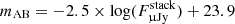 . We converted nondetections into 3σ upper limits using
  .
.
The Las Cumbres Observatory (LCO) initiated follow-up at 59880.8 MJD, providing BgVri light curves (LCs) obtained with multiple 1-m telescopes (Brown et al. 2013) located at Sutherland (South Africa), CTIO (Chile), Siding Spring (Australia), and McDonald (USA) observatories, through the Global Supernova Project (GSP). After +30 days, BV LCs showed highly scattered and uncertain magnitudes, but we include gri data until 59984 MJD, when photometric monitoring ceased (Table A.3). The ATLAS survey followed SN 2022ywf in c and o bands. The first detection occurred at 59880.45 MJD (mc = 19.60 ± 0.14 mag) and was regularly observed until 59931.6 MJD, when the target faded below the detection limit (Table A.1). Fig. 1 shows the ATLAS o- and c-band LCs of SN 2022ywf, while Fig. 2 compares its BgVri photometry with that of SN 2023zgx.
 |
Fig. 1. ATLAS photometry of SNe 2022ywf and 2023zgx. The observation dates of SN 2023zgx are shifted 400 days earlier. The dashed red line show the fit of Eq. (1) to the pre-maximum o-band data of SN 2022ywf. |
We obtained optical spectroscopy of SN 2022ywf with the 9.2-m Southern African Large Telescope (SALT) and the Robert Stobie Spectrograph (RSS) through the Rutgers University program. The LCO obtained optical spectra with FLOYDS spectrographs mounted on the 2-m Faulkes Telescope North and South at Haleakala (USA) and Siding Spring (Australia) through the GSP. We obtained three spectral epochs with the Low Resolution Spectrograph 2 (LRS2) (Chonis et al. 2014) mounted on the Hobby-Eberly Telescope (HET, Ramsey et al. 1998) at McDonald Observatory. We obtained two spectra with the Southern Astrophysical Research (SOAR) telescope using the red camera of the Goodman High-Throughput Spectrograph (GHTS; Clemens et al. 2004) and were reduced using the Goodman Pipeline3. We obtained additional spectra from the KOSMOS medium resolution spectrograph on the Apache Point Observatory (APO) ARC 3.5m telescope (); the Boller and Chivens (B&C) spectrograph on the University of Arizona’s Bok 2.3m telescope located at Kitt Peak Observatory; the ESO Faint Object Spectrograph and Camera version 2 (EFOSC2; Buzzoni et al. 1984) at the 3.6-m New Technology Telescope (NTT) in the frame of the ePESSTO+ collaboration (Smartt et al. 2015); and the SPRAT low resolution spectrograph on the Liverpool Telescope (LT). Fig. 3 shows all optical spectra of SN 2022ywf.
2.2. SN 2023zgx
Koichi Itagaki discovered SN 2023zgx (RA 12:44:05.00, Dec −05:40:53.47) at 60287.8 MJD, likely a few days before its peak, at a visual brightness of 16.9 mag. The classification spectrum (Crimes et al. 2023), obtained four days later, identified the transient as a faint type Iax SN; photometric follow-up began during its decline. SN 2023zgx is associated with the DDO 142 S-type galaxy. The only distance estimate, apart from the Hubble-flow, gives 25.4 ± 5 Mpc (Tully & Fisher 1988), which we adopt in this study. This distance is higher than that derived from the redshift of 0.0047 (dz = 20.2 Mpc) but remains consistent with it. SN 2023zgx was also monitored by LCO sites, providing BgVri LCs between 60294.7 and 60378.2 MJD.
The Gemini Multi-Object Spectrograph mounted at Gemini North (GMOS-N; Hook et al. 2004) obtained the first spectrum of SN 2023zgx two days before the start of the photometric monitoring. The ePESSTO+ collaboration (Smartt et al. 2015) initiated spectroscopic follow-up using EFOSC2/NTT and GSP with multiple LCO/FLOYDS spectrographs. We obtained late-time (t + 80 days) spectra with SALT/RSS between +80 and +90 days after the r-band maximum.
Table A.5 lists the observed BgVriz photometry of SN 2023zgx and Fig. 4 shows the reduced spectra, corrected for host-galaxy redshift. For further analysis, we scaled all spectra to photometry using polynomial functions and dereddened for Milky Way extinction.
3. Photometric analysis
For SN 2022ywf, the photometric coverage was sufficient to fit a low-order polynomial function to the LCs of each filter around the maximum, extending to +20 days. Table 1 lists the inferred parameters, including the peak magnitude and Δm15 decline rate. Using a distance modulus of μ = 31.79 mag distance modulus and accounting for Milky Way reddening (assuming no host-galaxy reddening based on the absence of Na I D lines) the peak absolute magnitude of SN 2022ywf is Mr = −13.81 ± 0.44 mag, placing the object in the EL group of the Iax subclass. Based on their peak luminosities, the closest relatives to SN 2022ywf are SNe 2008ha and 2019gsc. The polynomial fits yield Tmax = 59890.4 MJD for the r-band maximum, which we used as a further reference date, as in our previous works.
Light-curve parameters of SN 2022ywf.
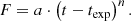
The ATLAS co-band LCs provide early detections supplemented with deep nondetection limits (> 20.7 mag). We fit the steeply rising early part of the SN LCs with the simple fireball model (Riess et al. 1999), assuming a constant photospheric temperature (Teff) and velocity (vphot); In this model, the emergent flux follows a quadratic function of the time since the explosion (F ∼ texp). Firth et al. (2015) showed that these assumptions are not robust for a large sample of normal Ia SNe, and the early rise of the LC can be fit with a power-law function,
 (1)
(1)
The n exponent, referred to as the rise index, ranges from 1.5 to 2.5, with a mean value of n = 2.44. For subluminous Type Iax SNe, the fit of the rise index is typically lower. Magee et al. (2025) recently studied the rising curves of all available SNe Iax with detailed pre-maximum coverage and found that their rise indices exhibit similar scattering to normal SNe Ia, but with a lower mean value of 1.4−1.5 in the g and r bands. Their sample was mainly limited to the RL group but also included the faintest type Iax SN 2024vjm (ML = −13.19 ± 0.15 mag), for which they report a rise index of 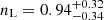 . Similar analyses of individual SNe show that the least luminous objects (e.g., SNe 2015H, 2019muj and 2020udy, Magee et al. 2016; Barna et al. 2021; Singh et al. 2024, respectively) have rise indices n < 1.3, a possible link between luminosity and rise parameters of type Iax SNe.
Treating the rise index as a free parameter when fitting the SN 2022ywf o-band LC (see Fig. 1), which includes the most pre-maximum observations, yields an extremely low exponent (n = 0.38 ± 0.09) and might be an unrealistic first-light date (T0 = 59880.25 ± 0.22 MJD), coinciding with the discovery time (59880.17 MJD). This inconsistency likely results from insufficient coverage of the rising phase, with six pre-maximum observations in the o band and even fewer in other filters. Therefore, we assumed the time of first light based on the last nondetection and the first detection in the c band as T0 = 59879.8 ± 0.6 MJD.
As an alternative estimate of T0, and hence the rise time, the abundance tomography analysis (see Sect. 4.1) provides constraints on the time of first light, as the spectral time series fit includes the input parameter texp as the dilution factor of the density structure. However, the constrained densities correspond to the explosion date, which precedes the escape of the first photons from the ejecta, i.e., first light. The interim period, also called the dark phase, may cover a few days for SNe Ia (Piro & Nakar 2013) and for explosion models with a compact 56Ni distribution (Magee et al. 2020). By contrast, deflagration models predict dark phases shorter than one day (Fink et al. 2014).
SN 2023zgx, the other subject of this study, peaks at around −14.4 mag in the r band, based on similarities with SN 2022ywf in post-maximum LCs and spectral evolution (see Fig. 2). The same set of photometric parameters cannot be precisely estimated due to sparce pre-maximum coverage. However, the many similarities between the two SNe suggest that we can safely assume a similar LC evolution and constrain the time of peak brightness of SN 2023zgx based on that of SN 2022ywf. The declining LCs in the g, V, and r-bands can be aligned with those of SN 2022ywf in the first two weeks after maximum by assuming a shift of Δt = T23zgx(rmax)−T22ywf(rmax) = 400 days along the time axis (see Fig. 2) and Δmr = +0.2 mag along the magnitude axis. Applying the same Δt provides an excellent match with the ATLAS c and o band LCs of the two SNe with a slightly larger shift in brightness (Δmo = 0.5 mag). From the LC shift match, we adopt T23zgx(rmax) = 60290.4 MJD as an approximate date of maximum for SN 2023zgx, which we use hereafter as the reference epoch, with an approximate uncertainty of ±3 days. The LC comparison suggests that SN 2023zgx fades more slowly; however, this conclusion is mainly supported by the photometry after +20 days, when observations of SN 2022ywf become uncertain. The decline rates show significant differences in the B and i filters, suggesting a different color evolution for the two objects. The lack of pre-maximum photometry for SN 2023zgx limits the determination of the explosion date. The abundance tomography analysis described in Sect. 4 constrains the quantitative estimates of Texp.
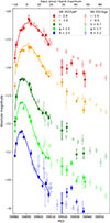 |
Fig. 2. Ground-based photometry of SNe 2022ywf (filled circles) and 2023zgx (fainter diamonds). The horizontal axis shows the observational dates of SN 2022ywf in MJD. For SN 2023zgx, the data points are shifted 400 days earlier for better comparison. The LC fits with fourth-order polynomial functions are also shown for SN 2022ywf (solid lines). |
4. Spectral analysis
Figures 3 and 4 show the optical spectra of SNe 2022ywf and 2023zgx, respectively. Due to the short sampling period of SN 2022ywf and the lack of pre-maximum epochs for SN 2023zgx, the two spectral series overlap in phase for only a few days. The three spectra of SN 2023zgx obtained during this period show excellent agreement with those of SN 2022ywf, which underlines the general similarity of the intrinsic properties of the two objects. SN 2022ywf evolves slightly faster, evident from the shifting epochs of the matching spectra. This may result from a shorter diffusion timescale due to a lower ejecta mass, which can be tested by comparing the inferred density profiles from abundance tomography (see below).
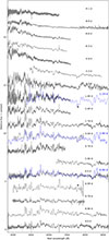 |
Fig. 3. Optical spectra of SN 2022ywf. Epochs show days relative to r-maximum. Table A.4 lists the observation log. The first three spectra of SN 2023zgx (blue) are shown for comparison to SN 2022ywf spectra (gray) at similar phases. |
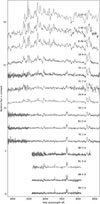 |
Fig. 4. Optical spectra of SN 2023zgx. Epochs show days relative to r-maximum. Table A.6 lists the observation log. |
We analyzed the first 20 days of the spectral time series of SNe 2022ywf and 2023zgx sampled with seven and four spectra, respectively, obtained at pre- and near-maximum epochs. During this period, the assumptions of TARDIS (Kerzendorf & Sim 2014), such as the existence of a sharp photosphere, are robust, allowing rapid modeling of realistic synthetic spectra in the optical regime. We fit these spectral time series, listed in Tables A.4 and A.6, following the method of abundance tomography analysis. This technique assumes that line formation occurs mainly near the photosphere; thus, each spectral epoch constrains a specific layer of the ejecta. The retreating photosphere enables mapping of the ejecta inward by fitting the spectral time series. Later epochs also probe the outer layers, as some chemical elements form lines in the more dilute, cooler regions of the ejecta.
Multiple studies have performed abundance tomography of SNe Iax since the first adaptations (Magee et al. 2016; Barna et al. 2017) of the TARDIS radiative transfer code (Kerzendorf & Sim 2014). The rapid evolution of the optical spectra, together with the numerous unblended spectral features that are not saturated compared to those of normal SNe Ia, provides suitable conditions for fitting a large number of ejecta parameters through rapid modeling with a simplified radiative transfer code. Multiple studies have performed similar abundance tomography on SNe 2002cx, 2005hk, and 2012Z (Barna et al. 2018); 2019gsc (Srivastav et al. 2020); 2019muj (Barna et al. 2021); 2018cni and 2020kyg (Singh et al. 2023); and 2020udy (Singh et al. 2024), constraining density profiles, abundance ratios, photospheric properties, and explosion (the exact fitting strategy varies between studies; for more details, see the references). It is important to note that none of these modeling attempts aimed to find the best fit due to the large number of fitting parameters. Instead, our fitting process provides a feasible solution for the model atmosphere (labeled as “best-fit” for simplicity) by testing and modifying the results of the N5def_hybrid (Kromer et al. 2015) pure deflagration model.
4.1. SN 2022ywf
As a first approach, we reduce the number of free parameters by adopting constant abundances based on the predictions of a corresponding deflagration model, similar to the analysis of SN 2014dt described by Camacho-Neves et al. (2023). Considering the peak luminosities, the only hydrodynamic simulation with MV ∼ 14 mag is N5def_hybrid, assuming the failed deflagration of a CONe-hybrid WD. The estimated observables of the hydro model show a good match with the early photometric and spectroscopic evolution of the EL-Iax SN 2008ha, but it fails to reproduce the decline rate and the continuum flux weeks after the maximum. The adopted constant chemical composition based on the N5def_hybrid (see Fig. 8) is characterized by C, O, 56Ni, and stable iron-group elements (IGEs), mostly Fe, as the most abundant elements, each with a mass fraction of approximately 20%. Despite adopting this uniform chemical structure, we fit the continuum and the line widths at each epoch, allowing us to constrain ρ(v), texp and vphot, whose parameters affect the local temperature of the ejecta at the first approximation.
For the density structure, we adopted a purely exponential function similar to that of N5def_hybrid:
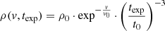 (2)
(2)
where ρ0 is the central density at t0 reference time (typically chosen as texp = 100 s, the approximate end of the fusion processes and the beginning of homologous expansion). The parameter v0 characterizes the slope of the density profile. This model does not exhibit any cutoff in the outer layers, unlike the similarly constrained density profiles of RL SNe (Barna et al. 2018) and the corresponding hydrodynamic models (Fink et al. 2014). Because the studied spectral series does not cover the vast majority of the ejecta, we cannot constrain the ejecta mass Mej from abundance tomography; only the bolometric LC fitting can provide such an estimate. However, the fitted parameters of Eq. (2) allow a quantitative comparison between the outer layers of other SNe Iax and deflagration models.
The fit of the density structure is relatively uncertain because the two main properties defining the function, the ρ0 central density and the v0 slope of the exponential function, are strongly coupled. The segment of the density function sampled by a given spectral epoch mainly affects the optical depth of the lines but also influences the temperature profile of the ejecta, allowing us to constrain the densities. During the fitting process, we found that TARDIS modeling is sensitive to density changes of at least 50%, as such changes produce discrepancies in the observed spectral features that cannot be compensated for by modifying chemical abundances or other physical parameters. Fig. 7 shows the density function used for the SN 2022ywf model.
Compared to the other two fitting parameters, the explosion date can be fit precisely since it affects the entire spectral time series through the dilution of the density profile (see texp in Eq. 2). The best-fit value is Texp = 59878.4 MJD. The early epochs, particularly the first three between texp = 3.1 and 5.7 days, are very sensitive to Texp because even a few hours can strongly modify the temperature profile and the continuum. Although our method is not suitable for detailed uncertainty analysis, the estimated upper limit for the error in Texp is ±0.5 day. This implies a dark phase between the first light and the explosion of T0 − Texp = 1.4 days.
Next, we allowed the constant mass fractions of elements that significantly affect the spectral features (C, Mg, Si, S, Ca, Fe, and the most abundant radioactive isotope, 56Ni) to vary. The TARDIS code uses the actual decay state products at each epoch; therefore, the abundances of Co and Fe increase with time. Other elements and isotopes, such as Ne, although relatively abundant (X(Ne)≃0.03), have a limited impact on the early optical evolution, so we kept their initial mass fraction fixed. We used oxygen as a buffer element to normalize the total mass fraction of chemical elements to 1. Furthermore, the features of post-maximum epochs indicate the inclusion of Cr and V, two elements that may originate from the radioactive decay of 54Fe but are expected to be present at low abundances. We added the required mass fractions (X(Cr)≃0.01; X(V)≃0.001) to the models at each epoch to maintain a uniform chemical structure, despite a slight deterioration of the fit in the early epochs (i.e., in the outer region of the ejecta). This behavior implies a stratified distribution of these elements.
The best-fit ejecta model contains only constant chemical mass fractions, similar to the abundance structure of the N5def_hybrid model used for the initial input. This simplification allowed us to treat the abundances of the aforementioned elements as free parameters. The synthetic spectra of our best-fit model successfully reproduce all prominent features throughout the studied three-week time span (see Fig. 5). Inconsistencies, such as shifts of certain spectral lines, arise from the simplifications of the fitting method and/or the limitations of the radiative transfer code.
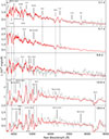 |
Fig. 5. Five spectral epochs of SN 2022ywf (gray) fit with the TARDIS synthetic spectra (red) from the abundance tomography analysis. |
These mismatches involve shifted synthetic lines, which may result from the incorrect assumption of constant abundances. The C II λ6580 lines show a consistent redshift relative to the observations, suggesting that some carbon stratification may be necessary in the outer layers of the ejecta. Another shortcoming of the synthetic spectra is the absence of several features between 6000 and 8300 Å after maximum, which appear as narrow P Cygni lines and were previously identified as C II and Fe II features (Tomasella et al. 2016). Because the strong iron features formed near the photosphere are relatively well reproduced at texp = 14.8 and 18.0 days, and both X(C) and X(Fe) remain constant throughout the model atmosphere, this issue likely originates from the outer, cooler region of the model ejecta.
We modified the Si and S mass fractions by a few percentage points to improve the fits of the characteristic spectral features λ6345 and λ5607, respectively. We modified the fractions of two low-abundance elements, Ca and Cr, by factors of ∼3 to fit the short-wavelength end of the spectra and reproduce characteristic post-maximum spectral features, namely Cr II λ5276 and the Ca II NIR triplet. However, these discrepancies in the N5def_hybrid hydro model are not significant, as the adjustments affect only a few tenths of a percentage point. The main differences arise in IGE abundances, as both radioactive Ni and stable Fe have significantly lower mass fractions in our model. Fig. 5 shows that these updates reproduce the corresponding lines in the two earliest spectra. However, even reducing both X(Fe) and X(56Ni) mass fractions by ∼0.12 produces excessively strong Fe III λ4420, λ5157, and Ni II λ4068 lines for the spectrum at texp = 3.1 days, but provides a relatively good match for the spectral features at texp = 5.7 and 9.8 days. This inconsistency results from the use of a uniform chemical structure, since the outer ejecta of SNe Iax may have even lower IGE abundances.
4.2. SN 2023zgx
The spectral series of SN 2023zgx covers a significantly longer period, almost three months of spectral evolution. Although type Iax SNe never become fully nebular, the radiative transfer code assuming a sharp photosphere can reproduce part of the optical regime (Camacho-Neves et al. 2023); however, the emergence of forbidden lines limits the quality of the fit. Consequently, and for consistency with the fitting of SN 2022ywf, we fit only the first four epochs (approximately the first five weeks after the explosion) of the spectral series. We repeated the fitting process using the same principles; however, in contrast to the case of SN 2022ywf, fewer fitting constraints were available due to the lack of early spectra sampling the outermost regions of the ejecta. This limitation makes the physical parameters more uncertain, particularly regarding layers over 5000 km s−1, which are already distant from the photosphere at the first epoch.
Fitting only the post-maximum epochs of SN 2023zgx, its chemical composition is less constrained. This is in part because synthetic spectra generally become less sensitive to changes in mass fractions over time. Moreover, weaker lines cannot be well constrained due to the presence of strong, overlapping Fe II features. Thus, the distribution of chemical elements that significantly affect pre-maximum spectral features, such as C, S, and Ni, can be effectively described by the mass fractions of the N5def_hybrid model, used as initial input.
Despite delayed follow-up, tomography analysis investigated the same velocity coordinates as those of SN 2022ywf because SN 2023zgx has lower expansion velocities. The slopes of the inferred ejecta structures of the two SNe are similar, but the layers at the same velocities are denser in the SN 2023zgx model to reproduce the strong post-maximum IGE features. This may also explain the higher photospheric velocities of SN 2023zgx at the same epochs, regardless of whether they are relative to the maximum or the moment of explosion. This relation aligns with trends in deflagration models, where more energetic and luminous explosions produce more massive ejecta with higher densities, even in the outer regions (Fink et al. 2014; Lach et al. 2022) The angle-averaged density function of N5def_hybrid agrees reasonably well with the best SN 2023zgx model above 3000 km s−1, but it exceeds it considerably in deeper ejecta.
The explosion time is also more uncertain because texp mainly impacts the spectrum through density dilution. For early-epoch fits, the explosion date can be constrained to approximately ±1 day, but the synthetic spectra of SN 2023zgx are relatively insensitive to changes of ∼2 days in texp due to the lack of pre-maximum spectra. The tomography analysis constrained the explosion date to Texp = 60276.1 MJD, yielding a rise time comparable to that of SN 2022ywf.
The best-fit synthetic spectra provided (see Fig. 6) show a good match to the observations, as almost all prominent lines are present with at appropriate optical depths. We also added a high Na abundance to the model ejecta to fit the growing feature around 5800 Å, which becomes one of the most prominent P Cygni features at texp = 33.2 days, consistent with late-time spectral synthesis of SNe 2014dt and 2022xlp (Camacho-Neves et al. 2023; Bánhidi et al. 2025, respectively). The only striking difference is in the Ca II NIR triplet, where rising forbidden-line emission disrupts the fitting based on the photospheric assumptions. Another limitation of the fit is that the Fe II lines between 4200 and 5400 Å are too strong, resulting from Fe in the outer regions of our model ejecta. The flux continuum is also well-reproduced for all four spectra, indicating reasonable estimates of the photospheric velocity and density profile (including texp). Compared to SN 2022ywf, the post-maximum spectral evolution of SN 2323zgx is better reproduced under the adopted assumptions, indicating a uniform abundance structure for the inner regions of the ejecta.
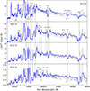 |
Fig. 6. Four spectral epochs of SN 2023zgx (gray) fit with the TARDIS synthetic spectra (blue) from in the abundance tomography analysis. |
Table 2 lists the constrained ejecta parameters of the best-fit TARDIS models. Figs. 7 and 8 show the density structures and chemical abundances of SN 2022ywf, together with those of SN 2023zgx. We note that our fitting strategy was designed to test the predictions of the corresponding hydrodynamic model N5def_hybrid; therefore, the differences between the ejecta models of SNe 2022ywf and 2023zgx may not be real. We obtained the constant chemical structure based on the N5def_hybrid model with modified iron (X(Fe) = 0.025), chromium (X(Cr) = 0.01), and sodium (X(Na) = 0.07) abundances. These modifications are largely consistent with the constrained model atmosphere of SN 2022ywf. Furthermore, the abundance structure of SN 2022ywf would provide an equally good fit for SN 2023zgx. This implies that abundances differing from N5def_hybrid to fit the early spectral features of SN 2022ywf (e.g., decreased carbon and nickel mass fractions) have minimal impact on spectral formation at post-maximum epochs.
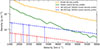 |
Fig. 7. Exponential functions assumed for the density profiles of SNe 2022ywf (red) and 2023zgx (blue) in the best ejecta models, scaled to texp = 100 s. The density structures of the two least-luminous pure deflagration models are shown for comparison. Vertical lines indicate the photosphere location at the epochs used in the corresponding models. |
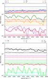 |
Fig. 8. Mass fractions of chemical elements from the abundance tomography analysis of SNe 2022ywf (dashed lines) and 2023zgx (dotted lines). The chemical abundances of the pure deflagration model N5def_hybrid (solid lines) are shown for comparison. The mass fractions of radioactive 56Ni are scaled to texp = 100 s. |
Physical parameters of the best-fit TARDIS models for SNe 2022ywf and 2023zgx.
4.3. Comparison with other extremely faint SNe Iax
To date, only five SNe Iax from the faintest end of the subclass luminosity range (i.e., with MV < 14 mag) have been published with detailed follow-up observations before and around maximum light. In this section, we compare the optical spectral evolution and features of SNe 2022ywf and 2023zgx with those of the faint Iax objects: SNe 2008ha (Foley et al. 2009), 2020kyg (Singh et al. 2024), 2019gsc (Srivastav et al. 2020; Tomasella et al. 2020) and 2021fcg (Karambelkar et al. 2021).
Figure 9 shows the spectral epochs before the r-band maximum and approximately ten days afterward. Although the EL sample shares some common features in their spectral evolution, such as the presence of the Si II λ6355 and the C II λ6580 lines, the strength of these spectral features vary significantly between objects with similar luminosities. These differences are amplified for the post-maximum epoch, when SN 2008ha shows broad IGE absorption, whereas SN 2022ywf shows a more typical set and appearance of P Cygni lines, similar to SN 2005hk. SN 2019gsc, in contrast, lacks strong (pseudo-)emission peaks and shows a significantly slower spectral evolution over 16 days. Since the identified lines are similar, the variation in spectral features may be attributed to differences in ejecta temperatures. This idea is supported by the color evolution and consequently the continuum evolution of the compared objects. Whereas the ejecta temperature of SN 2019gsc changes little between the epochs in this comparison, SN 2022ywf cools from a hotter ejecta to a cooler phase, transforming the initial presented Fe III and Ni III features into a Fe II-dominated post-maximum epoch. The more rapid cooling of SN 2022ywf can be linked to a steeper density gradient, potentially resulting from either the different ejecta mass or a line-of-sight effect, which provides insight into a less dense region of the SN.
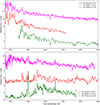 |
Fig. 9. Spectral comparison of three SNe Iax from the EL sample at similar epochs. The spectra are corrected for reddening and redshift; epochs are taken from the corresponding publications of SNe 2008ha (Foley et al. 2009; Valenti et al. 2009) and 2019gsc (Srivastav et al. 2020). |
Several studies have investigated correlations between the peak luminosities of SNe Iax and other observable properties. Singh et al. (2023) and Magee et al. (2025) presented a correlation between the rise time (trise) and the peak absolute magnitude in the r band, with brighter SNe Iax typically reaching their maximum later. However, this correlation remains ambiguous due to the limited sample and the high uncertainties in the estimated parameters trise, resulting from the relatively late discoveries. The decline parameter Δm15, which shows a greater variance, instead suggests clustering, where brighter and fainter samples appear to behave differently (Singh et al. 2023). The absence of strong correlations and the continuous distribution of physical properties across the luminosity range suggest that not all transients classified as type Iax SNe originate from the same explosion scenarios.
Multiple studies have also discussed a potential correlation between peak luminosity and expansion velocity. Tomasella et al. (2016) investigated a small sample of SNe Iax with spectral coverage around their maximum and constrained vphot values. They found no evidence that higher-velocity SNe Iax have lower peak absolute magnitudes, as the trend among five objects was disrupted by two outliers, SNe 2009qu (Narayan et al. 2011) and 2014ck (Tomasella et al. 2016), with higher velocities than expected. We note that these statistics rely on vphot values that were sometimes estimated inconsistently. The standard method for calculating the current location of the photosphere, as adopted from the analysis of normal SNe Ia, is based on the blueshift of the absorption feature of the prominent Si II line. Multiple studies (Szalai et al. 2015; Maguire et al. 2023) demonstrate that this method is unreliable for SNe Iax because the λ6355 feature overlaps with Fe II absorption, even at pre-maximum epochs. Barna et al. (2021) report a stronger trend between peak luminosity and vphot estimated at the moment of B-band maximum light, when the velocities are constrained by abundance tomography. The tomography analysis using a radiative transfer code not only ensures consistency when comparing different SNe Iax but also fits the continuum flux and various spectral lines simultaneously. This allowed us to constrain the bottom of the line-forming regions simultaneously and avoids incorrect fits due to the line misidentification, providing a more certain estimate of vphot.
Figure 10 compares the vphot evolution of SNe 2022ywf and 2023zgx with that of other EL SNe Iax. The vphot curves plotted as a function of texp do not intersect, supporting the assumption that the relationship between peak luminosity and expansion velocity extends even to the extremely low-luminosity range of the subclass. For comparison, Fig. 11 shows the relationship of the two physical properties at r-band maximum for all SNe Iax with well-studied spectral series. We include only those cases where the velocity evolution was mapped by spectral synthesis of radiative transfer codes and had coverage around the maximum light. Assuming monotonically decreasing vphot for these epochs, we interpolated to calculate the velocity value for the moment of r- (or, if missing, R-)band maximum. These conditions limit the sample to 13 SNe, covering almost the entire luminosity range of the subclass, with gaps in the IL group. The apparent strong correlation between peak luminosities and expansion velocities further supports the assumption that all SNe Iax, including RL, IL, and EL, share a similar origin. Moreover, the trend is inconsistent with the scenario of a WD merger resulting in failed detonation, since the simulation predicts relatively high photospheric velocities in the case of an even less luminous SN (MV = −11.3 mag, vphot = 3900 km s−1 Kashyap et al. 2018). We note that the estimation of vphot values in Fig. 11 also required distances and is not fully independent of the constrained luminosities. Thus, the assumed correlation requires further investigation.
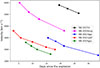 |
Fig. 10. Photospheric velocity evolution of EL and IL SNe Iax constrained by the abundance tomography method. |
 |
Fig. 11. Absolute r/R-band magnitudes of SNe Iax versus photospheric velocity at maximum light. Only SNe Iax with abundance tomography are plotted. In case of no spectral coverage of the maximum (SNe 2015H and 2023zgx), we estimated photospheric velocity via linear extrapolation. Table A.7 lists the corresponding references. |
5. Conclusions
We have presented the photometric and spectroscopic dataset of two SNe Iax from the extremely low-luminosity (EL) regime of the subclass. SN 2022ywf has the most detailed spectroscopic follow-up in the EL sample to date, including multiple pre-maximum epochs; however, monitoring ended two weeks after the r-band maximum. Observations of SN 2023zgx began only after its peak, but the follow-up covers ∼100 days. This study focuses on the first month after explosion, when the photospheric assumption is relatively robust for SNe Iax and the observations of the two objects overlap.
A comparison of the spectroscopic datasets shows that the first three epochs of SN 2023zgx (between +1.4 and +7.1 days) fit the spectra of SN 2022ywf almost perfectly. However, these epochs suggest a slightly faster evolution for SN 2022ywf, possibly related to the steeper ejecta density gradient. Similar conclusions are supported by comparisons with other EL SNe Iax with similar spectral epochs.
The spectroscopic time series of SNe 2022ywf and 2023zgx were analyzed using abundance tomography, which allowed us to map the ejecta properties of both objects.
-
Comparison of the observables with other EL objects reveals differences in post-maximum LC and color evolution.
-
The density structures inferred from abundance tomography for SNe 2022ywf and 2023zgx are comparable to those of the N5def_hybrid model and therefore to each other. Given their lower peak luminosities relative to pure deflagration models, the lower densities are consistent with expectations.
-
The derived uniform abundance models are also consistent with the predictions of the deflagration models, but show slightly lower IGE mass fractions.
-
The photospheric evolution of both studied SNe fits into the general trend of type Iax SNe, as the more luminous objects tend to show higher velocities at the same epochs.
Our analysis of SNe 2022ywf and 2023zgx reveals that the evolution of extremely low-luminosity objects can be efficiently described by the general properties of pure deflagration models, such as constant chemical abundances and steep density profiles. These results support the assumption that, despite the diversity in observables, the EL Iax SNe share the same origin. More broadly, these intrinsic similarities can be extended to all SNe Iax. We show that the correlation between the peak absolute magnitude and the expansion velocity at maximum light may also extend to the EL group. The continuous distribution of certain physical properties across the luminosity range of the subclass makes it probable that all SNe Iax originate from similar explosion scenarios.
Data availability
All spectra of SNe 2022ywf and 2023zgx presented in this study are available via WISeREP online supernova database: https://www.wiserep.org/object/21939 and https://www.wiserep.org/object/24477, respectively.
Acknowledgments
This work uses data from the Las Cumbres Observatory Global Telescope network. The LCO team is supported by NSF grants AST-2308113 and AST-1911151. Based on observations collected at the European Organisation for Astronomical Research in the Southern Hemisphere, Chile, as part of ePESSTO+ (the advanced Public ESO Spectroscopic Survey for Transient Objects Survey – PI: Inserra). ePESSTO+ observations were obtained under ESO program IDs 108.220C and 112.25JQ. This project has received funding from the HUN-REN Hungarian Research Network. B.B. received support from the Hungarian National Research, Development and Innovation Office grants OTKA PD-147091. T.-W.C. acknowledges the financial support from the Yushan Fellow Program by the Ministry of Education, Taiwan (MOE-111-YSFMS-0008-001-P1) and the National Science and Technology Council, Taiwan (NSTC grant 114-2112-M-008-021-MY3). T.E.M.B. is funded by Horizon Europe ERC grant no. 101125877. Time-domain research by the University of Arizona team and D.J.S. is supported by National Science Foundation (NSF) grants 2108032, 2308181, 2407566, and 2432036 and the Heising-Simons Foundation under grant #2020-1864. T.P. acknowledges the financial support from the Slovenian Research Agency (grants I0-0033, P1-0031, J1-8136, J1-2460 and Z1-1853). KAB is supported by an LSST-DA Catalyst Fellowship; this publication was thus made possible through the support of Grant 62192 from the John Templeton Foundation to LSST-DA. Supernova research at Rutgers University is supported in part by NSF grant AST-2407567. SWJ also gratefully acknowledges support from a Guggenheim Fellowship. KAB is supported by an LSST-DA Catalyst Fellowship; this publication was thus made possible through the support of Grant 62192 from the John Templeton Foundation to LSST-DA. J.V. is supported by the NKFIH-OTKA Grant K142534.
References
- Bánhidi, D., Barna, B., Szalai, T., et al. 2025, A&A, 703, A64 [NASA ADS] [CrossRef] [EDP Sciences] [Google Scholar]
- Barna, B., Szalai, T., Kromer, M., et al. 2017, MNRAS, 471, 4865 [NASA ADS] [CrossRef] [Google Scholar]
- Barna, B., Szalai, T., Kerzendorf, W. E., et al. 2018, MNRAS, 480, 3609 [NASA ADS] [CrossRef] [Google Scholar]
- Barna, B., Szalai, T., Jha, S. W., et al. 2021, MNRAS, 501, 1078 [Google Scholar]
- Bostroem, K. A., Valenti, S., Sand, D. J., et al. 2022, Transient Name Server Classification Report, 2022-3154, 1 [Google Scholar]
- Brown, T. M., Baliber, N., Bianco, F. B., et al. 2013, PASP, 125, 1031 [Google Scholar]
- Buzzoni, B., Delabre, B., Dekker, H., et al. 1984, The Messenger, 38, 9 [NASA ADS] [Google Scholar]
- Camacho-Neves, Y., Jha, S. W., Barna, B., et al. 2023, ApJ, 951, 67 [NASA ADS] [CrossRef] [Google Scholar]
- Chonis, T. S., Hill, G. J., Lee, H., Tuttle, S. E., & Vattiat, B. L. 2014, Proc. SPIE, 9147, 91470A [Google Scholar]
- Clemens, J. C., Crain, J. A., & Anderson, R. 2004, SPIE Conf. Ser., 5492, 331 [NASA ADS] [Google Scholar]
- Crimes, A., Levan, A., Leloudas, G., et al. 2023, Transient Name Server Classification Report, 2023-3247, 1 [Google Scholar]
- Dimitriadis, G., Burgaz, U., Deckers, M., et al. 2025, A&A, 694, A10 [NASA ADS] [CrossRef] [EDP Sciences] [Google Scholar]
- Fink, M., Kromer, M., Seitenzahl, I. R., et al. 2014, MNRAS, 438, 1762 [NASA ADS] [CrossRef] [Google Scholar]
- Firth, R. E., Sullivan, M., Gal-Yam, A., et al. 2015, MNRAS, 446, 3895 [NASA ADS] [CrossRef] [Google Scholar]
- Foley, R. J., Chornock, R., Filippenko, A. V., et al. 2009, AJ, 138, 376 [NASA ADS] [CrossRef] [Google Scholar]
- Foley, R. J., Challis, P. J., Chornock, R., et al. 2013, ApJ, 767, 57 [Google Scholar]
- Hook, I. M., Jørgensen, I., Allington-Smith, J. R., et al. 2004, PASP, 116, 425 [NASA ADS] [CrossRef] [Google Scholar]
- Jordan, G. C., Perets, H. B., Fisher, R. T., & van Rossum, D. R. 2012, ApJ, 761, L23 [NASA ADS] [CrossRef] [Google Scholar]
- Karambelkar, V. R., Kasliwal, M. M., Maguire, K., et al. 2021, ApJ, 921, L6 [NASA ADS] [CrossRef] [Google Scholar]
- Kashyap, R., Haque, T., Lorén-Aguilar, P., García-Berro, E., & Fisher, R. 2018, ApJ, 869, 140 [NASA ADS] [CrossRef] [Google Scholar]
- Kerzendorf, W. E., & Sim, S. A. 2014, MNRAS, 440, 387 [NASA ADS] [CrossRef] [Google Scholar]
- Kromer, M., Fink, M., Stanishev, V., et al. 2013, MNRAS, 429, 2287 [NASA ADS] [CrossRef] [Google Scholar]
- Kromer, M., Ohlmann, S. T., Pakmor, R., et al. 2015, MNRAS, 450, 3045 [NASA ADS] [CrossRef] [Google Scholar]
- Kwok, L. A., Singh, M., Jha, S. W., et al. 2025, ApJ, 989, L33 [Google Scholar]
- Lach, F., Callan, F. P., Bubeck, D., et al. 2022, A&A, 658, A179 [NASA ADS] [CrossRef] [EDP Sciences] [Google Scholar]
- Leung, S.-C., & Nomoto, K. 2020, ApJ, 900, 54 [NASA ADS] [CrossRef] [Google Scholar]
- Li, W., Filippenko, A. V., Chornock, R., et al. 2003, PASP, 115, 453 [Google Scholar]
- Long, M., Jordan, G. C., van Rossum, D. R., et al. 2014, ApJ, 789, 103 [NASA ADS] [CrossRef] [Google Scholar]
- Magee, M. R., Kotak, R., Sim, S. A., et al. 2016, A&A, 589, A89 [NASA ADS] [CrossRef] [EDP Sciences] [Google Scholar]
- Magee, M. R., Maguire, K., Kotak, R., et al. 2020, A&A, 634, A37 [NASA ADS] [CrossRef] [EDP Sciences] [Google Scholar]
- Magee, M. R., Killestein, T. L., Pursiainen, M., et al. 2025, MNRAS, 543, 3731 [Google Scholar]
- Maguire, K., Magee, M. R., Leloudas, G., et al. 2023, MNRAS, 525, 1210 [NASA ADS] [CrossRef] [Google Scholar]
- McCully, C., Jha, S. W., Foley, R. J., et al. 2014, Nature, 512, 54 [NASA ADS] [CrossRef] [Google Scholar]
- Narayan, G., Foley, R. J., Berger, E., et al. 2011, ApJ, 731, L11 [NASA ADS] [CrossRef] [Google Scholar]
- Phillips, M. M. 1993, ApJ, 413, L105 [Google Scholar]
- Piro, A. L., & Nakar, E. 2013, ApJ, 769, 67 [NASA ADS] [CrossRef] [Google Scholar]
- Ramsey, L. W., Adams, M. T., Barnes, T. G., et al. 1998, SPIE Conf. Ser., 3352, 34 [Google Scholar]
- Riess, A. G., Filippenko, A. V., Li, W., et al. 1999, AJ, 118, 2675 [NASA ADS] [CrossRef] [Google Scholar]
- Shingles, L., Smith, K. W., Young, D. R., et al. 2021, Transient Name Server AstroNote, 7, 1 [NASA ADS] [Google Scholar]
- Singh, M., Sahu, D. K., Dastidar, R., et al. 2023, ApJ, 953, 93 [Google Scholar]
- Singh, M., Sahu, D. K., Barna, B., et al. 2024, ApJ, 965, 73 [NASA ADS] [CrossRef] [Google Scholar]
- Singh, M., Kwok, L. A., Jha, S. W., et al. 2025, ApJ, accepted [arXiv:2505.02943] [Google Scholar]
- Smartt, S. J., Valenti, S., Fraser, M., et al. 2015, A&A, 579, A40 [NASA ADS] [CrossRef] [EDP Sciences] [Google Scholar]
- Srivastav, S., Smartt, S. J., Leloudas, G., et al. 2020, ApJ, 892, L24 [NASA ADS] [CrossRef] [Google Scholar]
- Srivastav, S., Smartt, S. J., Huber, M. E., et al. 2022a, MNRAS, 511, 2708 [NASA ADS] [CrossRef] [Google Scholar]
- Srivastav, S., Smith, K. W., Young, D. R., et al. 2022b, Transient Name Server AstroNote, 234, 1 [Google Scholar]
- Srivastav, S., Smartt, S. J., Huber, M. E., et al. 2023, ApJ, 943, L20 [NASA ADS] [CrossRef] [Google Scholar]
- Stritzinger, M. D., Valenti, S., Hoeflich, P., et al. 2015, A&A, 573, A2 [NASA ADS] [CrossRef] [EDP Sciences] [Google Scholar]
- Szalai, T., Vinkó, J., Sárneczky, K., et al. 2015, MNRAS, 453, 2103 [NASA ADS] [CrossRef] [Google Scholar]
- Taubenberger, S. 2017, in Handbook of Supernovae, eds. A. W. Alsabti, & P. Murdin, 317 [Google Scholar]
- Tomasella, L., Cappellaro, E., Benetti, S., et al. 2016, MNRAS, 459, 1018 [NASA ADS] [CrossRef] [Google Scholar]
- Tomasella, L., Stritzinger, M., Benetti, S., et al. 2020, MNRAS, 496, 1132 [NASA ADS] [CrossRef] [Google Scholar]
- Tonry, J. L., Denneau, L., Heinze, A. N., et al. 2018, PASP, 130, 064505 [Google Scholar]
- Tully, R. B., & Fisher, J. R. 1988, Catalog of Nearby Galaxies (Cambridge: Cambridge University Press) [Google Scholar]
- Tully, R. B., Courtois, H. M., & Sorce, J. G. 2016, AJ, 152, 50 [Google Scholar]
- Valenti, S., Pastorello, A., Cappellaro, E., et al. 2009, Nature, 459, 674 [NASA ADS] [CrossRef] [Google Scholar]
WISeREP can be accessed at https://www.wiserep.org/
Appendix A: Some extra material
Log of ATLAS photometry of SN 2022ywf.
Log of ATLAS photometry of SN 2023zgx
Log of SN 2022ywf BVgri photometry.
Log of the spectra of SN 2022ywf.
Log of LCO photometry of SN 2023zgx
Log of the spectra of SN 2023zgx
The peak absolute magnitudes in r/R-band and photospheric velocities of type Iax SNe at the moment of maximum light.
All Tables
The peak absolute magnitudes in r/R-band and photospheric velocities of type Iax SNe at the moment of maximum light.
All Figures
|
Fig. 1. ATLAS photometry of SNe 2022ywf and 2023zgx. The observation dates of SN 2023zgx are shifted 400 days earlier. The dashed red line show the fit of Eq. (1) to the pre-maximum o-band data of SN 2022ywf. |
| In the text | |
|
Fig. 2. Ground-based photometry of SNe 2022ywf (filled circles) and 2023zgx (fainter diamonds). The horizontal axis shows the observational dates of SN 2022ywf in MJD. For SN 2023zgx, the data points are shifted 400 days earlier for better comparison. The LC fits with fourth-order polynomial functions are also shown for SN 2022ywf (solid lines). |
| In the text | |
|
Fig. 3. Optical spectra of SN 2022ywf. Epochs show days relative to r-maximum. Table A.4 lists the observation log. The first three spectra of SN 2023zgx (blue) are shown for comparison to SN 2022ywf spectra (gray) at similar phases. |
| In the text | |
|
Fig. 4. Optical spectra of SN 2023zgx. Epochs show days relative to r-maximum. Table A.6 lists the observation log. |
| In the text | |
|
Fig. 5. Five spectral epochs of SN 2022ywf (gray) fit with the TARDIS synthetic spectra (red) from the abundance tomography analysis. |
| In the text | |
|
Fig. 6. Four spectral epochs of SN 2023zgx (gray) fit with the TARDIS synthetic spectra (blue) from in the abundance tomography analysis. |
| In the text | |
|
Fig. 7. Exponential functions assumed for the density profiles of SNe 2022ywf (red) and 2023zgx (blue) in the best ejecta models, scaled to texp = 100 s. The density structures of the two least-luminous pure deflagration models are shown for comparison. Vertical lines indicate the photosphere location at the epochs used in the corresponding models. |
| In the text | |
|
Fig. 8. Mass fractions of chemical elements from the abundance tomography analysis of SNe 2022ywf (dashed lines) and 2023zgx (dotted lines). The chemical abundances of the pure deflagration model N5def_hybrid (solid lines) are shown for comparison. The mass fractions of radioactive 56Ni are scaled to texp = 100 s. |
| In the text | |
|
Fig. 9. Spectral comparison of three SNe Iax from the EL sample at similar epochs. The spectra are corrected for reddening and redshift; epochs are taken from the corresponding publications of SNe 2008ha (Foley et al. 2009; Valenti et al. 2009) and 2019gsc (Srivastav et al. 2020). |
| In the text | |
|
Fig. 10. Photospheric velocity evolution of EL and IL SNe Iax constrained by the abundance tomography method. |
| In the text | |
|
Fig. 11. Absolute r/R-band magnitudes of SNe Iax versus photospheric velocity at maximum light. Only SNe Iax with abundance tomography are plotted. In case of no spectral coverage of the maximum (SNe 2015H and 2023zgx), we estimated photospheric velocity via linear extrapolation. Table A.7 lists the corresponding references. |
| In the text | |
Current usage metrics show cumulative count of Article Views (full-text article views including HTML views, PDF and ePub downloads, according to the available data) and Abstracts Views on Vision4Press platform.
Data correspond to usage on the plateform after 2015. The current usage metrics is available 48-96 hours after online publication and is updated daily on week days.
Initial download of the metrics may take a while.