| Issue |
A&A
Volume 710, June 2026
|
|
|---|---|---|
| Article Number | A70 | |
| Number of page(s) | 18 | |
| Section | Extragalactic astronomy | |
| DOI | https://doi.org/10.1051/0004-6361/202558354 | |
| Published online | 03 June 2026 | |
Joining forces: 30 years of optical monitoring of the Einstein Cross
1
Instituto de Física de Cantabria (CSIC-UC), Avda. de Los Castros s/n, E-39005 Santander, Spain
2
Departamento de Física Moderna, Universidad de Cantabria, Avda. de Los Castros s/n, E-39005 Santander, Spain
3
O.Ya. Usikov Institute for Radiophysics and Electronics, National Academy of Sciences of Ukraine, 12 Acad. Proscury St., UA-61085 Kharkiv, Ukraine
4
Escuela Superior de Ingeniería y Tecnología, Universidad Internacional de La Rioja (UNIR), Avda. Gran Vía Rey Juan Carlos I 41, E-26005 Logroño, Spain
5
Instituto de Física y Astronomía, Universidad de Valparaíso, Avda. Gran Bretaña 1111 Valparaíso, Chile
6
Department of Physics, United States Naval Academy, 572C Holloway Rd., Annapolis, MD 21402, USA
7
Instituto de Astrofísica de Canarias, c/ Vía Láctea s/n, E-38205 La Laguna, Spain
8
Departamento de Astrofísica, Universidad de La Laguna, E-38200 La Laguna, Spain
9
Department of Astronomy and Atmospheric Science, Faculty of Science, Kyoto Sangyo University, 603-8555 Kyoto, Japan
10
Université Côte d’Azur, Observatoire de la Côte d’Azur, CNRS, Laboratoire Lagrange, F-06304 Nice, France
11
Institute of Astronomy, V.N. Karazin Kharkiv National University, Sumska 35, UA-61022 Kharkiv, Ukraine
12
Institute of Radio Astronomy, National Academy of Science of Ukraine, Mystetstv 4, UA-61002 Kharkiv, Ukraine
★ Corresponding authors: This email address is being protected from spambots. You need JavaScript enabled to view it.
, This email address is being protected from spambots. You need JavaScript enabled to view it.
Received:
2
December
2025
Accepted:
1
April
2026
Abstract
We present extended optical monitoring of the quadruply-imaged gravitationally lensed quasar QSO 2237+0305, the Einstein Cross, including observations from different observatories in both hemispheres and using a new photometric technique. This technique uses a region far enough from the lens system to accurately determine the sky background level and minimises contamination from the lensing galaxy by combining analytical and numerical modelling of its structure. The resulting light curves of the four quasar images describe variations across practically the entire optical spectrum and span about 9000 days in the VRI bands. We captured the multi-band microlensing variability with an unprecedented level of detail, and a preliminary microlensing analysis reveals an almost linear scaling of the source radius with wavelength, providing direct evidence for the wavelength-dependent structure of the region contributing to optical passband fluxes. Specifically, assuming a mean microlens mass ⟨M⟩ = 0.3 M⊙ and concentric Gaussian sources that move according to the velocity distribution peaks (speed and direction) reported in a previous microlensing analysis, we find that the half-light radius of the g-band source is 9.6 ± 2.7 lt-day and the size of the sources grows with wavelength, with a power-law index of α = 0.94 ± 0.05. We conclude that these long-term light curves set stringent empirical constraints on models of quasar emission and microlensing physics.
Key words: gravitational lensing: strong / gravitational lensing: micro / methods: data analysis / techniques: photometric / quasars: individual: QSO 2237+0305
© The Authors 2026
 Open Access article, published by EDP Sciences, under the terms of the Creative Commons Attribution License (https://creativecommons.org/licenses/by/4.0), which permits unrestricted use, distribution, and reproduction in any medium, provided the original work is properly cited.
This article is published in open access under the Subscribe to Open model. This email address is being protected from spambots. You need JavaScript enabled to view it. to support open access publication.
1. Introduction
The quasar QSO 2237+0305 (the Einstein Cross; Huchra et al. 1985) at z = 1.695 is gravitationally lensed by a nearly face-on barred spiral galaxy at z = 0.039, producing four images (A–D) arranged in a cross configuration around the galaxy nucleus. These quasar images are seen through the bulge of the lensing galaxy, where high optical depths induce microlensing effects. In fact, soon after its discovery, the first detection of microlensing variability was made for this system (Irwin et al. 1989), and many other research groups subsequently reported it (e.g. Østensen et al. 1996; Woźniak et al. 2000; Eigenbrod et al. 2008b; Gil-Merino et al. 2018).
Extensive optical monitoring programmes of quasar images are critical to obtain strong microlensing signals, and thus robust information on the structure of the quasar accretion disc and the composition of the galaxy bulge (e.g. Irwin et al. 1989; Wambsganss & Paczyński 1991; Yonehara et al. 1998; Agol & Krolik 1999), although such programmes are very demanding and difficult to complete. Hence, several previous efforts focused on a long-term monitoring campaign in a single bandpass filter (e.g. Woźniak et al. 2000; Udalski et al. 2006) or on a relatively short multi-band campaign (e.g. Eigenbrod et al. 2008b; Muñoz et al. 2016).
Within the framework of the Gravitational LENses and DArk MAtter (GLENDAMA) project1 (Gil-Merino et al. 2018), QSO 2237+0305 has been monitored in two SDSS bandpass filters since 2006. In an earlier paper, the GLENDAMA light curves obtained with the 2.0 m Liverpool Telescope (LT; Steele et al. 2004) in the gr bands over the period 2006−2019 were merged with VRI-band brightness records from concurrent observations with the 1.5 m Maidanak Telescope (MT), illustrating the great potential of using the microlensing signal to measure the structure of the quasar accretion disc2 (Goicoechea et al. 2020). Here, we extend these LT-MT records by adding new BgVrRI magnitudes from the LT, the MT, and the 1.3 m SMARTS Telescope (ST) over the period 1995−2024. We homogeneously reprocessed most frames using a new photometric method that is described in the next section, and the new light curves constitute the longest homogeneous multi-band dataset of QSO 2237+0305 to date.
Because inter-image time delays in QSO 2237+0305 are of the order of hours and therefore negligible compared to typical monitoring cadences, taking the differences between image light curves (DLCs) removes the (unknown) intrinsic variations of the quasar and extracts extrinsic signals caused by microlensing (e.g. Vernardos et al. 2024). Thus, assuming a Gaussian model to describe the multi-wavelength sources of the quasar accretion disc, some researchers used multi-band DLCs spanning a few years to estimate the power-law index of the source radius-wavelength relationship Rs ∝ λα. For example, Eigenbrod et al. (2008b) reported α = 1.2 ± 0.3, while Muñoz et al. (2016) find α = 0.7 ± 0.3. This is shallower than the standard disc model, which predicted α = 4/3 (Shakura & Sunyaev 1973), but consistent with some previous results for other lensed quasars (e.g. Blackburne et al. 2011).
In this work, we used a new dataset that spans three decades and covers five optical bands to study the inner accretion flow in QSO 2237+0305 via microlensing variability. We derive constraints on the physical scale of the accretion disc and the index α, and compare them with those of previous studies based on shorter temporal baselines. We also place our α-index measurement in the context of the debate on the α value for lensed quasars (e.g. Blackburne et al. 2011; Cornachione & Morgan 2020; Sorgenfrei et al. 2025). The new dataset is a key tool not only for accretion flow analysis, but also for studying the central engine of the quasar (e.g. Best et al. 2024), the detailed composition of the lensing galaxy (e.g. Tuntsov et al. 2024; Isla et al. 2025), and other phenomena.
The paper is organised as follows. In Sect. 2, we describe the method used to extract the fluxes of the quasar images. In Sect. 3, we show the resulting light curves for all the facilities, cameras, and bandpass filters used. In Sect. 4 we build DLCs, measure their standard deviations, and use numerical microlensing simulations and the DLC standard deviations to constrain the size and structure of the accretion disc in QSO 2237+0305. Finally, in Sect. 5 we present our conclusions.
2. Photometric method
In this section, we detail our modelling of the observed light distributions of the lens system to obtain the image light curves. We begin by presenting a base analytical model, and then discuss the seeing effects and the numerical component of the galaxy, and describe the final photometric scheme.
2.1. Base analytical model
Gravitational lenses are often modelled by a de Vaucouleurs (DV; De Vaucouleurs 1948) or an exponential disc profile for an early- or late-type galaxy, respectively. Although the Einstein Cross is gravitationally lensed by a late-type spiral galaxy, its images are formed in the central bulge, which is reasonably well described by a DV profile. Previous photometric schemes for analysing small sub-frames of QSO 2237+0305 (e.g. Alcalde et al. 2002; Goicoechea et al. 2020) have adopted this approach.
Despite the acceptable performance of a DV profile to account for the galaxy bulge, additional structures (disc, central bar, and spiral arms; e.g. Sparke & Gallagher 2007) also contribute to the light distribution in the central region containing the quasar images. These components must be taken into account to avoid seeing-induced variations in light contamination of the quasar images and to obtain accurate photometry. For example, the galaxy disc extends beyond the central region but has a maximum brightness in the galaxy centre. We used a base analytical model consisting of four point-like sources (quasar images) and the sum of an exponential disc and a DV bulge for the lensing galaxy, setting the separations between the five sources to those measured from Hubble Space Telescope imaging of the system from the CfA-Arizona Space Telescope LEns Survey (CASTLES)3.
2.2. Seeing effects and numerical component of the galaxy
We selected large sub-frames of images observed in good seeing conditions (typically ∼1″). These sub-frames are large enough to include the entire galaxy, a few bright reference stars, and a background estimation region, and we initially modelled them as a constant background plus the convolution of the base analytical model (see Sect. 2.1) with an empirical point spread function (PSF). We used the IMFITFITS software (McLeod et al. 1998) to fit the sub-frames, and for the empirical PSF, we considered the observed image of a bright, non-saturated star located close to the quasar. The choice of a specific PSF star depends on the optical band and seeing conditions. We used the so-called PSF3 star in some cases and the PSF2 star in others (see the finding chart in Fig. 1 of Eigenbrod et al. 2008a). The two PSF stars produce similar results when both are available for photometric tasks. From the resulting fits, we determined the parameters of the analytical component of the galaxy, namely the effective radius, ellipticity, position angle, and brightness relative to a reference star for both the DV and exponential disc contributions. With these galaxy parameters fixed, we then computed the residual light in the selected sub-frames by subtracting solutions from our initial photometric model.
In addition to individual stars, the residual light distributions display a well-structured, non-random shape (see Figure 1 for the best r-band frames in terms of seeing observed with the IO:O camera of the LT). While the frame orientation changes with time, the extra-stellar residual light shape is stable and is related to structures that are not considered in the analytical component of the galaxy, i.e. the central bar, spiral arms, and possible deviations from elliptical symmetry. For each facility, camera, and filter, we combined the model residuals to create the numerical component of the galaxy as a template of model residuals. The left panel of Figure 2 shows the r-band template for the LT IO:O camera, while the right panel shows the total galaxy model that combines the analytical component and the residuals template. Compared with previous DV-based models (e.g. Alcalde et al. 2002; Goicoechea et al. 2020), this approach incorporates an exponential disc and complex structures that are difficult to describe analytically.
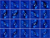 |
Fig. 1. Residual light distributions in 20 r-band sub-frames. These sub-frames are extracted from frames taken with the IO:O camera of the LT in good seeing conditions, and they show well-structured extra-stellar residues in the region occupied by the lensing galaxy. |
2.3. Final photometric model
In general, frames were taken under seeing conditions worse than ∼1″, so we blurred the numerical component of the galaxy for each observed frame to account for its PSF. We used a circular Gaussian with a full width at half maximum FWHM = (FWHMobs2 − FWHMbest2)1/2 to blur the numerical component, which is sufficient for our purposes because the numerical component is only a few percent of the analytical component. To obtain the quasar fluxes, the final photometric model consisted of four key elements: four empirical PSFs (quasar images), DV and exponential brightness distributions convolved with the empirical PSF, a numerical galaxy component convolved with the corresponding circular Gaussian function, and a constant background term. After estimating a calibration factor (flux of a reference star), this more detailed model has five free parameters: the sky background level and the four quasar fluxes. We applied it to square sub-frames with 256 pixels on a side. These 256 × 256 pixel sub-frames are much larger than those with 32 pixels on a side used in previous work (see the central green square in the left panel of Figure 2), leading to robust background estimates.
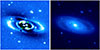 |
Fig. 2. Lensing galaxy model from the LT IO:O r-band best frames. Left: Numerical component in a square sub-frame of 256 pixels on a side. A 32 × 32 pixel green square is shown for comparison. Right: Sum of the analytical and numerical components. |
To demonstrate the performance of the new photometric approach (using a galaxy model incorporating DV, exponential disc, and numerical components in 256 × 256 pixel sub-frames) in the crowded region occupied by the quasar images, we focused on the R-band MT frames available for reanalysis and carried out a goodness-of-fit test. Figure 3 shows the new reduced chi-square (χnew2) of the central 32 × 32 pixel square shown in green in the left panel of Figure 2. These χnew2 values for 445 observing nights over 2006−2019 are distributed around a mean of 1.2 with a standard deviation of 0.3. For comparison, Figure 3 also includes the χold2 values from our previous photometric approach (using a DV galaxy model in 32 × 32 pixel sub-frames; Goicoechea et al. 2020), which are higher and show greater dispersion (mean of 2.1 and standard deviation of 1), indicating a larger discrepancy between the observed and modelled light distributions.
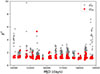 |
Fig. 3. Values of χ2 in the central 32 × 32 pixel square containing the four quasar images when modelling MT R-band frames. The red squares correspond to the new photometric scheme and the grey circles correspond to our previous photometric method. |
3. Light curves
The extended light curves of QSO 2237+0305 include data obtained with three telescopes in six optical bands. Table 1 shows the number of observing epochs (nights) for each band and telescope. This table also includes the monitoring periods. The previous number of data points (numbers within brackets in Table 1; Goicoechea et al. 2020) is ∼40% of the current one, so we increased the database by a factor of ∼2.4. We did not reprocess the B-band exposures taken with the LT with the new photometric scheme (see Sect. 2). These exposures were so short that they yielded noisy frames that prevented an accurate estimate of the numerical galaxy model. We processed these frames with a simpler photometric method using only a DV surface brightness for the lensing galaxy. The MT frames from the period 1995−2005 and some MT frames in 2006−2008 were not available for reanalysis.
Number of observing epochs (nights) for each band and telescope.
3.1. Monitoring with LT in the BgVr bands
Monitoring in the gr bands used two different CCD cameras: RATCam ( /pixel) over 2006−2009 and IO:O (
 /pixel) over 2013−2024. Each IO:O observing night, we took one 300 s (180 s) exposure in the g (r) band. We present updated GLENDAMA light curves for the g and r bands in the top and bottom panels of Figure 4, respectively, and in Tables C.1 (g band) and C.2 (r band). These long photometric tables are available at the CDS in a standard format containing epochs, magnitudes, and magnitude errors. The new photometric method mainly produces small increases in brightness in the light curves of the C and D images compared to our earlier light curves, with larger increases when the image is fainter. In addition to these magnitude offsets, which are probably related to adequate subtraction of the sky background, the scatter is reduced, presumably due to our improved modelling of the observed light distributions. The top and bottom panels of Figure 4 also show that the four images present roughly similar variations over the last five years. We also note a significant extrinsic variation in image D in 2019.
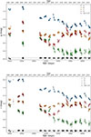 |
Fig. 4. Updated GLENDAMA light curves of QSO 2237+0305. We added new data from monitoring with the LT over 2020−2024. Top: g-band magnitudes. Bottom: r-band magnitudes. |
In addition, we analysed the LT IO:O frames in the BV bands. This programme typically consisted of 4 × 20 s B-band exposures and 4 × 25 s V-band exposures every observing night. The signal-to-noise ratio of the short exposures in the B band is lower than that of the gr bands, but it allowed us to extend the B-band monitoring period by three additional years.
3.2. Monitoring with MT in the BVRI bands
We obtained MT frames from 2006−2019 with two CCD cameras: SNUCAM ( /pixel) and FLI MicroLine (
 /pixel). The average exposure time per night was relatively long (1290 s), and the average seeing per night was reasonably good (
 ). The R-band light curve is the best sampled, with lower sampling rates for the VI bands and very poor sampling for the B band (see Figures 5 and 6). After reprocessing all available MT frames, we found that the new refined photometry for 2006−2008 closely follows previously published MT brightness records for that period (Dudinov et al. 2010). We found only small constant magnitude offsets between the two. Hence, although the magnitudes of Dudinov et al. (2010) from 2001 to 2008 are based on a photometric method different from ours, we used their light curves for the period 2001−2008 after correcting for the magnitude offsets. We then extended the MT records by six more years (1995−2000) using magnitudes from the same group obtained through photometric approaches consistent with our refined photometry (Vakulik et al. 2004). This dataset includes only one night in 1995 – regular monitoring only started in 1997.
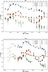 |
Fig. 5. Updated B-band (top) and V-band (bottom) light curves. |
3.3. Monitoring with ST in the BVRI bands
The ST BVRI observations performed with the ANDICAM camera ( /pixel; DePoy et al. 2003) over the period 2004−2017 typically consist of three 300 s exposures per night in each filter, with basic instrumental reductions applied to all ST frames (i.e. bias subtraction, trimming of the overscan regions, flat-fielding, and cosmic-ray cleaning). We processed the frames with our new photometric method to extract the quasar magnitudes. To obtain the final combined VRI light curves (see the three corresponding panels of Figures 5 and 6), we considered the MT magnitudes as a reference and corrected the LT and ST data for small constant magnitude offsets. However, the number of MT B-band epochs is small (see Table 1), so we used the ST B-band magnitudes as a reference to build the combined light curves in that optical band and corrected the LT and MT data with small magnitude offsets (see the top panel of Figure 5). These data are available in Tables C.3 (B band), C.4 (V band), C.5 (R band), and C.6 (I band) at the CDS, with the last column indicating the facility.
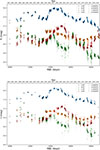 |
Fig. 6. Updated R-band (top) and I-band (bottom) light curves. |
3.4. Error estimation and short-term variability
For each band and telescope, we estimated typical magnitude errors of the four quasar images and a control star. We used the PSF1 star in Fig. 1 of Eigenbrod et al. (2008a) (it is the so-called β star in Fig. 1 of Corrigan et al. 1991) as a control object with a constant true magnitude in each optical band. For a given band, the true magnitude of PSF1 is close to the average magnitude of a quasar image, so the PSF1 star is well-suited for checking the reliability of typical magnitude errors of the quasar in that band. For example, if we focus on MT R-band data, the true magnitude of PSF1 (∼18 mag) is similar to the average R-band magnitude of B. Thus, for each quasar image and the PSF1 star, we calculated the standard deviation between MT R-band magnitudes with time separations ≤2.5 d, and then divided it by the square root of two to obtain the typical error. As expected, the typical errors of image B and the control star have similar values and amount to ∼2%, while we achieve ∼3% photometry from MT R-band observations of image C, which show episodes with a brightness ∼1 mag greater than that of the control star.
For each quasar image, we also estimated uncertainties at every epoch by weighting its typical error by the ⟨S/N⟩/S/N ratio (e.g. Howell 2006), where S/N is the signal-to-noise ratio and ⟨S/N⟩ is the average S/N. It is worth noting that these individual photometric uncertainties are distributed around typical errors, which significantly exceed theoretical ones based on expected noise sources in image formation and excluding dominant systematic effects.
We show the short-term multi-band variability over three well-sampled time periods spanning one or two years in Figures A.1, A.2, and A.3 in Appendix A. These zoomed-in multi-band light curves clearly display intra-year and year-to-year chromatic variations exceeding the observational noise. For example, in 2013 (see Figure A.1), we compare the optically quiescent image B with the optically active image D. On a timescale of ∼100 d, the brightness of D decreases by ∼0.5 mag in the Bg blue bands, but only by ∼0.3 mag in the R band. Additionally, in 2015−2016 (see Figure A.2), the brightness of C drops by ∼1 mag over ∼1 yr in the g band. However, the brightness gradient in image C is appreciably less pronounced in the I band.
4. Microlensing variability
4.1. Difference light curves
Since the time delays between the quasar images in QSO 2237+0305 are less than one day (e.g. Dai et al. 2003; Vakulik et al. 2006; Berdina & Tsvetkova 2017), the observed microlensing signals are simply differences between light curves, usually using image pairs (e.g. Vernardos et al. 2024). Here, we used four non-standard DLCs in each optical band: A − (B + C + D)/3, B − (A + C + D)/3, C − (A + B + D)/3, and D − (A + B + C)/3, which we denote as DLC A–D and which we show in Figure 7 (see also Appendix B). These DLCs fully remove the intrinsic variability of the quasar and minimise the microlensing contribution from the three subtracted curves to the signal in the first.
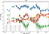 |
Fig. 7. Difference light curves in the BgVrRI bands. Squares with black borders indicate the microlensing signals in the V band. Details of the DLCs in five well-sampled observing seasons are shown in Appendix B. |
In the absence of microlensing effects produced by stars, the DLCs would be constant but band-dependent due to extinction differences. The DLCs in Figure 7 clearly show strong microlensing-induced variability that also depends on the band, since microlensing signal amplitudes are related to the source size, which depends on the wavelength (e.g. Schneider et al. 1992; Vernardos et al. 2024). Isolated high-magnification events appear, for example, in DLC A in 2016, DLC B in 2005, DLC C in 1999, and DLC D in 2019. Moreover, DLC C shows evidence of a double caustic crossing event covering the period 2011−2016, first detected by Goicoechea et al. (2020) and currently under detailed numerical simulation analysis.
As a first approach to quantifying microlensing, we computed the root-mean-square dispersion σ for each image and band over well-sampled time periods (2004−2019 for BVRI and 2013−2024 for gr; see Figures 4, 5, and 6). We list these values in Table 2 and show them in Figure 8. Standard error propagation yields uncertainties of a few percent in the σ values, which we do not include in Table 2, but consider in Sect. 4.2. Figure 8 shows that images C and D have significantly higher microlensing variability than images A and B, consistent with theoretical predictions based on the convergence, shear, and compact-object mass fraction (stars) at the image positions (e.g. Seitz et al. 1994; Lewis & Irwin 1996). Additionally, microlensing variability is lower at longer wavelengths, as expected for a source size-wavelength relationship Rs ∝ λα with α > 0. Guerras et al. (2020) show that comparing the measured values of σ with those from simulated DLCs may provide relevant information on the X-ray sources, based on X-ray observations of a sample of quadruply-imaged quasars. Thus, we explored a similar approach using our optical DLCs.
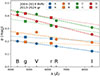 |
Fig. 8. Root mean square microlensing variability for all images as a function of wavelength. We show linear fits for each of the two gap-free time periods: 2004−2019 (dashed lines) and 2013−2024 (dotted lines). |
Standard deviations of the DLCs (in mag).
For a more quantitative analysis, we created magnification maps for the quasar images using the convergences, shear strengths, and microlens mass fractions from Table 1 of Guerras et al. (2020). We randomly selected stars from a mass function dN/dM ∝ M−1.3 with a maximum-to-minimum mass ratio of 50 (Gould 2000). We generated source-plane magnification maps for a point-like source (one-pixel size) using the Poisson and inverse polygon (PIP) method4 (Shalyapin et al. 2021). This publicly available software makes map generation quick and simple. We convolved the maps with Gaussian kernels exp(−r2/2R2), where Rs = 1.177 R is the half-light radius of the source in units of the Einstein radius of a star with mean mass ⟨M⟩ (RE).
To account for random motions of stars, we created dynamic maps (Wambsganss & Kundić 1995; Poindexter & Kochanek 2010a,b), which we call magnification ‘cubes’. We created these animated sequences of static magnification patterns assuming a typical ratio of 2.5 between the effective speed of the source in the lens plane vt (its probability distribution has a peak around 400 km s−1; see Fig. 5 of Poindexter & Kochanek 2010a) and the stellar velocity dispersion of the lensing galaxy σ* ∼ 160 − 170 km s−1 (Trott et al. 2010; van de Ven et al. 2010). Rather than using a Gaussian distribution of stellar velocities, we treated the stellar motions in the lens plane as a distribution of velocities with the same modulus σ* and arbitrary directions.
We considered magnification maps of 25 RE on a side at 2500 × 2500 pixel resolution (i.e. 100 pix/RE) and verified that larger maps produce similar results. For each optical band, we produced simulated light curves for the four quasar images with the same time sampling as the observations. We selected random starting points on each first image map (first map of the image cube) and used the same source trajectory for all images. Each trajectory has a length L and a direction depending on the shear orientation of the image (Witt & Mao 1994; Poindexter & Kochanek 2010a). Figure 9 shows an example with L = 5 RE for the four images. We used the PIP software and a step of 0.2 RE for the source displacement, which implies that the stars were displaced by 0.08 RE at each simulation step. This source-to-stars displacement ratio of 2.5 coincides with the vt/σ* ratio.
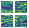 |
Fig. 9. (Movie online) Animated sequence of magnification maps corresponding to 25 simulation steps of 0.2 RE each. The white line is the source trajectory across the sky, which is rotated in the B, C, and D magnification cubes with respect to cube A because of misalignments between the coordinate systems. For each quasar image, the shear direction coincides with the x axis in the corresponding magnification map, and the four shear directions form different angles with respect to celestial north. |
For each source trajectory, we obtained four simulated light curves, which allowed us to build synthetic DLCs. There are constant offsets between the observed and synthetic DLCs because our simulations ignore dust extinction effects; however, these do not affect the DLC dispersions. The amount of microlensing variability of a quasar image (standard deviation of its DLC) is related to the source radius, Rs (the larger the source, the smaller the variations), and the trajectory length, L (longer trajectories have larger variations). The source trajectory angle, θ (measured east of north), also plays a role (e.g. Wambsganss et al. 1990). For each optical band and quasar image, we searched for (Rs, L, θ) values yielding a simulated standard deviation σsim (average for a representative set of starting points) equal to the observed one σobs.
4.2. Accretion disc structure
Figure 10 shows the g-band data (see the σobs values in the third row of Table 2) used to estimate the source size. For the Einstein Cross, several previous studies indicated that Rs at optical wavelengths is appreciably smaller than RE (e.g. Kochanek 2004; Anguita et al. 2008; Poindexter & Kochanek 2010a,b). Hence, we considered 100 uniformly distributed Rs values, ranging from 0.01 RE to RE. We also tested 25 uniformly distributed L values between 0.2 and 5 RE. We used four source trajectory angles (θ = 0, 30, 60, and 90°). For every possible combination of Rs, L, and θ, we generated 1000 source trajectories, built the corresponding synthetic DLCs, calculated their standard deviations, and derived σsim for each image by averaging the 1000 individual results. Thus, for each image, setting σsim = σobs for a given value of θ, we obtain a set of pairs (Rs, L) consistent with the observations. Figure 10 shows the 16 resulting Rs − L curves (four images × four source trajectory directions).
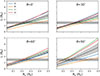 |
Fig. 10. Rs − L curves consistent with the standard deviations of the observed g-band DLCs. We consider four trajectory angles measured east of north (θ = 0, 30, 60, and 90°). The inclined dashed black lines and the grey regions around them describe the average Rs − L curves and their standard error bands, while the horizontal dashed black line and the horizontal grey strip represent an estimate of the trajectory length. |
Regarding the direction of motion of the source, the four Rs − L curves for an angle of 30° east of north are slightly closer to each other than those for the 60° angle, but clearly closer together than for the other two values of θ. Additionally, Fig. 4 of Poindexter & Kochanek (2010a) shows the θ probability peaks in the 30−60° interval. We constructed an average curve and calculated its standard error band (dashed black line and grey region around it) from the four coloured lines in the top right panel of Figure 10 (θ = 30°). We also estimated the trajectory length of the g-band source. We adopted a concordance flat cosmology and a standard mean mass ⟨M⟩ = 0.3 M⊙, yielding RE = 1017 cm (e.g. Poindexter & Kochanek 2010a,b). As the g-band data span about 11.5 yr, L ∼ 1.5 RE for a typical vt of ∼400 km s−1 (see above). We assumed that the actual vt is within a 15% interval around its typical value, that is, the true transverse speed can be up to 15% lower or higher than the typical value (grey region around the horizontal dashed black line). This speed interval (400 ± 60 km s−1) agrees with the speed distribution peak in Fig. 5 of Poindexter & Kochanek (2010a). The intersection between the two grey regions in the top right panel of Figure 10 yields Rs = (0.25 ± 0.07) RE for the half-light radius of the g-band source. An analysis of the results in the bottom left panel of Figure 10 (θ = 60°) yields a measurement of Rs in good agreement with that for θ = 30°.
In our g-band data analysis, we considered central values of σobs (see Table 2). We also accounted for small uncertainties of a few percent. Thus, for each value of θ, we obtained a strip around each Rs − L curve by searching for pairs (Rs, L) producing σsim values within the measured interval for σobs. The four strips (one per quasar image) are much thinner than the separation between them, so they do not affect the estimation of Rs from the central σobs values.
A caveat to our approach is that it neglects pairs (Rs, L) corresponding to σsim values outside the measured intervals for σobs. Although we expect a small dispersion of standard deviations for a representative set of large simulated trajectories, the dispersion is higher for trajectories of a few Einstein radii. Therefore, values of σsim other than the central values of σobs could give rise to a relatively wide probability band for each image, with probability peaks along the central Rs − L curves. Here we assume that these probability peaks for each direction in Figure 10 provide reliable uncertainties on the estimation of Rs, although they might be slightly underestimated.
We also note that L/RE ∝ vt/⟨M⟩1/2 for a given observation period. Hence, while L/RE depends on ⟨M⟩1/2 and the mean mass is not expected to deviate much from 0.3 M⊙, the actual transverse speed could lie outside the interval considered here, so the source-size measurement would be biased. However, although we cannot rule out values of vt close to 200 or 700 km s−1, their probability is appreciably lower than that of the peak of the speed distribution. The relative probabilities of θ = 0 and 90° are also clearly lower than those of 30−60°. A detailed interpretation of the observed microlensing signals will be presented in a separate study.
With our BVRI long-term optical monitoring data, which cover the optical spectrum almost uniformly and span the same well-sampled period (2004−2019), we also constrain the wavelength dependence of the accretion disc size, Rs ∝ λα. We followed the procedure described above for these BVRI bands. For each optical band, we derived 16 values of Rs from the intersections of all Rs − L curves (corresponding to the four source trajectory angles for each quasar image; see Figure 10) and a horizontal line at the typical trajectory length of 2 RE (BVRI data span 15.5 yr rather than 11.5 yr). Figure 11 shows these results, where each colour corresponds to an image, and each panel shows results for a trajectory angle.
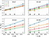 |
Fig. 11. Source radius versus wavelength for four source trajectory angles and the four quasar images. The results for images A, B, C, and D are shown in blue, orange, green, and red, respectively. |
Considering all images, we obtain quasi-linear Rs − λ relations with α = 0.92 ± 0.02 for θ = 30° and α = 0.96 ± 0.07 for θ = 60°. The overall slope is α = 0.97 ± 0.15 (for all angles and images). A strength of this analysis is the stability of the slopes against changes in the adopted trajectory length (depending on vt). Although changes in the height of the horizontal line describing the adopted value for L (deviations from the typical length; see Figure 10) produce a systematic increase or decrease of all values of Rs, the slopes remain essentially unchanged.
5. Conclusions
The GLENDAMA project has been monitoring ten gravitationally lensed quasars for the last 20 years with the LT at the Roque de los Muchachos Observatory (La Palma, Spain; Gil-Merino et al. 2018). We present a new photometric method to extract magnitudes of the four optical images of the quadruply lensed quasar QSO 2237+0305, the Einstein Cross, which is a target of the GLENDAMA sample. We applied the new photometric scheme to LT observations and other monitoring campaigns at the Maidanak Astronomical Observatory (Uzbekistan) and the Cerro Tololo Inter-American Observatory (Chile). In total, the baseline monitoring time of the Einstein Cross extends to 30 years, and the associated light curves describe the variability in the BgVrRI optical bands. This represents a substantial effort to treat and combine data from a wide variety of instruments and observing conditions.
As a result, we provide DLCs within the new global dataset (Figure 7), where the extrinsic variability due to microlensing effects at the position of the quasar images can be analysed with high accuracy. Microlensing signals exhibit sharp variations that depend on wavelength, making them promising features for resolving the controversy over the structure of the quasar accretion disc (e.g. Eigenbrod et al. 2008b; Muñoz et al. 2016; Goicoechea et al. 2020). Although long-term optical monitoring is usually conducted in a single band-pass filter and thus cannot constrain the accretion disc structure, the source radius-wavelength relationship Rs ∝ λα can be probed with our long-term follow-up of the variability of QSO 2237+0305 from the blue to the near-infrared part of its spectrum. A detailed analysis of the new DLCs from microlensing simulations based on large, high-resolution magnification maps will be presented in a forthcoming paper.
However, we performed a preliminary study of the accretion disc structure solely using the root mean square DLC dispersions over well-sampled time periods (Table 2). We compared these wavelength-dependent standard deviations for each quasar image to those from simulated DLCs for Gaussian source trajectories across dynamic magnification maps. Our simulated DLCs account for stellar random motions and are sampled in the same way as the observed ones. Adopting a mean microlens mass ⟨M⟩ = 0.3 M⊙ and reasonable constraints on the effective velocity of the source in the lens plane (400 ± 60 km s−1 with a position angle within the interval 30−60°; Poindexter & Kochanek 2010a), we measure the half-light radius Rs of the g-band source (Figure 10) and derive a power-law index of α ∼ 1 (Figure 11) rather than the value predicted by the geometrically-thin, optically-thick standard disc theory (α = 4/3; Shakura & Sunyaev 1973). Microlensing analyses of other lensed quasars also found slopes shallower than the standard one (e.g. Blackburne et al. 2011), whereas Cornachione & Morgan (2020) generally find slopes steeper than the standard model from quasar variability studies (temperature profiles shallower than the standard one).
For the g-band source, we find Rs to be in the range of 7 − 12 lt-day, in very good agreement with the measurements of Muñoz et al. (2016) at ∼4700 Å for Gaussian, hybrid, and standard-disc sources (scaled to ⟨M⟩ = 0.3 M⊙), but somewhat larger than the upper limit of ∼6 lt-day on the g-band half-light radius from the analysis of the high-magnification event in image C in 1999 (see Sect. 2), using a Gaussian source model without any prior on the velocity of the lens galaxy (Anguita et al. 2008). In addition, our results indicate a source size that grows with wavelength with a power-law index (slope) of α = 0.94 ± 0.05 (averaging the central values and errors for position angles of 30 and 60°). This slope is consistent with those reported by Eigenbrod et al. (2008b) and Muñoz et al. (2016), but shallower than the standard disc model at ∼8σ significance. Even assuming a possible underestimation of the error in α by a factor of two or three, a standard accretion disc faces serious difficulties as the sole source of UV-optical continuum radiation in QSO 2237+0305. Gaskell (2008) suggested a model with a much more inconsistent slope (α = 1.75) than the standard value, while α = 8/7 if the disc is powered by the spin of the central black hole (Agol & Krolik 2000). Although a non-standard accretion disc model can reproduce the observations, optical passband fluxes originate in the central accretion disc and the broad emission-line region (e.g. Korista & Goad 2001), so the measured relationship between source size and wavelength could be considerably flattened if the contribution of the extended region is substantial (e.g. Fian et al. 2023).
This long-term multi-band photometric monitoring opens a window for crucial tests of the quasar structure and demonstrates that microlensing can reveal possible deviations from a standard accretion disc scenario. Further analysis of other lensed quasars of the GLENDAMA sample, as well as the implementation of larger, high-resolution magnification map cubes for the full light curves, would provide stronger constraints for comparison with results obtained in this and other works.
Data availability
Tables C.1–C.6 are available available at the CDS via https://cdsarc.cds.unistra.fr/viz-bin/cat/J/A+A/710/A70. Movie associated with Fig. 9 is available at https://www.aanda.org
Acknowledgments
We thank Christopher Kochanek (CK) for his comments and suggestions, which have helped us to significantly improve an initial version of the manuscript. The Liverpool Telescope (LT) is operated on the island of La Palma by Liverpool John Moores University in the Spanish Observatorio del Roque de los Muchachos of the Instituto de Astrofísica de Canarias with financial support from the UK Science and Technology Facilities Council. We thank the staff of the LT for a kind interaction. The 1.5 m Maidanak Telescope is a facility of the Ulugh Beg Astronomical Institute of the Uzbekistan Academy of Sciences, which is operated on the Maidanak Astronomical Observatory (MAO) by a consortium of various international institutions. We thank Boris Artamonov, Otabek Burkhonov, Talat Akhunov, Ildar Asfandiyarov, Vasily Bruevich, and Shuhrat Ehgamberdiev, who organized and carried out the observations of the Einstein Cross at the MAO. The 1.3 m SMARTS Telescope is operated on the Cerro Tololo Inter-American Observatory by the SMARTS Consortium, and the Einstein Cross monitoring program was led by CK. VNS acknowledges the Universidad de Cantabria (UC) and the Spanish Agencia Estatal de Investigacion (AEI) for financial support for a long stay at the UC in the period 2022–2024. AEG acknowledges support from project ANID Fondecyt Postdoctorado with grant number 3230554. This research was supported by the grant PID2020-118687GB-C31, financed by the Spanish Ministerio de Ciencia e Innovación through MCIN/AEI/10.13039/501100011033. This research has also been supported by UC funds and the grant PID2020-118990GB-I00 funded by MCIN/AEI/10.13039/501100011033.
References
- Agol, E., & Krolik, J. 1999, ApJ, 524, 49 [Google Scholar]
- Agol, E., & Krolik, J. H. 2000, ApJ, 528, 161 [NASA ADS] [CrossRef] [Google Scholar]
- Alcalde, D., Mediavilla, E., Moreau, O., et al. 2002, ApJ, 572, 729 [Google Scholar]
- Anguita, T., Schmidt, R. W., Turner, E. L., et al. 2008, A&A, 480, 327 [NASA ADS] [CrossRef] [EDP Sciences] [Google Scholar]
- Berdina, L. A., & Tsvetkova, V. S. 2017, Adv. Astron. Space Phys., 7, 12 [Google Scholar]
- Best, H., Fagin, J., Vernardos, G., & O’Dowd, M. 2024, MNRAS, 531, 1095 [Google Scholar]
- Blackburne, J. A., Pooley, D., Rappaport, S., & Schechter, P. L. 2011, ApJ, 729, 34 [Google Scholar]
- Cornachione, M. A., & Morgan, C. W. 2020, ApJ, 895, 93 [Google Scholar]
- Corrigan, R. T., Irwin, M. J., Arnaud, J., et al. 1991, AJ, 102, 34 [NASA ADS] [CrossRef] [Google Scholar]
- Dai, X., Chartas, G., Agol, E., Bautz, M. W., & Garmire, G. P. 2003, ApJ, 589, 100 [NASA ADS] [CrossRef] [Google Scholar]
- De Vaucouleurs, G. 1948, Ann. Astrophys., 11, 247 [Google Scholar]
- DePoy, D. L., Atwood, B., Belville, S. R., et al. 2003, Proc. SPIE, 4841, 827 [NASA ADS] [CrossRef] [Google Scholar]
- Dudinov, V. N., Smirnov, G. V., Vakulik, V. G., Sergeev, A. V., & Kochetov, A. E. 2010, Radio Phys. Radio Astron., 15, 387 [NASA ADS] [Google Scholar]
- Eigenbrod, A., Courbin, F., Sluse, D., Meylan, G., & Agol, E. 2008a, A&A, 480, 647 [NASA ADS] [CrossRef] [EDP Sciences] [Google Scholar]
- Eigenbrod, A., Courbin, F., Meylan, G., et al. 2008b, A&A, 490, 933 [NASA ADS] [CrossRef] [EDP Sciences] [Google Scholar]
- Fian, C., Chelouche, D., & Kaspi, S. 2023, A&A, 677, A94 [NASA ADS] [CrossRef] [EDP Sciences] [Google Scholar]
- Gaskell, C. M. 2008, Rev. Mex. Astron. Astrofis. Conf. Ser., 32, 1 [NASA ADS] [Google Scholar]
- Gil-Merino, R., Goicoechea, L. J., Shalyapin, V. N., & Oscoz, A. 2018, A&A, 616, A118 [NASA ADS] [CrossRef] [EDP Sciences] [Google Scholar]
- Goicoechea, L. J., Artamonov, B. P., Shalyapin, V. N., et al. 2020, A&A, 637, A89 [NASA ADS] [CrossRef] [EDP Sciences] [Google Scholar]
- Gould, A. 2000, ApJ, 535, 928 [Google Scholar]
- Guerras, E., Dai, X., & Mediavilla, E. 2020, ApJ, 896, 111 [NASA ADS] [CrossRef] [Google Scholar]
- Howell, S. B. 2006, Handbook of CCD Astronomy (Cambridge: Cambridge University Press) [Google Scholar]
- Huchra, J., Gorenstein, M., Kent, S., et al. 1985, AJ, 90, 691 [NASA ADS] [CrossRef] [Google Scholar]
- Irwin, M. J., Webster, R. L., Hewitt, P. C., Corrigan, R. T., & Jedrzejewski, R. I. 1989, AJ, 98, 1989 [NASA ADS] [CrossRef] [Google Scholar]
- Isla, D., Goicoechea, L. J., Esteban-Gutiérrez, A., et al. 2025, A&A, 702, A172 [NASA ADS] [CrossRef] [EDP Sciences] [Google Scholar]
- Kochanek, C. S. 2004, ApJ, 605, 58 [Google Scholar]
- Korista, K. T., & Goad, M. R. 2001, ApJ, 553, 695 [Google Scholar]
- Lewis, G. F., & Irwin, M. J. 1996, MNRAS, 283, 225 [NASA ADS] [Google Scholar]
- McLeod, B. A., Bernstein, G. M., Rieke, M. J., & Weedman, D. W. 1998, AJ, 115, 1377 [NASA ADS] [CrossRef] [Google Scholar]
- Muñoz, J. A., Vives-Arias, H., Mosquera, A. M., et al. 2016, ApJ, 817, 155 [Google Scholar]
- Østensen, R., Refsdal, S., Stabell, R., et al. 1996, A&A, 309, 59 [NASA ADS] [Google Scholar]
- Poindexter, S., & Kochanek, C. S. 2010a, ApJ, 712, 658 [NASA ADS] [CrossRef] [Google Scholar]
- Poindexter, S., & Kochanek, C. S. 2010b, ApJ, 712, 668 [NASA ADS] [CrossRef] [Google Scholar]
- Schneider, P., Ehlers, J., & Falco, E. E. 1992, Gravitational Lensing (Berlin: Springer) [Google Scholar]
- Seitz, C., Wambsganss, J., & Schneider, P. 1994, A&A, 288, 19 [Google Scholar]
- Shakura, N. I., & Sunyaev, R. A. 1973, A&A, 24, 337 [NASA ADS] [Google Scholar]
- Shalyapin, V. N., Gil-Merino, R., & Goicoechea, L. J. 2021, A&A, 653, A121 [NASA ADS] [CrossRef] [EDP Sciences] [Google Scholar]
- Sorgenfrei, C., Schmidt, R. W., & Wambsganss, J. 2025, A&A, 703, A250 [NASA ADS] [CrossRef] [EDP Sciences] [Google Scholar]
- Sparke, L. S., & Gallagher, J. S., III 2007, Galaxies in the Universe: An Introduction (Cambridge: Cambridge University Press) [Google Scholar]
- Steele, I. A., Smith, R. J., Rees, P. C., et al. 2004, Proc. SPIE, 5489, 679 [NASA ADS] [CrossRef] [Google Scholar]
- Trott, C. M., Treu, T., Koopmans, L. V. E., & Webster, R. L. 2010, MNRAS, 401, 1540 [NASA ADS] [CrossRef] [Google Scholar]
- Tuntsov, A. V., Lewis, G. F., & Walker, M. A. 2024, MNRAS, 528, 1979 [Google Scholar]
- Udalski, A., Szymański, M. K., Kubiak, M., et al. 2006, Acta Astron., 56, 293 [Google Scholar]
- Vakulik, V. G., Schild, R. E., Dudinov, V. N., et al. 2004, A&A, 420, 447 [NASA ADS] [CrossRef] [EDP Sciences] [Google Scholar]
- Vakulik, V., Schild, R., Dudinov, V., et al. 2006, A&A, 447, 905 [NASA ADS] [CrossRef] [EDP Sciences] [Google Scholar]
- van de Ven, G., Falcón-Barroso, J., McDermid, R. M., et al. 2010, ApJ, 719, 1481 [Google Scholar]
- Vernardos, G., Sluse, D., Pooley, D., et al. 2024, Space Sci. Rev., 220, 14 [NASA ADS] [CrossRef] [Google Scholar]
- Wambsganss, J., & Kundić, T. 1995, ApJ, 450, 19 [Google Scholar]
- Wambsganss, J., & Paczyński, B. 1991, AJ, 102, 864 [NASA ADS] [CrossRef] [Google Scholar]
- Wambsganss, J., Paczyński, B., & Katz, N. 1990, ApJ, 352, 407 [NASA ADS] [CrossRef] [Google Scholar]
- Witt, H. J., & Mao, S. 1994, ApJ, 429, 66 [Google Scholar]
- Woźniak, P. R., Udalski, A., Szymański, M., et al. 2000, ApJ, 540, L65 [CrossRef] [Google Scholar]
- Yonehara, A., Mineshige, S., Manmoto, T., et al. 1998, ApJ, 501, L41 [Google Scholar]
It is commonly assumed that optical passband fluxes originate in the central accretion disc.
CASTLES database of QSO 2237+0305 at https://lweb.cfa.harvard.edu/castles/Individual/Q2237.html, updated on 21 July 2021 (C. S. Kochanek, E. E. Falco, C. Impey, J. Lehar, B. McLeod, H.-W. Rix).
Appendix A: Zoomed-in multi-band light curves
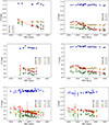 |
Fig. A.1. Multi-band light curves in 2013. Regarding the variability of images B and D, we show dashed lines as a guide to the eye. |
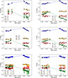 |
Fig. A.2. Multi-band light curves in 2015−2016. We include dashed lines as a guide to the eye. |
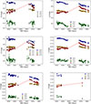 |
Fig. A.3. Multi-band light curves in 2018−2019. We include dashed lines as a guide to the eye. |
Appendix B: Zoomed-in multi-band DLCs
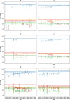 |
Fig. B.1. Multi-band DLCs in 2013. The horizontal dashed lines and the associated horizontal strips represent the average error bars for the four images in the six bands. |
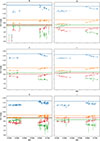 |
Fig. B.2. Multi-band DLCs in 2015−2016. The horizontal dashed lines and the associated horizontal strips represent the average error bars for the four images in the six bands. |
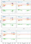 |
Fig. B.3. Multi-band DLCs in 2018−2019. The horizontal dashed lines and the associated horizontal strips represent the average error bars for the four images in the six bands. |
All Tables
All Figures
|
Fig. 1. Residual light distributions in 20 r-band sub-frames. These sub-frames are extracted from frames taken with the IO:O camera of the LT in good seeing conditions, and they show well-structured extra-stellar residues in the region occupied by the lensing galaxy. |
| In the text | |
|
Fig. 2. Lensing galaxy model from the LT IO:O r-band best frames. Left: Numerical component in a square sub-frame of 256 pixels on a side. A 32 × 32 pixel green square is shown for comparison. Right: Sum of the analytical and numerical components. |
| In the text | |
|
Fig. 3. Values of χ2 in the central 32 × 32 pixel square containing the four quasar images when modelling MT R-band frames. The red squares correspond to the new photometric scheme and the grey circles correspond to our previous photometric method. |
| In the text | |
|
Fig. 4. Updated GLENDAMA light curves of QSO 2237+0305. We added new data from monitoring with the LT over 2020−2024. Top: g-band magnitudes. Bottom: r-band magnitudes. |
| In the text | |
|
Fig. 5. Updated B-band (top) and V-band (bottom) light curves. |
| In the text | |
|
Fig. 6. Updated R-band (top) and I-band (bottom) light curves. |
| In the text | |
|
Fig. 7. Difference light curves in the BgVrRI bands. Squares with black borders indicate the microlensing signals in the V band. Details of the DLCs in five well-sampled observing seasons are shown in Appendix B. |
| In the text | |
|
Fig. 8. Root mean square microlensing variability for all images as a function of wavelength. We show linear fits for each of the two gap-free time periods: 2004−2019 (dashed lines) and 2013−2024 (dotted lines). |
| In the text | |
|
Fig. 9. (Movie online) Animated sequence of magnification maps corresponding to 25 simulation steps of 0.2 RE each. The white line is the source trajectory across the sky, which is rotated in the B, C, and D magnification cubes with respect to cube A because of misalignments between the coordinate systems. For each quasar image, the shear direction coincides with the x axis in the corresponding magnification map, and the four shear directions form different angles with respect to celestial north. |
| In the text | |
|
Fig. 10. Rs − L curves consistent with the standard deviations of the observed g-band DLCs. We consider four trajectory angles measured east of north (θ = 0, 30, 60, and 90°). The inclined dashed black lines and the grey regions around them describe the average Rs − L curves and their standard error bands, while the horizontal dashed black line and the horizontal grey strip represent an estimate of the trajectory length. |
| In the text | |
|
Fig. 11. Source radius versus wavelength for four source trajectory angles and the four quasar images. The results for images A, B, C, and D are shown in blue, orange, green, and red, respectively. |
| In the text | |
|
Fig. A.1. Multi-band light curves in 2013. Regarding the variability of images B and D, we show dashed lines as a guide to the eye. |
| In the text | |
|
Fig. A.2. Multi-band light curves in 2015−2016. We include dashed lines as a guide to the eye. |
| In the text | |
|
Fig. A.3. Multi-band light curves in 2018−2019. We include dashed lines as a guide to the eye. |
| In the text | |
|
Fig. B.1. Multi-band DLCs in 2013. The horizontal dashed lines and the associated horizontal strips represent the average error bars for the four images in the six bands. |
| In the text | |
|
Fig. B.2. Multi-band DLCs in 2015−2016. The horizontal dashed lines and the associated horizontal strips represent the average error bars for the four images in the six bands. |
| In the text | |
|
Fig. B.3. Multi-band DLCs in 2018−2019. The horizontal dashed lines and the associated horizontal strips represent the average error bars for the four images in the six bands. |
| In the text | |
Current usage metrics show cumulative count of Article Views (full-text article views including HTML views, PDF and ePub downloads, according to the available data) and Abstracts Views on Vision4Press platform.
Data correspond to usage on the plateform after 2015. The current usage metrics is available 48-96 hours after online publication and is updated daily on week days.
Initial download of the metrics may take a while.