| Issue |
A&A
Volume 710, June 2026
|
|
|---|---|---|
| Article Number | A85 | |
| Number of page(s) | 10 | |
| Section | Planets, planetary systems, and small bodies | |
| DOI | https://doi.org/10.1051/0004-6361/202659179 | |
| Published online | 02 June 2026 | |
Atmospheric characterisation of HIP 67522 b with VLT/CRIRES+
VLT/CRIRES+ suggests a heavier planet and hints at deuterium fractionation
1
Institut de Recherche en Astrophysique et Planétologie, Université de Toulouse,
CNRS UMR 5277, 14 avenue Edouard Belin,
31400
Toulouse,
France
2
Department of Physics, University of Oxford,
Oxford
OX1 3RH,
UK
3
LIRA, Observatoire de Paris, Université PSL, CNRS, Sorbonne Université, Université Paris Cité,
5 place Jules Janssen,
92195
Meudon,
France
4
Laboratoire Lagrange, Observatoire de la Côte d’Azur, CNRS, Université Côte d’Azur,
Nice,
France
5
Centro de Astrobiología (CAB),
CSIC-INTA, Camino Bajo del Castillo s/n, 28692 Villanueva de la Cañada,
Madrid,
Spain
6
Center for Astrophysics | Harvard & Smithsonian,
60 Garden St,
Cambridge,
MA
02138,
USA
7
Department of Physics, University of Warwick,
Coventry
CV4 7AL,
UK
★ Corresponding author: This email address is being protected from spambots. You need JavaScript enabled to view it.
Received:
28
January
2026
Accepted:
21
April
2026
Abstract
Context. Young transiting exoplanets provide unique opportunities to probe planetary atmospheres during critical early phases of evolution when atmospheric escape and contraction are most active. HIP 67522 b, a 17 Myr old hot Jupiter with an extraordinarily low bulk density (<0.20 g cm−3), represents an ideal target for high-resolution transmission spectroscopy.
Aims. We aim to constrain the mass and characterise the atmospheric composition, thermal structure, and dynamics of HIP 67522 b using ground-based high-resolution near-infrared spectroscopy with VLT/CRIRES+, complementing recent JWST observations.
Methods. We obtained 92 high-resolution spectra (R ≈ 105) with VLT/CRIRES+ in the K2166 band during a transit on 30 January 2025. We applied cross-correlation techniques and Bayesian nested sampling retrievals to constrain molecular abundances, temperature structure, and atmospheric dynamics.
Results. We detected H2O at 20σ and CO at 5σ, confirming the extremely extended atmosphere of this low-mass giant. A velocity offset of −2.9 ± 0.2 km s−1 indicates day-to-night winds. The rotation velocity has been constrained to <1.8 km s−1 at 3σ, consistent with tidal locking. The retrieval analysis suggests a planetary mass of 27.7−5.5+5.9 Earth masses and statistically favours a two-temperature atmospheric structure with a discrete change at mbar pressures over an isothermal profile. This mass is twice as high as the mass estimated from JWST atmospheric observations and inconsistent at 3σ, casting doubt on the actual planetary density of the planet. No matter the choice of atmospheric model, we derived a supersolar C/O ratio that is about 1.5 times solar, along with a supersolar metallicity that might further increase if the atmosphere is cloudy, which is a degeneracy that our data alone cannot resolve. We report a tentative 2σ detection of HDO with an extreme enrichment factor of ∼1000 relative to the protosolar D/H ratio. If confirmed, this would be the first detection of deuterium in an exoplanet atmosphere and would require an intense escape rate to confirm its presence.
Key words: techniques: spectroscopic / planets and satellites: atmospheres / planets and satellites: individual: HIP 67522
© The Authors 2026
 Open Access article, published by EDP Sciences, under the terms of the Creative Commons Attribution License (https://creativecommons.org/licenses/by/4.0), which permits unrestricted use, distribution, and reproduction in any medium, provided the original work is properly cited.
This article is published in open access under the Subscribe to Open model. This email address is being protected from spambots. You need JavaScript enabled to view it. to support open access publication.
1 Introduction
Young transiting exoplanets (<100 Myr) represent crucial laboratories for understanding planetary formation as they enable the direct observation of planets still undergoing contraction, cooling, and atmospheric escape. These systems provide empirical benchmarks for theories of evolution during the critical first hundred million years of stellar evolution. Probing the atmospheres of these young planets offers a unique window into the early stages of planetary evolution, when key processes such as atmospheric escape and orbital migration are most active (Owen 2019; Baruteau et al. 2016). The atmospheric composition, temperature structure, and dynamics of young planets carry the imprint of their formation history. However, characterising young planetary atmospheres remains challenging. Only a handful of stars younger than 100 Myr are known to host transiting planets and their youth is manifested as high magnetic activity (i.e. frequent flares and starspots), further complicating the determination of planetary masses and atmospheric properties (e.g. Rackham et al. 2018). The youngest confirmed transiting systems include TIDYE-1b (∼3 Myr; Barber et al. 2024); the Jupiter-sized planet that is still embedded in its natal disk TOI-1227 b (~8 Myr; Mann et al. 2022); K2-3 3 b (∼5-10 Myr; Mann et al. 2016); AU Mic b and c (~20-24 Myr; Plavchan et al. 2020); the remarkable four-planet V1298 Tau system (∼23 Myr; David et al. 2019); and the puzzling planet HIP 67522 b (∼17 Myr; Rizzuto et al. 2020).
HIP 67522 (=HD 120411) is a 17 Myr old early G star in the Sco-Cen association located at a distance of 127 pc (Rizzuto et al. 2020). It hosts what was previously thought to be the youngest known transiting hot Jupiter because of its radius of ~10 R⊕, HIP 67522b, with an orbital period of 6.96 days (Rizzuto et al. 2020) and a second outer planet at 14.33 days (Barber et al. 2024). Subsequently, Heitzmann et al. (2021) constrained the projected obliquity of the planet to be |λ| =  . Recent JWST/NIRSpec observations have revealed that HIP 67522 b has an extraordinarily low bulk density (<0.10 g cm−3) and suggested a mass of only 13.8 ± 1.0 M⊕ (Thao et al. 2024). This extremely low density translates into an atmospheric scale height comparable to the planetary radius itself, making HIP 67522 b one of the most favourable targets for atmospheric characterisation. The JWST transmission spectrum showed strong detections of H2O and CO2 (≥7σ), with a modest detection of CO (3.5σ) and SO2 (2 σ), indicating a metal-enriched atmosphere with 3-10 × solar metallicity and a near-solar to sub-solar C/O ratio (Thao et al. 2024).
Recent photometric monitoring campaigns with TESS and CHEOPS have revealed a remarkable property characterising this system: the orbital period of HIP 67522 b exhibits significant clustering of stellar flares, with a flare rate that is approximately nine-times higher, occurring in the 20% of the orbit immediately following planetary transit (Ilin et al. 2025b). This represents a robust detection of planet-induced stellar flaring. Follow-up radio observations at 1.1-3.1 GHz with ATCA confirmed strong radio activity consistent with coronal emission of cool dwarfs, but the expected electron cyclotron maser emission (ECME) signature of magnetic star-planet interaction was not detected. Thus, upper limits of <0.7% were set on the conversion efficiency of interaction power into radio waves (Ilin et al. 2025a).
Ground-based high-resolution spectroscopy (HRS) in the near-infrared (NIR) provides a complementary approach to space-based observations, with the ability to simultaneously constrain atmospheric composition, temperature structure, and dynamics through the Doppler shifts and line broadening of molecular absorption features (Snellen et al. 2010; Brogi et al. 2016). In this paper, we present VLT/CRIRES+ high-resolution transmission spectroscopy of HIP 67522 b in the K band (centred at 2166 nm) obtained during a transit on 30 January 2025. Our observations and data reduction are presented in Sect. 2, the cross-correlation analysis and atmospheric retrievals are detailed in Sect. 3, and we discuss our results in Sect. 4.
2 Observations and data reduction
2.1 Description of the observations
We observed HIP 67522 during a transit of the exoplanet HIP 67522 b. We used the high-resolution NIR spectrograph CRIRES+ (Dorn et al. 2023) mounted at the 8-metre Unit Telescope 3 of the Very Large Telescope on the 30 January 2025 (ESO Programme 114.28HP.001, PI: Klein). Our observations started at 04:28 UT, ended at 09:18 UT and consisted of 92 consecutive spectra, each taken with a detector integration time of 180 seconds. The observations were carried out in nodding mode, meaning that the target was alternatively positioned on two distinct positions (A and B) on the slit. The nodding procedure facilitates the data reduction and the removal of sky and instrumental background.
We used CRIRES+ in the K2166 wavelength setting covering the wavelength range between 1990 and 2472 nm over six spectral orders. We note that there are wavelength gaps between the orders. Metrology was activated during the acquisition to improve the accuracy of the wavelength solution. The 0.2″ slit was set up to yield the nominal resolving power of R ≈ 105. This dataset does not suffer from the known super-resolution issue (e.g. Nortmann et al. 2025) affecting CRIRES+ spectra, for which the point spread function (PSF) tends to be smaller than the slit width. In this case, we did not use the adaptive optics (AO) system and the PSF stayed larger than the slit throughout the observations. The seeing increased drastically in the last third of the transit and decreased the signal-to-noise ratio (S/N) accordingly, despite an improving airmass (Fig. 1).
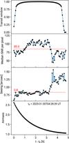 |
Fig. 1 Evolution of the transit window, the median S/N per exposure, seeing, and airmass as a function of time from the first exposure. The median S/N and median seeing for the full time-series are indicated in red on the second and third panel respectively. The UT time at the start of the first exposure t0 is indicated on the fourth panel. |
2.2 Data reduction
The data were reduced with the CRIRES+ data reduction system (DRS) cr2res, available from the ESO website1. In a first step, the raw calibrations (i.e. flat fields, darks, Fabry-Perot etalon, uranium-neon lamp) taken as part of the VLT daily calibration routine and associated to our science data were reduced using the standard calibration cascade, as described in the CRIRES+ pipeline user manual. This step yields reduced calibrations as follows: (1) normalised flat fields characterising pixel-to-pixel sensitivity variations; (2) a bad pixel mask; and (3) a so-called tracewave file containing the locations of the spectral orders on the detectors, the slit curvature, and the wavelength solution. In a second step, the reduced calibrations were applied to pairs of spectra taken in nodding positions A and B. Finally, 1D spectra were extracted with the cr2res_obs_nodding recipe. This step provides the time-series of 92 1D wavelength-calibrated spectra.
After the DRS reduction, we applied molecfit on the mean A and B spectra to further improve the wavelength solutions for the A and B nodding position. We then interpolated the B spectrum into the wavelength solution of the A spectrum. We also computed the Barycentric Julian Date (BJD) in the Temps Dynamique Barycentrique (TDB) timestamp at midexposure for each spectra as well as the barycentric velocity correction (BERV) using barycorrpy (Kanodia & Wright 2018).
2.3 Additional post-processing steps
After this initial data reduction, the data were shaped so that we could apply the ATMOSPHERIX pipeline2 to reduce transmission spectroscopy data and extract planetary signal (Klein et al. 2024; Debras et al. 2024). The pipeline is made up of different steps, summarised below:
The spectra are all aligned in the stellar rest frame, from which a master-out spectrum, Iref, is created usually by averaging out-of-transit exposures. In our case, because we had too few baseline observations, the master spectrum encompassed all exposures. This master spectrum is then moved back to the geocentric frame and linearly matched in flux to each of the observed spectra, each divided by its best-fit solution. The resulting spectra are then divided by a second master spectrum (now in the Earth rest frame) to provide an additional correction of the tellurics;
A normalisation of each of the resulting spectra is then performed using an estimate of the noise-free continuum, calculated using a rolling mean window of 150 pixel. This is followed by a 5σ clipping being applied to remove outliers. This two-step process is repeated until there are no more outliers flagged;
As some pixels with high temporal variance might have remained after these first two steps, we calculated the variance for each pixel and applied an iterative parabolic fit to the pixel variance distribution. We considered pixels further than 5σ from the fit as outliers and masked them out for the rest of the data-reduction process;
Finally, we further corrected the remaining correlated noise through the use of a principal component analysis (PCA). In this study, we removed six principal components for each CRIRES+ order, as fewer components did not allow us to correct the tellurics properly and we were able to observe their influence in the Kp—vsys map up to five principal components.
Applying a PCA to the data also affects the planetary signal by degrading it. To take this degradation into account, we implemented the method of Gibson et al. (2022). For this, during the data-reduction process, we kept a matrix U of the removed eigenvectors for each order, which (by construction) is associated with correlated noise. These were subsequently used to prepare the synthetic spectra for analysing the data to degrade them coherently with the real signal. We have shown that using this method in our ATMOSPHERIX pipeline allows us to retrieve unbiased physical parameters of the planetary atmosphere using synthetic data in Klein et al. (2024), excluding statistical sources of biases, as discussed in Debras et al. (2024).
2 Cross-correlation maps and Bayesian exploration
3.1 Detection of H2O and CO through correlation
Once the data were reduced, we searched for molecular absorption in the atmosphere of HIP 67522 b, starting with species detected by JWST (H2O, CO, CO2, and H2S) and extending to other plausible species in the atmosphere, based on thermochemical models (CH4, NH3, C2H2, and HCN). The physical values used for our models are gathered in Table 1. We note that the mass is almost two times the mass derived from JWST observations in Thao et al. (2024). This is explained and justified in Sect. 3.2.1.
We created isothermal models of the planet atmosphere (Fig. 2) using petitRADTRANS (Mollière et al. 2019; Blain et al. 2024) containing only one of each of these species with a mass mixing ratio of 10−3 and correlated these models with our reduced data. In petitRADTRANS, gravity is not assumed constant across the atmosphere. The input value defines the gravity at a given reference pressure and radius and the actual gravity in the codes varies with r2 (where r is the planet’s radial coordinate) from this value. This follows as expected from Poisson equation and assuming that the atmosphere has negligible influence on the mass (i.e. neglecting self-gravity). We thereafter computed the so-called Kp-vsys map, where a detection is validated when the maximum of correlation is significantly larger than the noise level, at the expected orbital semi-amplitude of the planet and at physically sound Doppler shifts. The isothermal model spectra for each species are shown in Fig. 2.
Through this method, we detected H2O at 20σ and CO at 5σ (Fig. 3). Here, σ is evaluated from the standard deviation of the noise in the Kp-vsys map (selecting the area of the map where planetary signals and telluric residuals are absent). Under this definition, a 20σ detection corresponds to a correlation signal 20 times stronger than the noise standard deviation. We did not detect any of the other available species through this method (see Fig. A.1); some of them (e.g. SO2) were almost impossible to detect in the K-band due to their lack of strong absorption lines. The extremely high level of detection of water and carbon monoxide compared to usual detections in high-resolution NIR spectroscopy confirms an extremely extended atmosphere and, hence, a low-mass planet.
The maximum of detection occurs at a velocity of ∼3 km s−1 relatively to the systemic velocity, which indicates day-to-night winds on the limbs of the planet. We adopted a systemic velocity of vsys = 7.41 ± 0.25 km s−1 (Rizzuto et al. 2020). The exact value of these winds is difficult to measure, as the star is a fast rotator. Nonetheless, regarding the results by different instruments at different epochs in Rizzuto et al. (2020, Table 2), the systemic velocity of the star appears rather superior to the value we chose and, hence, the wind speed is more likely to be underestimated.
Adopted HIP 67522 system parameters.
3.2 Bayesian exploration through nested sampling
3.2.1 Isothermal models
To further constrain the atmospheric composition and thermodynamics, we ran nested sampling retrievals, based on the PyMultiNest code (Feroz & Hobson 2008; Feroz et al. 2009; Buchner et al. 2014). For all the retrievals presented in this work, we ran PyMultiNest with a tolerance on the evidence of 0.5 and a sampling efficiency of 0.8, which are the default values. We used 512 live points when having six or fewer free parameters, and 1024 live points otherwise. When we calculated Bayes factors (see Sect. 4.2), we also used 1024 live points.
We first used isothermal models, starting with a search for an independent estimation from JWST on the mass of the planet. We note that the mass is not directly a parameter of the retrieval, as the physical quantity that impacts the atmosphere scale height is gravity. Therefore, for the purposes of this work, we define ‘mass’ as
 (1)
(1)
where g is the gravity we retrieved, G is the gravitational constant, and RTESS = 0.892 RJ the best-fit radius from TESS observations, with RJ as the Jupiter mean radius and assuming a stellar radius of 1.38 R⊙, with R⊙ as the solar radius.
Because the radius of the planet is extremely dependent on the wavelength, as the atmosphere is almost the size of the planet, we included the TESS radius in our retrievals by defining a TESS likelihood (where the constant terms are neglected as in Brogi & Line 2019):
 (2)
(2)
where Rp is the planetary radius, R* is the stellar radius, the TESS subscript indicates the TESS observations, and ‘retrieved’ indicates the retrieved value by our nested sampling algorithm. To calculate the TESS radius in our observations, we integrated the radius obtained in our isothermal models multiplied by the instrumental response of TESS in its wavelength range of observation.
Contrary to low-resolution observations, we were not able to directly compare our best-fit model to the data, as they were drowned under the noise. Therefore, we followed Brogi & Line (2019) and included a scaling parameter a in the high resolution spectroscopy likelihood,
![Mathematical equation: \ln \mathcal{L}_{\mathrm{HRS}} = -\dfrac{1}{2} \sum_{n}{\dfrac{(\mathrm{data}[n] -a * \mathrm{model}[n])^2}{\sigma[n]^2}}.](/articles/aa/full_html/2026/06/aa59179-26/aa59179-26-eq10.png) (3)
(3)
Here, the data[n] represents the data at each pixel, model[n] is the value of the retrieved model during the Bayesian exploration at the same pixel, and σ[n] is the observational uncertainty at each pixel, defined by the standard deviation in time of each pixel as in Klein et al. (2024). Our models can be considered correct when the retrieved a distribution is centred around 1. As in Brogi & Line (2019), our total likelihood is simply
 (4)
(4)
We note that we did not include a β parameters to scale the noise, as we were following the method from Gibson et al. (2020), where the likelihood is derived with respect to this parameter to minimise its value.
Thus, the parameters of our isothermal retrieval are: Kp, Vsys, isothermal temperature, water and carbon monoxide mass mixing ratios (MMR), a corrective factor for gravity (dg), a corrective factor for radius (dR), the reference pressure P03, and the a factor in the likelihood. Firstly, including the end of the transit, where the seeing gets two times greater than at the beginning of the night (see Fig. 1), leads to a bias in our retrievals towards unrealistic values of Kp (excluding the expected planetary value at 2σ). However, when considering only the low-seeing part of the observation, we did find that the posterior for orbital velocity is centred on the expected planetary value. In the rest of the Bayesian exploration, we limited ourselves to the exposures before the drastic increase in the seeing.
Regarding mass constraints, we found that the dg value is directly correlated with a, which is expected as the size of the atmosphere is directly proportional to gravity (see notably the discussion in Debras et al. 2024). Thus, we only kept dg and fixed a = 1 in the likelihood. This gives us a retrieved mass of  . Earth masses for the planet (1σ errorbars) which is about two times the mass retrieved by Thao et al. (2024). This is therefore inconsistent with their mean retrieved mass at 3σ. We discuss this discrepancy in Sect. 4.1.
With these isothermal models, we confirmed the detection of H2O and CO and we were able to put constraints on the maximum MMR of other species, as detailed in Table 2. We also confirmed a wind speed of ∼2.9 ± 0.2 km s−1, consistent with our correlation maps.
With our isothermal retrieval, only considering water and CO we obtain a C/O ratio of  , which is about 1.5 times solar. We note that we are limited to C/O ratio inferior or equal to 1 as we only retrieve water and CO, and that might bias our retrieved ratio towards lower values (see discussion in Hood et al. 2024). We further derive a metallicity [C+O/H] of
  . The C/O ratio is inconsistent with Thao et al. (2024), and we discuss it further in Sect. 4.
We included the possibility for an opaque cloud deck, and we obtain the usual result that clouds are degenerated with metallic-ity (without affecting the C/O ratio): a higher metallicity leads to an absorption that can occur above the cloud deck, provided the clouds are deeper than 0.1 mbar. As discussed in Sect. 4, we are not able to resolve this degeneracy, and would need additional observations at different wavelength ranges.
We also put constraints on the rotation speed of the planet using the efficient rotational kernel detailed in the appendix of Klein et al. (2024). We only obtained an upper limit: the data favour a rotation speed at the equator inferior to 0.9 km s−1 at 1σ and 1.8 km s−1 at 3σ. This is consistent with tidal locking and excludes Jupiter-like rotation speed (around 10 km s−1 at the equator). Given the fact that the atmosphere is about the size of the planet, tidal locking would yield a rotation speed of 0.4 km s−1 at the equator around 1 bar and up to 0.8 km s−1 at 0.1 mbar pressure. In Fig. 4, we show the posterior densities of the parameters of our isothermal model including HDO (see Sect. 3.2.3), that shows visually the results as discussed here and in the rest of the paper.
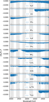 |
Fig. 2 Model isothermal spectra for each of the chemical species investigated in the atmosphere of HIP 67522 b. The gray shaded areas represent the wavelength coverage of CRIRES+ with six spectral orders, each spread over three detectors. |
3.2.2 Two temperature model
Because of the extremely high signal-to-noise ratio obtained in cross correlation maps, we decided to go a step further in the usual Bayesian analysis. We used a model with a discrete change in temperature in the atmosphere, which we call the ‘two-temperature model’. In the first step, we let the pressure at which this temperature change occur as a free parameter in the retrieval. We found that the retrieval favours a much higher deep temperature with a change between both temperatures favoured around a few mbar (2400 ± 400K in the interior, 1100 ± 100K above). The evidence ratio between this two-temperature model and the isothermal model amounts to 3 (see Sect. 4) and, thus, we find that the two-temperature model is not drastically favoured compared to an isothermal.
However, when we fixed the pressure at which the temperature change occurs to the best retrieved pressure (3 mbar), we obtained a similarly strong difference in temperature between the two parts of the atmosphere, but with a Bayes factor of 20. This shows that the data strongly favour a two-temperature model with a change at mbar pressures. We therefore re-estimated the metallicity and C/O ratio in the two-temperature model, displaying the result as an additional column in Table 1, as well as the abundances in Table 2. We also show the retrieved temperatures in Fig. 5. The corner plot of the posterior distribution for the two-temperature model is shown in Fig. B.1.
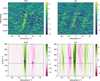 |
Fig. 3 Top panel: phase—vsys maps for the detected species H2O (left) and CO (right) in the stellar reference frame. The red dashed line indicates the predicted velocity trail of the planet. The colour bars are expressed in standard deviations away from both planet and telluric signals (excluding the square in the Kp-Vsys map defined by Kp ∈ [0,300] and Vsys ∈ [−10,30]). Bottom panel: Kp-vsys map for H2O (left) and CO (right), the vertical dashed line indicates the stellar reference frame, the horizontal dashed line indicates Kp = 120 km s−1. The maximum value of the map is indicated by the + symbol in black with the associated value, while the minimum is indicated by the blue cross. |
Molecular abundances from the isothermal and two-temperature retrievals.
3.2.3 Tentative detection of HDO
We searched for rarer molecules, namely, isotopologues of water and carbon monoxide. We searched for HDO, H218O, and 13CO. We were only able to put upper limits on H218O, and 13CO, but our retrieval favours the presence of HDO at 2σ. We searched for HDO in correlation maps, and we could not see a significant maximum of correlation from this molecule. We included HDO in our H2O models, but see no significant change in the maximum value in the correlation map is observed. However, the Bayes factor (see Sect. 4.2) for a model that includes HDO compared to a model with water and CO only is 12, indicating a strong preference towards a model that contains HDO.
The tentative detection of HDO in the atmosphere of HIP 67522 b yields a log10(HDO/H2O) = ∼1.4 ± 0.4, corresponding to a D/H enrichment factor of ∼1000 relative to the protosolar value. The implications of this high level of enrichment are discussed in Sect. 4.3.
To assess the robustness of the HDO detection, we ran injection-recovery tests where we injected our best-fit model in the data at -Kp and tried to retrieve the presence of HDO with correlation and nested sampling. Our results are highly consistent with the results on the real planet. In particular, we do not see anything striking out of the correlation map, but the HDO posterior from the nested sampling peaks at the injected value with a low MMR tail associated with lower likelihood (almost the same as to what is shown in Fig. 4). We also calculated the Bayes factor of a retrieval where we searched for both HDO and H2O, compared to a retrieval with only H2O, and as in the real data it is around 10. Finally, we injected a model with only water and tried to retrieve both water and HDO. We obtained a flat posterior with a 3σ limit on the MMR at 10−4.5, along with a Bayes factor of around 1 when we included (or not) HDO in the model. Essentially, our HDO detection is very strong statistically and perfectly consistent with the expectations of injection recovery tests.
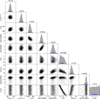 |
Fig. 4 Corner plot of the posterior distribution of our isothermal models. |
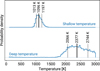 |
Fig. 5 Posterior distribution for the two-temperature model where the pressure change is fixed at 3 mbar. |
4 Discussion
The exceptionally high detection significance of H2O (20σ) and CO (5σ) in HIP 67522 b far exceeds typical values obtained through ground-based high-resolution IR transmission spectroscopy of hot Jupiters (e.g., Brogi et al. 2016; Birkby 2018). This remarkable signal strength directly reflects the planet’s extreme physical properties: its low mass combined with its inflated radius yields an atmospheric scale height comparable to the planetary radius itself, dramatically enhancing the transmission signal.
The velocity offset of ∼2.9 ± 0.2 km s−1 from the stellar systemic velocity indicates day-to-night atmospheric circulation, as expected for a highly irradiated planet. The upper limit on equatorial rotation (<2 km s−1 at 3σ) is consistent with tidal locking and excludes Jupiter-like rotation rates, suggesting that tidal dissipation can already have synchronised this young planet’s rotation with its orbital period. This is an important result for constraining star-planet tidal interactions.
Our derived C/O ratio of  (isothermal) and
  (two-temperature) indicates super-solar composition while our metallicity retrieval favours supersolar values or [C+O/H] of
  (isothermal) and
  (two-temperature). Our C/O ratio is in conflict with the work of Thao et al. (2024), where a solar C/O ratio was reported.
We note that our retrieved C/O and metallicity do not depend strongly on whether the mass uncertainty is included as a free parameter in the retrieval or is fixed; therefore, we remain confident that they represent correct values for our isothermal models no matter the mass. However, our metallicity is strongly dependent on the presence of clouds: the higher the clouds (up to 0.1 mbar, where they would hide the molecular signatures), the higher the metallicity. This degeneracy cannot be resolved by our data alone, but we note that there is no statistical preference for the presence of clouds as the Bayes factor is unity compared to a clear atmosphere (see Sect. 4.2). If we can validate an independent estimate of the metallicity and the mass, we will be able to infer whether the atmosphere is cloudy with a super solar metallicity or cloud free with a lower metal content. We also note that the presence of clouds has an effect on the mass but of only 10% at most (as clouds change the radius by a roughly similar amount), which does not resolve our discrepancy with Thao et al. (2024).
4.1 Mass constraints
The most puzzling result of our paper is the large discrepancy in mass with JWST observations, which are in disagreement at the 3σ level, favouring a planet that is twice as massive in our case. Unfortunately, without performing a joint JWST-CRIRES+ retrieval, which is beyond the scope of this paper, it is unlikely to resolve this issue. We can think of two possible flaws that might affect our results: (1) as we fit our radius to the TESS value, we could encounter an error if there is a strong optical absorber or a very large super-Rayleigh diffusion that would affect the deduced radius due to a much larger atmosphere than predicted in the visible. That would mean that the actual radius used in the gravity estimation is smaller, leading to a smaller mass for a given gravity. However, this is unlikely and it would need to affect a significant part of the large TESS wavelength range of integration (600-1100 nm roughly), but, on the other hand, this is not impossible; (2) in addition, our results depend on a normalisation factor, whose validity cannot be validated a posteriori. If there is a normalisation issue somewhere in our data analysis, it might explain the discrepancy.
If neither of these caveats make up the source of the discrepancy, then the atmospheric model can be the source of error. For example, the mass estimations from Thao et al. (2024) only used equilibrium chemistry models, whereas we ran free retrievals because we did not want to make assumptions on the thermodynamics of such young objects (which can be a source of discrepancy in the results). Essentially, with a complex temperature and/or composition profile, we might be able to reconcile CRIRES+ and JWST deduced masses (Chabrol et al., in prep.).
However, so long as the mass of the planet is unknown, the huge degeneracy that we obtain between mass, radius and reference pressure cannot be resolved (see Fig. 4). Combining with JWST might reduce the extent of this degeneracy, but it is pretty unlikely that it would actually resolve it. This unknown mostly affects the metallicity which is strongly dependent on the gravity through the scale height of the atmosphere and can only be poorly constrained thus far.
4.2 Bayes factor
In this paper, we compared several different atmospheric models, with different numbers for the free parameters. One usual way to perform model comparisons (and, hence, to decide whether a model is statistically favoured compared to another) in astrophysics is through the use of Bayesian (BIC) or Akaike information criterion (AIC), which are comparisons of the likelihoods of different models penalised by the number of parameters. A model that has a poor likelihood with very few parameters will often be preferred to a model that has a better fit but many more parameters. Such criteria are theoretical approaches to model comparison in the context of studies where the probability are defined relatively to an unknown multiplying factor in the Bayes equation (i.e. the evidence) that represents the probability of the data given a model. However, in the context of nested sampling, a measurement of the evidence is obtained as an output of the algorithm. We can thus use a more robust criterion for model comparison which is to calculate the evidence ratio (which is a statistical equivalent to Occam’s razor, see the detailed discussion in chapter 28 of Mackay 2003), also called the Bayes factor and often denoted as K,
 (5)
(5)
where D represents the data, M1 is a first model, and M2 the second. The rule of thumb criterion is to favour M1 over M2 when K>3, with a strong decision towards model 1 if K>10.
With our data, a model that contains water and CO compared to a model that only contains water leads to a Bayes factor of e22, which excludes with certainty the absence of CO in the atmosphere. Regarding the temperature structure, the two-temperature model with a free pressure transition is only slightly favoured over the isothermal model with a Bayes factor of 3. However, when fixing the pressure transition to the best retrieved value of 3 mbar, the Bayes factor reaches 20 in favour of the two-temperature model, indicating a strong statistical preference for a non-isothermal atmosphere. The HDO is also strongly favoured when using the evidence ratio.
4.3 HDO/H2O ratio as a possible signature of strong escape
The tentative 2σ detection of HDO would represent the first such measurement in an exoplanet atmosphere. It is associated with a Bayes factor of 12, which indicates a strong statistical preference towards the presence of this molecule in the atmosphere. However, if it is real, we must be able to explain the D/H enrichment factor of ∼1000 relative to the protosolar ratio. This enrichment is unlikely to arise from formation processes (Morley et al. 2019, and private comm. with C. Morley): such extreme deuterium fractionation largely exceeds the primordial ratio measured in protoplanetary disks (∼2 × 10⁻³; Tobin et al. 2023).
The only other known D/H ratio of such extreme value is in Venus’s atmosphere (log(HDO/H2O) ≈ −1.5; Donahue et al. 1982), where ∼4.5 Gyr of preferential hydrogen escape produced a ∼ 100-fold enrichment relative to Earth. Notably, a recent Venus Express analysis revealed that the venusian D/H ratio increases from ∼160 × terrestrial at the cloud tops to ∼1500 × at 108 km altitude (Mahieux et al. 2024), demonstrating that upper atmospheric layers can be significantly more enriched than the bulk atmosphere. As high-resolution transmission spectroscopy probes the upper atmosphere where photochemical fractionation and escape occur, our measurement might therefore reflect local fractionation in the escaping atmosphere, consistent with predictions that HDO could trace atmospheric evolution in irradiated exoplanets (Morley et al. 2019; Mollière et al. 2019).
For the 17 Myr old HIP 67522 b to achieve comparable enrichment than Venus would require extraordinarily rapid escape rates, plausibly driven by the intense XUV flux from its magnetically active, frequently flaring host star (Ilin et al. 2025b). Enhanced D/H ratios in exoplanet atmospheres due to atmospheric escape have been predicted by numerical models (e.g. Cherubim et al. 2024). The D/H ratio provides constraints on the atmospheric escape mechanism, particularly if the He/H ratio is measured as well, which allows us to distinguish between competing escape mechanisms. Follow-up observations at higher S/N values and different wavelength ranges are essential to confirm this detection. We also ought to further investigate whether young, highly irradiated planets routinely exhibit signatures of ongoing deuterium fractionation. Observations in the Y band near the He triplet at 1083 nm will eventually enable the measurement of He/H in cases where excess helium absorption is measured in the exoplanet atmosphere. Additionally, as pointed out by Cherubim et al. (2024), deuterium-enhanced planets should be helium-dominated and methane-depleted, meaning that there is a favourable wavelength range to detect HDO at 3.7 μm. This wavelength range is accessible to a few high-resolution spectrographs including CRIRES+ and iSHELL (Rayner et al. 2022), as well as the future Metis instrument at the Extremely Large Telescope (Brandl et al. 2021).
Data availability
The reduced data are available on Zenodo: https://doi.org/10.5281/zenodo.17909093 (Lavail et al. 2025). The raw data as well as the ESO-processed data are all publicly available one year after the observations at the ESO archive. The planet isothermal synthetic spectra (as well as associated information about opacity sources) are also available at the Zenodo record containing the reduced data.
Acknowledgements
Based on observations made with ESO Telescopes at the La Silla Paranal Observatory under programme ID 114.28HP. We are grateful to the ESO Director General and Director of Science for granting us DDT for this project, to the ESO observing staff, and to Michael Way and Caroline Morley for helpful discussions. F. Debras acknowledges funding from the French National Research Agency (ANR) project ExoATMO (ANR-25-CE49-6598). F. Debras would like to warmly thank the Action Thématique Physique Stellaire (ATPS) and Action Thématique ExoSystèmes (AT-EXOS) of CNRS/INSU cofunded by CEA and CNES for their financial support. B. Klein., S. Aigrain acknowledge funding from the European Research Council under the European Union’s Horizon 2020 research and innovation programme (grant agreement No. 865624, GPRV). A. Masson acknowledges support and funds from the grants no. CNS2023-144309 by the Spain Ministry of Science, Innovation and Universities MICIU/AEI/10.13039/501100011033. T. Hood acknowledges funding from the French National Research Agency (ANR) project EXOWINDS (ANR-23-CE31-0001-01). This work was granted access to the HPC resources of CALMIP supercomputing centre under the allocation 2021-p21021. This work made use of Astropy: a community-developed core Python package and an ecosystem of tools and resources for astronomy (Astropy Collaboration 2013, 2018, 2022), numpy (Harris et al. 2020). This research has made use of the Astrophysics Data System, funded by NASA under Cooperative Agreement 80NSSC21M0056. This research has made use of the SIMBAD database, operated at CDS, Strasbourg, France. The data reduction process was sped up thanks to GNU parallel (Tange 2023).
References
- Astropy Collaboration (Robitaille, T. P., et al.) 2013, A&A, 558, A33 [NASA ADS] [CrossRef] [EDP Sciences] [Google Scholar]
- Astropy Collaboration (Price-Whelan, A. M., et al.) 2018, AJ, 156, 123 [Google Scholar]
- Astropy Collaboration (Price-Whelan, A. M., et al.) 2022, ApJ, 935, 167 [NASA ADS] [CrossRef] [Google Scholar]
- Barber, M. G., Thao, P. C., Mann, A. W., et al. 2024, ApJ, 973, L30 [Google Scholar]
- Baruteau, C., Bai, X., Mordasini, C., & Mollière, P. 2016, Space Sci. Rev., 205, 77 [CrossRef] [Google Scholar]
- Birkby, J. L. 2018, in Handbook of Exoplanets, eds. H. J. Deeg, & J. A. Belmonte, 16 [Google Scholar]
- Blain, D., Mollière, P., & Nasedkin, E. 2024, J. Open Source Softw., 9, 7028 [Google Scholar]
- Brandl, B., Bettonvil, F., van Boekel, R., et al. 2021, The Messenger, 182, 22 [NASA ADS] [Google Scholar]
- Brogi, M., & Line, M. R. 2019, AJ, 157, 114 [Google Scholar]
- Brogi, M., de Kok, R. J., Albrecht, S., et al. 2016, ApJ, 817, 106 [Google Scholar]
- Buchner, J., Georgakakis, A., Nandra, K., et al. 2014, A&A, 564, A125 [NASA ADS] [CrossRef] [EDP Sciences] [Google Scholar]
- Cherubim, C., Wordsworth, R., Hu, R., & Shkolnik, E. 2024, ApJ, 967, 139 [Google Scholar]
- David, T. J., Petigura, E. A., Luger, R., et al. 2019, ApJ, 885, L12 [Google Scholar]
- Debras, F., Klein, B., Donati, J.-F., et al. 2024, MNRAS, 527, 566 [Google Scholar]
- Donahue, T. M., Hoffman, J. H., Hodges, R. R., & Watson, A. J. 1982, Science, 216, 630 [NASA ADS] [CrossRef] [Google Scholar]
- Dorn, R. J., Bristow, P., Smoker, J. V., et al. 2023, A&A, 671, A24 [NASA ADS] [CrossRef] [EDP Sciences] [Google Scholar]
- Feroz, F., & Hobson, M. P. 2008, MNRAS, 384, 449 [NASA ADS] [CrossRef] [Google Scholar]
- Feroz, F., Hobson, M. P., & Bridges, M. 2009, MNRAS, 398, 1601 [NASA ADS] [CrossRef] [Google Scholar]
- Gibson, N. P., Merritt, S., Nugroho, S. K., et al. 2020, MNRAS, 493, 2215 [Google Scholar]
- Gibson, N. P., Nugroho, S. K., Lothringer, J., Maguire, C., & Sing, D. K. 2022, MNRAS, 512, 4618 [NASA ADS] [CrossRef] [Google Scholar]
- Harris, C. R., Millman, K. J., van der Walt, S. J., et al. 2020, Nature, 585, 357 [NASA ADS] [CrossRef] [Google Scholar]
- Heitzmann, A., Zhou, G., Quinn, S. N., et al. 2021, ApJ, 922, L1 [NASA ADS] [CrossRef] [Google Scholar]
- Hood, T., Debras, F., Moutou, C., et al. 2024, A&A, 687, A119 [NASA ADS] [CrossRef] [EDP Sciences] [Google Scholar]
- Ilin, E., Bloot, S., Callingham, J. R., & Vedantham, H. K. 2025a, A&A, 699, A147 [NASA ADS] [CrossRef] [EDP Sciences] [Google Scholar]
- Ilin, E., Vedantham, H. K., Poppenhäger, K., et al. 2025b, Nature, 643, 645 [Google Scholar]
- Kanodia, S., & Wright, J. 2018, RNAAS, 2, 4 [NASA ADS] [Google Scholar]
- Klein, B., Debras, F., Donati, J.-F., et al. 2024, MNRAS, 527, 544 [Google Scholar]
- Lavail, A., Debras, F., & Klein, B. 2025, https://doi.org/10.5281/zenodo.17909093 [Google Scholar]
- Mackay, D. J. C. 2003, Information Theory, Inference and Learning Algorithms (Cambridge University Press) [Google Scholar]
- Mahieux, A., Viscardy, S., Yelle, R. V., et al. 2024, PNAS, 121, e2401638121 [Google Scholar]
- Mann, A. W., Newton, E. R., Rizzuto, A. C., et al. 2016, AJ, 152, 61 [Google Scholar]
- Mann, A. W., Wood, M. L., Schmidt, S. P., et al. 2022, AJ, 163, 156 [NASA ADS] [CrossRef] [Google Scholar]
- Mollière, P., Wardenier, J. P., van Boekel, R., et al. 2019, A&A, 627, A67 [Google Scholar]
- Morley, C. V., Skemer, A. J., Miles, B. E., et al. 2019, ApJ, 882, L29 [NASA ADS] [CrossRef] [Google Scholar]
- Nortmann, L., Lesjak, F., Yan, F., et al. 2025, A&A, 693, A213 [NASA ADS] [CrossRef] [EDP Sciences] [Google Scholar]
- Owen, J. E. 2019, Annu. Rev. Earth Planet. Sci., 47, 67 [CrossRef] [Google Scholar]
- Plavchan, P., Barclay, T., Gagné, J., et al. 2020, Nature, 582, 497 [Google Scholar]
- Rackham, B. V., Apai, D., & Giampapa, M. S. 2018, ApJ, 853, 122 [Google Scholar]
- Rayner, J., Tokunaga, A., Jaffe, D., et al. 2022, PASP, 134, 015002 [NASA ADS] [CrossRef] [Google Scholar]
- Rizzuto, A. C., Newton, E. R., Mann, A. W., et al. 2020, AJ, 160, 33 [Google Scholar]
- Snellen, I. A. G., de Kok, R. J., de Mooij, E. J. W., & Albrecht, S. 2010, Nature, 465, 1049 [Google Scholar]
- Tange, O. 2023, https://doi.org/10.5281/zenodo.10199085 [Google Scholar]
- Thao, P. C., Mann, A. W., Feinstein, A. D., et al. 2024, AJ, 168, 297 [Google Scholar]
- Tobin, J. J., van’t Hoff, M. L. R., Leemker, M., et al. 2023, Nature, 615, 227 [NASA ADS] [CrossRef] [Google Scholar]
The reference pressure is the pressure where the gravity is equal to the input gravity, and hence the radius is equal to the one used in the code (here 0.892 Jupiter radii).
Appendix A Cross-correlation maps for non-detected species
Appendix B Posterior distribution for the two-temperature models
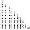 |
Fig. B.1 Corner plot of the posterior distribution of our two-temperature models. |
All Tables
All Figures
|
Fig. 1 Evolution of the transit window, the median S/N per exposure, seeing, and airmass as a function of time from the first exposure. The median S/N and median seeing for the full time-series are indicated in red on the second and third panel respectively. The UT time at the start of the first exposure t0 is indicated on the fourth panel. |
| In the text | |
|
Fig. 2 Model isothermal spectra for each of the chemical species investigated in the atmosphere of HIP 67522 b. The gray shaded areas represent the wavelength coverage of CRIRES+ with six spectral orders, each spread over three detectors. |
| In the text | |
|
Fig. 3 Top panel: phase—vsys maps for the detected species H2O (left) and CO (right) in the stellar reference frame. The red dashed line indicates the predicted velocity trail of the planet. The colour bars are expressed in standard deviations away from both planet and telluric signals (excluding the square in the Kp-Vsys map defined by Kp ∈ [0,300] and Vsys ∈ [−10,30]). Bottom panel: Kp-vsys map for H2O (left) and CO (right), the vertical dashed line indicates the stellar reference frame, the horizontal dashed line indicates Kp = 120 km s−1. The maximum value of the map is indicated by the + symbol in black with the associated value, while the minimum is indicated by the blue cross. |
| In the text | |
|
Fig. 4 Corner plot of the posterior distribution of our isothermal models. |
| In the text | |
|
Fig. 5 Posterior distribution for the two-temperature model where the pressure change is fixed at 3 mbar. |
| In the text | |
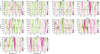 |
Fig. A.1 Same as Fig. 3 but for all the non-detected species. |
| In the text | |
|
Fig. B.1 Corner plot of the posterior distribution of our two-temperature models. |
| In the text | |
Current usage metrics show cumulative count of Article Views (full-text article views including HTML views, PDF and ePub downloads, according to the available data) and Abstracts Views on Vision4Press platform.
Data correspond to usage on the plateform after 2015. The current usage metrics is available 48-96 hours after online publication and is updated daily on week days.
Initial download of the metrics may take a while.