| Issue |
A&A
Volume 710, June 2026
|
|
|---|---|---|
| Article Number | L18 | |
| Number of page(s) | 9 | |
| Section | Letters to the Editor | |
| DOI | https://doi.org/10.1051/0004-6361/202660461 | |
| Published online | 12 June 2026 | |
Letter to the Editor
Seismic signature of a magnetic field in the γ Doradus star KIC 2309579
1
IRAP, Université de Toulouse, CNRS, CNES, 14 avenue Edouard Belin, 31400 Toulouse, France
2
Max-Planck-Institut für Sonnensystemforschung, 37077 Göttingen, Germany
3
Centre for Astrophysics, University of Southern Queensland, Toowoomba, QLD 4350, Australia
★ Corresponding author: This email address is being protected from spambots. You need JavaScript enabled to view it.
Received:
16
April
2026
Accepted:
21
May
2026
Abstract
Context. Internal magnetic fields have recently been detected and measured in the radiative core of red giant stars using asteroseismology. As they are one of the progenitors of red giant stars and exhibit high radial order gravity modes, γ Doradus stars may also hold detectable magnetic fields in their radiative envelope.
Aims. We aim to detect, for the first time, an internal magnetic field in a rapidly rotating γ Doradus star through its influence on the propagation of Kelvin gravito-inertial modes.
Methods. We used the seismic variable δKa, defined as a combination of Kelvin modes frequencies, which is sensitive to the presence of a magnetic field. Following the detection, we modeled the star oscillation spectrum while considering a magnetic component following a Bayesian approach.
Results. We found a magnetic signature in the radiative envelope of KIC 2309579. If located just above the core, in the layers that were previously convective, the magnetic field would reach ∼4 kG.
Key words: asteroseismology / stars: magnetic field / stars: oscillations / stars: individual: KIC 2309579
© The Authors 2026
 Open Access article, published by EDP Sciences, under the terms of the Creative Commons Attribution License (https://creativecommons.org/licenses/by/4.0), which permits unrestricted use, distribution, and reproduction in any medium, provided the original work is properly cited.
This article is published in open access under the Subscribe to Open model. This email address is being protected from spambots. You need JavaScript enabled to view it. to support open access publication.
1. Introduction
Over the past few decades, asteroseismology has emerged as a powerful tool for probing the interior of stars, and it has revealed crucial measurements of near-core rotations, ages, and masses. These measurements have shown that stellar models overestimate core rotation (Mosser et al. 2012; Ouazzani et al. 2019), which indicates that some physical phenomenon occurring in stars are missing in our models. Magnetic fields may be a major actor in the angular momentum transport within stars. Nevertheless, for a long time, only surface magnetic fields could be detected and studied using spectropolarimetry, leaving the study of the inner part of the fields inaccessible. Fuller et al. (2015) showed that a strong enough inner magnetic field hinders the propagation of gravity (g) modes and could explain the suppression of mixed dipolar modes observed in some red giants stars. More recently, magnetic fields have been detected and measured in the radiative core of several red giants stars (Li et al. 2022, 2023; Deheuvels et al. 2023; Hatt et al. 2024; Villate et al. 2026) and in the radiative envelope of a slowly rotating δ Scuti-γ Doradus star (Takata et al. 2026) using a seismic approach. These measurements provide key constraints for answering the question of angular momentum transport. The γ Doradus (γ Dor) stars are pulsating main-sequence (MS) late A- to early F-type stars with masses from 1.3 to 2 M⊙ (Kaye et al. 1999). Their internal structure is composed of a convective core, a radiative envelope, and a shallow convective envelope. Although they exhibit high radial order gravito-inertial (g − i) modes, which are most affected by magnetic fields, there is currently no seismic evidence of inner magnetic fields in the typical rapidly rotating γ Dor stars. Their rotation periods, which are on the order of a day (Li et al. 2020), make it impossible to consider rotation as a perturbation, as is done for red giants (Li et al. 2022). The traditional approximation of rotation (Lee & Saio 1997), hereafter referred to as “TAR”, has been used instead to study g − i modes of rapidly rotating stars, as its validity has been tested for the modes observed in γ Dor stars (Ballot et al. 2012; Ouazzani et al. 2017, 2020). Prat et al. (2019, 2020) studied the effect of dipolar magnetic fields on TAR g − i modes considering the Lorentz force as a perturbation, while Dhouib et al. (2022) treated the Lorentz force in a nonperturbative way for an axisymetric toroidal field. Recently, Lignières et al. (2024) proposed a generalization to an arbitrary magnetic field of the perturbative approach and derived analytical forms of frequency shifts for g − i and Rossby modes. They also introduced a new seismic variable, which is specifically sensitive to magnetic fields: the difference of Kelvin mode frequencies δKa.
In the following, we first present the method for identifying magnetic star candidates thanks to the seismic variable δKa and carry out the spectral analysis of such a star, KIC 2309579, in Sect. 2. We then present the modeling of the star oscillation spectrum considering a magnetic component as well as the corresponding results in Sect. 3. In Sect. 4, we investigate the properties of the inner magnetic field of KIC 2309579. Finally, we present a discussion and a conclusion in Sect. 5.
2. Identifying magnetic candidates
Kelvin modes are g − i equatorial prograde modes present in rotating stars. They are usually labeled by their degree ℓ and their azimuthal order m = −ℓ, as they become prograde sectoral modes at zero rotation. Lignières et al. (2024) have introduced a seismic variable, δKa, defined as a combination between the frequencies of ℓ = 1 and ℓ = 2 Kelvin modes with the same radial order n, denoted νn, ℓ, normalized by twice the star rotation frequency νrot:
 (1)
(1)
In the absence of a magnetic field, asymptotic theory predicts that δKa is the same function of the spin parameter  , where
  refers to the νn, ℓ frequency in the corotation frame, for all γ Dor stars and that this function vanishes at high sn, 1. In contrast, the radial component of a magnetic field produces an increase of δKa proportional to sn, 13. This property provides a simple method for detecting magnetic fields in γ Dor stars holding both ℓ = 1 and ℓ = 2 Kelvin modes.
2.1. Description of the analyzed γ Dor star sample
Li et al. (2020) analyzed 611 γ Dor stars observed by the Kepler space mission (Borucki et al. 2010). They found both ℓ = 1 and ℓ = 2 Kelvin modes among 155 of these stars. From a ΔP − P diagram fitting method, they determined the rotation frequencies and the buoyancy radii Π0 of these stars. We identified the radial order of modes detected in these stars with the TAR and computed δKa for this sample. Results are shown in Fig. 1. The data collapse around a single curve, independent of the rotation rate of the stars, that converges at high spin parameters toward the asymptotic relation calculated within the TAR and the Wentzel-Kramers-Brillouin (WKB) approximation, denoted δKTh. We thus searched for stars showing deviations from this general trend. Some points exhibit strong departures, but we have shown it is generally due to incorrect radial order identifications. We identified a few stars with a behavior compatible with what we expect from a magnetic field. In the rest of the paper, we present the detailed analysis of the best candidate, KIC 2309579.
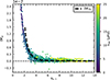 |
Fig. 1. Dimensionless seismic variable δKa as a function of the spin parameter sn, 1 for the 155 γ Dor stars from the Li et al. (2020) catalog. A dashed black curve shows the asymptotic approximation δKTh (see Lignières et al. 2024). Colors indicate the stellar rotation rate. |
2.2. Spectral analysis of KIC 2309579
In order to fully control all the steps of the analysis, we first reprocessed the Kepler light curve of KIC 2309579 downloaded from the MAST archive1 in order to extract the oscillation frequencies using the FELIX code (Charpinet et al. 2010; Zong et al. 2016). We extracted the frequencies with a signal-to-noise ratio greater than 4.7, that is a 4σ detection level. The detailed result of the extraction is reported in Appendix D. As in Li et al. (2020), we identified ℓ = 1 and ℓ = 2 Kelvin modes in the ranges 13–17 μHz and 28–32 μHz. The mode identification was performed with the GMorse code (Christophe et al. 2018).
We excluded from the following analysis the frequencies that have high probabilities (≤2σ) to be linear combinations of two higher amplitude frequencies or harmonics of higher peaks. Figure 2 shows the δKa of KIC 2309579 computed from this frequency list. For comparison, also plotted are the median δKa of the 155 stars and δKTh. The values measured for KIC 2309579 exhibit a clear departure from the median of the whole sample and from δKTh. Furthermore, we found that this departure is compatible with a profile proportional to sn, 13, as expected for magnetic stars. The difference between δKTh and the median δKa can be partly explained by the limitations of the asymptotic theory (Lignières et al. 2024), but it could also result from a general magnetic behavior of the star sample. The small oscillatory behavior of the data is likely due to a glitch occurring near the convective core of the star. The variable δKa is a good indicator of a candidate, but it has limitations: (i) Its results rely on an a priori determination of n, which can be biased by the presence of a magnetic field (Lignières et al. 2024). (ii) We only used 20 out of the 34 extracted frequencies (those that share a common n and have a different ℓ). In the following, we propose using a magnetic model to reproduce KIC 2309579 oscillation spectrum.
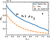 |
Fig. 2. Dimensionless seismic variable δKa as a function of the spin parameter sn, 1 for modes identified in KIC 2309579. For comparison, we plot the median δKa of the 155 stars (blue line) and the asymptotic approximation δKTh (orange dashes). |
3. Spectrum model including magnetic field
Following an approach similar to the one used to analyze red giant stars by Villate et al. (2026), we fit all the observed mode frequencies with an asymptotic model that includes the effects of a magnetic field. We present the model in Sect. 3.1 and the results of the fit to the observations in Sect. 3.2.
3.1. Asymptotic model
In the absence of a magnetic field, we computed the frequencies of Kelvin modes within the TAR and used the WKB approximation in the radial direction. In this case, the non-perturbed frequencies νn, ℓ0 of modes are expressed through the equation
 (2)
(2)
where Λℓ(s) are the Laplace tidal equation eigenvalues, Π0 is the buoyancy radius of the star, and ϵgℓ is a phase offset for modes of degree ℓ (e.g., Berthomieu et al. 1978). Lignières et al. (2024) derived the perturbation of frequencies induced by a magnetic field not dominated by its azimuthal component for ℓ = 1 and ℓ = 2 Kelvin modes:
 (3)
(3)
where  in the cgs system, with
 (4)
(4)
 (5)
(5)
where ρ is the density, N the Brunt-Väisälä frequency, and ri and ro are respectively the inner and outer boundaries of the oscillation cavity. The factor ℐ depends on the stellar structure along the oscillation cavity and Beq2 is the radial and azimuthal average of the radial component of the magnetic field evaluated at the equator, where Kelvin modes are mainly concentrated for large spin parameters. The radial weight function, Kr(r), is defined as
 (6)
(6)
Compared to Eqs. (30) and (31) in Lignières et al. (2024), we left out a ∝1/s term that appears to be negligible in front of the first-order terms. The model thus relies on five free parameters: Π0, νrot, ϵg1, ϵg2, and νB.
3.2. Fitting the model to observations
We fit our model to the observed frequencies by following a Bayesian approach using the ABIM code (see Appendix A.2 for details). We obtained unimodal (almost normal) posterior distributions for all parameters. We compared the best-model frequencies, obtained from the median values of these distributions, to the observed ones. We plot the comparison in a so-called stretched period échelle diagram (Christophe et al. 2018) in Fig. 3. The best model is consistent with the observations. In a nonmagnetic TAR framework, the échelle diagrams represent mode periods sharing the same ℓ and m on a vertical line. In our case, the échelle diagrams, especially that of the ℓ = 1 modes, show distinct curvatures due to the influence of the magnetic field on the higher periods. In the plot, we display the frequencies we excluded from the analysis, because they could be interpreted as frequency combinations. Some of them could nevertheless be modes since they are very close to modeled frequencies.
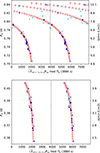 |
Fig. 3. Stretched period échelle diagram of ℓ = 1 (top) and ℓ = 2 (bottom) Kelvin mode frequencies. Navy blue dots indicate observed frequencies used for the analysis. Light blue dots represent observed frequencies that are possible frequency combinations and discarded for the analysis. Red circles are frequencies of the best model including a magnetic field. The size of the dots is proportional to the mode amplitude. |
We then derived the posterior distribution of ℐBeq2 from those of νB and νrot. We thus measured that ℐBeq2 = 2.23 ± 0.16 × 10⁻²⁰ cm s−2 g−1 G2. In order to infer a magnetic field strength, we needed a stellar structure model of KIC 2309579.
4. Magnetic field strength
We computed γ Dor star models with CESAM2k20 (Morel 1997; Manchon et al. 2025) calibrated on the buoyancy radius of KIC 2309579 that we measured as well as its luminosity, effective temperature, and metallicity observed by Gaia (Gaia Collaboration 2023). We considered different mixing lengths in the convective envelope and different overshoot and mixing prescriptions above the core (see Appendix C). The weight function, Kr, peaks in two regions in our models: above the convective core, where composition gradients are strong, and below the convective envelope (see Fig. C.1). From one model to another, the relative contribution of these two regions may change significantly. Indeed, when the convective envelope is shallower, the weight of the upper layers increases. As a consequence, ℐ varies from one model to another, and the measured magnetic field averaged over the radiative region ranges from 140 to 590 G. To go further, since Kr(r) is bimodal, we needed to consider two possibilities: (i) the field is located below the convective envelope or (ii) it is located above the core.
In the first case, an average magnetic field Br ≈ 140 − 700 G below the envelope reproduces the observed signature. However, such a field appears to be larger by an order of magnitude than the critical field in this region (see an example in Fig. C.2). Such a magnetic field would be strong enough to suppress g modes (Fuller et al. 2015). Thus, we ruled out this possibility.
For the second scenario, we assumed that a magnetic field is present in the layers above the core that were previously convective. This field is thought to be a remnant of the convective core dynamo-generated field that was left behind when the convective core retreated. In this case, a field Br = 4 ± 0.3 kG reproduces the observed signature. The error bar reflects the dependence on the star models of KIC 2309579. Moreover, we verified that the value of Br is below the critical field for all the star models. Therefore, this second scenario is clearly favored.
5. Discussion and conclusion
If the presence of a magnetic field perfectly explains the spectrum of KIC 2309579, we must verify that other phenomena cannot mimic the signature of a magnetic field. We especially considered the presence of glitches, differential rotation, and dips induced by pure inertial modes in the core.
Glitches are expected to occur in γ Dor stars due to the sharp increase of the Brunt-Väisälä frequency above the convective core. However, following Miglio et al. (2008), the frequency shift induced by a glitch for a ℓ = 2 Kelvin mode is twice the shift for the ℓ = 1 Kelvin mode with the same radial order. As a consequence, glitches tend to vanish in δKa and cannot explain the observed signature.
The effects of radial differential rotation have been studied by Takata et al. (2020). They showed it can be treated within the TAR by considering a rotation that is an average over the mode cavity, which is the same for ℓ = 1 and 2 Kelvin modes. Moreover, since the latitudinal variation of ℓ = 1 and ℓ = 2 Kelvin modes are very similar (see, e.g., Lignières et al. 2024), we expect that latitudinal differential rotation affects ℓ = 1 and ℓ = 2 Kelvin modes similarly and cancel out in δKa.
Finally, in the range of spin parameters reached in this study, ℓ = 1 Kelvin modes could couple with a purely inertial mode propagating in the convective core, creating a so-called dip (Ouazzani et al. 2020). This induces frequency shifts of modes, creating a feature in δKa that could mimic the one produced by a magnetic field. We thus decided to model the spectrum of KIC 2309579 by considering the presence of a dip, following Tokuno & Takata (2022) and Galoy et al. (2024). Results are presented in Appendix B. The model struggles to reproduce both ℓ = 1 and ℓ = 2 long-period modes, whereas the magnetic model explains the whole spectra well (see Fig. B.1). Moreover, the coupling factor q between the pure inertial mode and g − i modes is large, reaching values that are expected for early MS stars (Galoy et al. 2024), whereas KIC 2309579 is a mid-MS star, according to our models and the models of Fritzewski et al. (2024). In addition, the spin parameter of the inertial mode s★ has values that are lower than the expected ones (Galoy et al. 2024). To explain this, we could invoke a fast rotating core or the presence of a strong magnetic field inside the core (Barrault et al. 2025a,b). However, in such a case, a decrease of s★ must be accompanied by a strong decrease of q, which contradicts the observation. We conclude that a dip hardly reproduces the spectrum of KIC 2309579.
We thus detected a near-core magnetic field of Br ≈ 4 kG in KIC 2309579. This is the first seismic evidence of a magnetic field in a typical γ Dor star, as the detection by Takata et al. (2026) concerns a star that rotates abnormally slowly for a γ Dor star. Li et al. (2022) proposed that magnetic fields observed in the core of red giants were remnants of core magnetic fields of the MS. The field strength extrapolated by Li et al. (2022) for MS stars is similar to the one found in this paper and in Takata et al. (2026), which is compatible with a convective core dynamo field. The technique we used to analyze this star will be extended to other γ Dor stars observed by spaced-based missions such as Kepler, TESS, and, in the very near future, PLATO.
Acknowledgments
We thank the anonymous referee for providing helpful and constructive comments. This work has been supported by CNES, focused on the preparation of the PLATO mission. We thanks M. Deal for his useful advice on stellar modeling, O. Creevey for her precious insight on Gaia measurements, and V. Antoci for useful discussion on spectral analysis. This paper includes data collected by the Kepler mission and obtained from the MAST data archive at the Space Telescope Science Institute (STScI). Funding for the Kepler mission is provided by the NASA Science Mission Directorate. STScI is operated by the Association of Universities for Research in Astronomy, Inc., under NASA contract NAS 5–26555.
References
- Alecian, G., & LeBlanc, F. 2020, MNRAS, 498, 3420 [NASA ADS] [CrossRef] [Google Scholar]
- Angulo, C., Arnould, M., Rayet, M., et al. 1999, Nucl. Phys. A, 656, 3 [Google Scholar]
- Asplund, M., Grevesse, N., Sauval, A. J., & Scott, P. 2009, ARA&A, 47, 481 [NASA ADS] [CrossRef] [Google Scholar]
- Ballot, J., Lignières, F., Prat, V., Reese, D. R., & Rieutord, M. 2012, ASPC Ser., 462, 389 [Google Scholar]
- Barrault, L., Mathis, S., & Bugnet, L. 2025a, A&A, 694, A225 [NASA ADS] [CrossRef] [EDP Sciences] [Google Scholar]
- Barrault, L., Bugnet, L., Mathis, S., & Mombarg, J. S. G. 2025b, A&A, 701, A253 [NASA ADS] [CrossRef] [EDP Sciences] [Google Scholar]
- Benomar, O., Appourchaux, T., & Baudin, F. 2009, A&A, 506, 15 [NASA ADS] [CrossRef] [EDP Sciences] [Google Scholar]
- Berthomieu, G., Gonczi, G., Graff, P., Provost, J., & Rocca, A. 1978, A&A, 70, 597 [Google Scholar]
- Böhm-Vitense, E. 1958, Z. Astrophys., 46, 108 [Google Scholar]
- Borucki, W. J., Koch, D., Basri, G., et al. 2010, Science, 327, 977 [Google Scholar]
- Charpinet, S., Green, E. M., Baglin, A., et al. 2010, A&A, 516, L6 [NASA ADS] [CrossRef] [EDP Sciences] [Google Scholar]
- Christophe, S., Ballot, J., Ouazzani, R.-M., Antoci, V., & Salmon, S. J. A. J. 2018, A&A, 618, A47 [NASA ADS] [CrossRef] [EDP Sciences] [Google Scholar]
- Deheuvels, S., Li, G., Ballot, J., & Lignières, F. 2023, A&A, 670, L16 [NASA ADS] [CrossRef] [EDP Sciences] [Google Scholar]
- Dhouib, H., Mathis, S., Bugnet, L., Van Reeth, T., & Aerts, C. 2022, A&A, 661, A133 [NASA ADS] [CrossRef] [EDP Sciences] [Google Scholar]
- Fritzewski, D. J., Aerts, C., Mombarg, J. S. G., Gossage, S., & Van Reeth, T. 2024, A&A, 684, A112 [NASA ADS] [CrossRef] [EDP Sciences] [Google Scholar]
- Fuller, J., Cantiello, M., Stello, D., Garcia, R. A., & Bildsten, L. 2015, Science, 350, 423 [Google Scholar]
- Gaia Collaboration (Vallenari, A., et al.) 2023, A&A, 674, A1 [NASA ADS] [CrossRef] [EDP Sciences] [Google Scholar]
- Galoy, M., Lignières, F., & Ballot, J. 2024, A&A, 689, A177 [NASA ADS] [CrossRef] [EDP Sciences] [Google Scholar]
- Goodman, J., & Weare, J. 2010, Commun. Appl. Math. Comp. Sci., 5, 65 [NASA ADS] [CrossRef] [Google Scholar]
- Hatt, E. J., Ong, J. M. J., Nielsen, M. B., et al. 2024, MNRAS, 534, 1060 [NASA ADS] [CrossRef] [Google Scholar]
- Imbriani, G., Costantini, H., Formicola, A., et al. 2004, A&A, 420, 625 [NASA ADS] [CrossRef] [EDP Sciences] [Google Scholar]
- Kaye, A. B., Handler, G., Krisciunas, K., Poretti, E., & Zerbi, F. M. 1999, PASP, 111, 840 [Google Scholar]
- Lee, U., & Saio, H. 1997, ApJ, 491, 839 [Google Scholar]
- Li, G., Van Reeth, T., Bedding, T. R., et al. 2020, MNRAS, 491, 3586 [Google Scholar]
- Li, G., Deheuvels, S., Ballot, J., & Lignières, F. 2022, Nature, 610, 43 [NASA ADS] [CrossRef] [Google Scholar]
- Li, G., Deheuvels, S., Li, T., Ballot, J., & Lignières, F. 2023, A&A, 680, A26 [NASA ADS] [CrossRef] [EDP Sciences] [Google Scholar]
- Lignières, F., Ballot, J., Deheuvels, S., & Galoy, M. 2024, A&A, 683, A2 [NASA ADS] [CrossRef] [EDP Sciences] [Google Scholar]
- Manchon, L., Deal, M., Marques, J. P. C., & Lebreton, Y. 2025, A&A, 704, A79 [Google Scholar]
- Michaud, G., & Proffitt, C. R. 1993, ASPC Ser., 40, 246 [Google Scholar]
- Miglio, A., Montalbán, J., Noels, A., & Eggenberger, P. 2008, MNRAS, 386, 1487 [Google Scholar]
- Mombarg, J. S. G., Van Reeth, T., & Aerts, C. 2021, A&A, 650, A58 [NASA ADS] [CrossRef] [EDP Sciences] [Google Scholar]
- Morel, P. 1997, A&AS, 124, 597 [NASA ADS] [CrossRef] [EDP Sciences] [Google Scholar]
- Morel, P., & Lebreton, Y. 2008, Ap&SS, 316, 61 [Google Scholar]
- Mosser, B., Goupil, M. J., Belkacem, K., et al. 2012, A&A, 548, A10 [NASA ADS] [CrossRef] [EDP Sciences] [Google Scholar]
- Ouazzani, R.-M., Salmon, S. J. A. J., Antoci, V., et al. 2017, MNRAS, 465, 2294 [Google Scholar]
- Ouazzani, R.-M., Marques, J. P., Goupil, M.-J., et al. 2019, A&A, 626, A121 [NASA ADS] [CrossRef] [EDP Sciences] [Google Scholar]
- Ouazzani, R.-M., Lignières, F., Dupret, M.-A., et al. 2020, A&A, 640, A49 [EDP Sciences] [Google Scholar]
- Prat, V., Mathis, S., Buysschaert, B., et al. 2019, A&A, 627, A64 [NASA ADS] [CrossRef] [EDP Sciences] [Google Scholar]
- Prat, V., Mathis, S., Neiner, C., et al. 2020, A&A, 636, A100 [NASA ADS] [CrossRef] [EDP Sciences] [Google Scholar]
- Reese, D., Rieutord, M., & Lignières, F. 2006, A&A, 455, 607 [NASA ADS] [CrossRef] [EDP Sciences] [Google Scholar]
- Richer, J., Michaud, G., & Turcotte, S. 2000, ApJ, 529, 338 [Google Scholar]
- Rogers, F. J., & Nayfonov, A. 2002, ApJ, 576, 1064 [Google Scholar]
- Serenelli, A. M. 2010, Ap&SS, 328, 13 [Google Scholar]
- Takata, M., Ouazzani, R.-M., Saio, H., et al. 2020, A&A, 635, A106 [NASA ADS] [CrossRef] [EDP Sciences] [Google Scholar]
- Takata, M., Murphy, S. J., Kurtz, D. W., Saio, H., & Shibahashi, H. 2026, MNRAS, 545, staf2153 [Google Scholar]
- Tokuno, T., & Takata, M. 2022, MNRAS, 514, 4140 [NASA ADS] [CrossRef] [Google Scholar]
- Townsend, R. H. D., & Teitler, S. A. 2013, MNRAS, 435, 3406 [Google Scholar]
- Verma, K., & Silva Aguirre, V. 2019, MNRAS, 489, 1850 [NASA ADS] [CrossRef] [Google Scholar]
- Villate, M., Deheuvels, S., & Ballot, J. 2026, A&A, 707, A366 [NASA ADS] [CrossRef] [EDP Sciences] [Google Scholar]
- Zong, W., Charpinet, S., Vauclair, G., Giammichele, N., & Van Grootel, V. 2016, A&A, 585, A22 [NASA ADS] [CrossRef] [EDP Sciences] [Google Scholar]
Appendix A: Magnetic model spectrum
A.1. Asymptotic magnetic model
As described in Sect. 3.1, we modeled the spectrum of KIC 2309579 within an asymptotic approximation of the TAR. Christophe et al. (2018) have shown that the asymptotic TAR is well suited to model g-i mode spectra of rotating stars. Of course, there are some deviations due to non-asymptotic effects, and we must ensure that these deviations do not introduce biases that could lead to false magnetic detections. We then used spectra computed with the 2D oscillation code TOP (Reese et al. 2006) that was used in Lignières et al. (2024), as well as spectra computed with the non-asymptotic TAR oscillation code GYRE (Townsend & Teitler 2013). We computed spectra of a γ Dor star model with a mass of 1.5 M⊙ and a radius 2.2 R⊙ with a rotation of 11.5μHz. We then fitted our asymptotic model of ℓ = 1 and ℓ = 2 Kelvin modes to these synthetic spectra. We found good agreement. We are able to fit simultaneously both series of modes with a common Π0 and νrot by allowing two different values for the phase offset ϵg. Values of ϵg, 1 and ϵg, 2 are very close but need to be slightly different to correctly reproduce the spectra. We then added νB as a free parameter in the asymptotic model. We fitted our synthetic spectra and verified we recover a value of νB compatible with zero.
Similarly to Villate et al. (2026), we decided to introduce a model error, which is quadratically added to the observation errors, to take into account the dispersion of frequencies around the asymptotic model due to non-asymptotic effects. Based on a comparison of asymptotic models to complete computations, we have considered that, for each series of modes, the error of periods is constant in the corotation frame. We thus added two additional free parameters, σℓ1 and σℓ2, which are the model error of ℓ = 1 and ℓ = 2 Kelvin modes.
A.2. Fitting the observations
We fit our model to the observed frequencies by following a Bayesian approach with a Markov chain Monte Carlo (MCMC) method. We defined priors for all parameters of the model. The prior for buoyancy radius Π0 follows a uniform distribution over [3000, 5000] seconds, which covers the typical Π0 values for γ Dor stars (Li et al. 2020). Li et al. (2020) also showed that the seismic rotation period remains quite close to the surface one for γ Dor stars. As KIC 2309579 exhibits a rotational modulation at 11.50μHz (see Appendix D), we set a uniform prior distribution over [11, 12] μHz for νrot. We set a uniform-periodic prior distribution over [0, 1] for the ϵg1 and ϵg2 parameters. Here, “uniform-periodic” means a uniform prior for which the posteriors are the results of steps by the walkers modulo the interval range. As we do not have prior information about the magnetic component νB, we used a non-informative distribution, the modified Jeffrey distribution. This prior is a scale-invariant prior over ]10−5, 10−4] μHz, and smoothly transitions to a quasi-uniform distribution over [0, 10−5] μHz. Finally, the prior distributions for the model errors σℓ1 and σℓ2 are uniform over respectively [0, 2000] and [0, 1000] μHz for ℓ = 1 and ℓ = 2 modes. The chosen prior distributions of the model parameters are summarized in Table A.1.
Prior distributions for the magnetic model.
We used the asteroseismic Bayesian inference by MCMC (ABIM) code to sample the posterior probabilities. ABIM is a Fortran code parallelized with OpenMP directives, which we have developed. It has been used for example to model mixed mode spectra in red giants in Villate et al. (2026). For the present work, sampling has been performed with a MCMC method implementing the ”stretched move” algorithm proposed by Goodman & Weare (2010) and including parallel tempering as described, for example, by Benomar et al. (2009). The latter improved the exploration of parameter spaces containing numerous local maxima. We typically sample the posterior distributions with 20 parallel chains and 300 walkers for each chain. The initial positions of the walkers are randomly drawn from the prior distributions. The walkers are iterated over 15 000 steps, with the 5 000 first steps discarded as burn-in to ensure that chains are stationary. After the sampling process, we assessed the completeness of the sampling for every parameter by looking at the shape of the posterior distributions and by checking the correlation times. They are defined as the number of steps needed for the autocorrelation function of the chain to be divided by e. In our case, the correlation time is about 37, which ensures to get about 81 000 uncorrelated sampling points.
As a result of the sampling, the median of the posterior distributions of the model parameters and the 1σ errors are presented in Table A.2. The values of ϵg1 and ϵg2 remain quite close and the estimated νrot is coherent with the one found with the rotational modulation. We find a significant detection for the magnetic field since νB = 46.8 ± 3.4pHz. To verify the sensitivity of our analysis to the selected frequencies, we also performed analyses by rejecting frequencies below a 5σ detection level (instead of 4σ), that is a S/N of 5.1, and frequencies which are combinations within 3σ error bars (instead of 2σ), that is removing also f66, f28, f44, f45, f68 and f71. The determination of νB only slightly changes (decreased by less than 10%), is still highly significant, and does not change the conclusion of this paper.
Estimated seismic parameters for the magnetic model.
Appendix B: Model spectrum with a dip
We adapted the model proposed by Tokuno & Takata (2022) and Galoy et al. (2024) to couple g-i modes with a pure inertial mode. We computed the spectrum of mixed inertial/g-i modes by finding the roots of
 (B.1)
(B.1)
where
 (B.2)
(B.2)
 (B.3)
(B.3)
The factor q is the strength of the coupling between the modes (denoted σ in Galoy et al. 2024), s★ the spin parameter of the inertial mode, and sg the spin parameters of the g-i modes. The separation Δsg denotes the difference of spin parameters of modes with consecutive n. This model relies on six free parameters: Π0, νrot, ϵg1, ϵg2, s★ and q.
We fitted this model to the observations with the method described in Sect. A.2. We used the same prior distributions for the buoyancy radius, the rotation frequency, the gravity offsets and the model error parameters as those used for the magnetic model. The prior of s★ follows a uniform law over [7, 9.5] to cover the possible spin parameter range within which the coupling could occur, according to the oscillation spectrum of KIC 2309579. Following Galoy et al. (2024), we set a uniform prior over [0.1, 2] for q. The prior distributions of the parameters are summarized in Table B.1. Table B.2 presents the median and the 1σ error bars of the parameters deduced from posterior distributions. Figure B.1 displays the échelle diagrams of both ℓ = 1 and ℓ = 2 Kelvin modes observed and modeled frequencies. This model struggles to reproduce all the observed frequencies, contrary to the magnetic model.
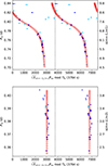 |
Fig. B.1. Stretched period échelle diagram of ℓ = 1 (top) and ℓ = 2 (bottom) mode frequencies. Navy blue dots: observed frequencies used for the analysis. Light blue dots: observed frequencies that are possible frequency combinations and not used for the analysis. Red circles: best-model frequencies. The size of the dots is proportional to the mode amplitude. |
Prior distributions for the dip model.
Estimated seismic parameters for the dip model.
Appendix C: Structure model of KIC 2309579
We computed for our study structure models calibrated on KIC 2309579. We calibrated the model with its buoyancy radius (Π0 = 3880 ± 100s). We used measurements reported in the Gaia DR3 (Gaia Collaboration 2023) for its effective temperature (Teff = 6938 ± 38K), it surface metallicity ((Z/X)s = 0.0108 ± 0.0035) and its bolometric luminosity. For the latter, we find two significantly different values in the Gaia DR3: the GSP-Phot luminosity L/L⊙ = 10.49 ± 0.90 and the FLAME luminosity L/L⊙ = 8.68 ± 0.25. We thus made models calibrated with this two values.
Models have been computed using the CESAM2k20 code (Morel 1997; Morel & Lebreton 2008; Manchon et al. 2025) and the Optimal Stellar Models (OSM) package. Mass and age are free parameters (mainly constrained by Teff and L). We adopted a solar metal mixture (Asplund et al. 2009) with meteoritic abundances for refractory elements from Serenelli (2010). The initial metallicity (Z/X)i is a free parameter (mainly constrained by (Z/X)s), and we considered three values for the initial helium abundance Yi = 0.25, 0.26 and 0.27. We used opacity tables from OPAL, the OPAL2005 equation of state (Rogers & Nayfonov 2002) and the nuclear reaction rates from the NACRE collaboration (Angulo et al. 1999) except for the  reaction, for which we used the LUNA reaction rate given in Imbriani et al. (2004). Convection was treated using the mixing-length theory (Böhm-Vitense 1958) with a mixing-length parameter αMLT = 1.77, close to a solar calibration, αMLT = 1.0, or αMLT = 0.5. Models include the effect of atomic diffusion following the Michaud & Proffitt (1993) formalism with radiative acceleration of Alecian & LeBlanc (2020). We adopted the Montreal prescription (Richer et al. 2000) for turbulent diffusion, calibrated with the parameterization of Verma & Silva Aguirre (2019). Models include also overshooting of the convective core with three prescriptions: (i) diffusive overshoot, (ii) instant mixing overshoot, (iii) instant mixing overshoot with adiabatic extension of the core. The overshoot parameter is free, mainly calibrated to reproduce Π0. The overshoot needed to reproduce Π0 is typically 0.23 ∼ 0.29Hp for instant mixing or 0.024 ∼ 0.028 for diffusive mixing. These values are consistent with the study of Mombarg et al. (2021). We also computed a fourth series of models with a fixed overshoot of 0.1Hp, but with a free extra uniform turbulent diffusion in the radiative zone, to build models similar to the γ Dor models of Ouazzani et al. (2020). We need a diffusion coefficient Dt = 600 ∼ 750 cm2 s−1 to fit the observations. Here we used different overshoot or turbulent mixing prescriptions to mimic any mixing processes that would impact these layers (for example, rotational mixing).
We ended up with 72 models with masses from 1.36 to 1.56 M⊙ with central hydrogen ranging between 0.25 and 0.38, that is between one half and two third of the central hydrogen reservoir has been burned. We used these different models to explore the influence of modeling uncertainties on the magnetic field strength determination. The value of Yi has almost no impact, αMLT has a strong impact on the upper layers, the amplitude of Kr(r) below the convective zone and the value of ℐ, but finally no impact on the measured value of magnetic field above the core. The overshoot and mixing prescription changes the shape of the Brunt-Väisälä frequency above the convective core and thus the detailed shape of Kr(r), but it only weakly affects the estimated magnetic field strength in this region.
Figure C.2 displays the critical magnetic field profile Bc in a model of KIC 2309579 computed for the lowest ℓ = 1 mode frequency (f66). We verify that, near the core, the magnetic field measured in KIC 2309579 (about 4 kG) is lower than Bc. As Bc increases with the frequency, the measured field remains lower than Bc for all the observed modes. We performed this computation with our 72 models and verified that a field Br ≈ 4 kG remains below Bc for all of them.
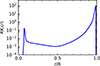 |
Fig. C.1. Magnetic weight function Kr(r) adimensionalized by the stellar radius R as a function of the normalized radius r, computed for a model of KIC 2309579. |
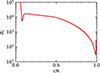 |
Fig. C.2. Critical magnetic field as a function of the radius, plotted for a representative model of KIC 2309579 with Yi = 0.26, a diffusive overshoot and calibrated of the GSP-Phot luminosity (see text). |
Appendix D: Extracted frequencies of KIC 2309579
We performed the analysis of the light curve of KIC 2309579 with a prewhitening technique using the FELIX code (Charpinet et al. 2010; Zong et al. 2016). We extracted frequencies with a signal-to-noise ratio greater than 4.7, that is a 4σ detection level. Figure D.1 displays the oscillation spectrum of KIC 2309579. Table D.1 lists the extracted frequencies along with their errors, amplitudes, and signal-to-noise ratios. Since linear combinations and/or harmonics could arise, we specify the possible linear combinations within 2σ error bars. We clearly identified ℓ = 1 and ℓ = 2 Kelvin modes as groups of peaks around 15 and 30μHz. We also identify a peak around 11.50μHz as the surface rotation νrot, as well as its harmonics at 2, 3, 4νrot. During the prewhitening process, the rotation peak has been fitted with two very close large peaks, f01 and f02, with different phases, presumably to take into account a modulation of its amplitude, which could be due to the finite lifetime of surface spots, latitudinal differential rotation, or even time variations of surface chemical inhomogeneities. Near the rotation frequency, there are a few frequencies that could be identified as Rossby modes and would require a dedicated analysis.
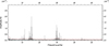 |
Fig. D.1. Oscillation spectrum of KIC 2309579. The frequency axis is represented in μHz, and the amplitude axis is represented in %. The dashed red curve represents the 4σ noise threshold before prewhitening. |
Extracted frequencies of KIC 2309579.
For the frequencies that have been modeled during the analysis, Table D.1 shows their associated degree ℓ and azimuthal order m. We also carried out an a posteriori identification of their radial orders n considering the optimal parameters of our model. Frequencies that could be linear combinations within a 2σ error bar but are well represented by our best-model are noted with a question mark next to their radial orders.
All Tables
All Figures
|
Fig. 1. Dimensionless seismic variable δKa as a function of the spin parameter sn, 1 for the 155 γ Dor stars from the Li et al. (2020) catalog. A dashed black curve shows the asymptotic approximation δKTh (see Lignières et al. 2024). Colors indicate the stellar rotation rate. |
| In the text | |
|
Fig. 2. Dimensionless seismic variable δKa as a function of the spin parameter sn, 1 for modes identified in KIC 2309579. For comparison, we plot the median δKa of the 155 stars (blue line) and the asymptotic approximation δKTh (orange dashes). |
| In the text | |
|
Fig. 3. Stretched period échelle diagram of ℓ = 1 (top) and ℓ = 2 (bottom) Kelvin mode frequencies. Navy blue dots indicate observed frequencies used for the analysis. Light blue dots represent observed frequencies that are possible frequency combinations and discarded for the analysis. Red circles are frequencies of the best model including a magnetic field. The size of the dots is proportional to the mode amplitude. |
| In the text | |
|
Fig. B.1. Stretched period échelle diagram of ℓ = 1 (top) and ℓ = 2 (bottom) mode frequencies. Navy blue dots: observed frequencies used for the analysis. Light blue dots: observed frequencies that are possible frequency combinations and not used for the analysis. Red circles: best-model frequencies. The size of the dots is proportional to the mode amplitude. |
| In the text | |
|
Fig. C.1. Magnetic weight function Kr(r) adimensionalized by the stellar radius R as a function of the normalized radius r, computed for a model of KIC 2309579. |
| In the text | |
|
Fig. C.2. Critical magnetic field as a function of the radius, plotted for a representative model of KIC 2309579 with Yi = 0.26, a diffusive overshoot and calibrated of the GSP-Phot luminosity (see text). |
| In the text | |
|
Fig. D.1. Oscillation spectrum of KIC 2309579. The frequency axis is represented in μHz, and the amplitude axis is represented in %. The dashed red curve represents the 4σ noise threshold before prewhitening. |
| In the text | |
Current usage metrics show cumulative count of Article Views (full-text article views including HTML views, PDF and ePub downloads, according to the available data) and Abstracts Views on Vision4Press platform.
Data correspond to usage on the plateform after 2015. The current usage metrics is available 48-96 hours after online publication and is updated daily on week days.
Initial download of the metrics may take a while.