| Issue |
A&A
Volume 710, June 2026
|
|
|---|---|---|
| Article Number | L16 | |
| Number of page(s) | 6 | |
| Section | Letters to the Editor | |
| DOI | https://doi.org/10.1051/0004-6361/202660616 | |
| Published online | 12 June 2026 | |
Letter to the Editor
Towards inertial-mode helioseismology: Direct sensing of solar rotation at 75° latitude and 0.8 R⊙
1
Max-Planck-Institut für Sonnensystemforschung, Justus-von-Liebig-Weg 3, 37077 Göttingen, Germany
2
Institut für Astrophysik und Geophysik, Georg-August-Universtät Göttingen, Friedrich-Hund-Platz 1, 37077 Göttingen, Germany
3
Center for Astrophysics and Space Science, NYUAD Institute, New York University Abu Dhabi, Abu Dhabi, United Arab Emirates
★ Corresponding author: This email address is being protected from spambots. You need JavaScript enabled to view it.
Received:
25
April
2026
Accepted:
6
May
2026
Abstract
Context. Because solar global inertial modes are highly sensitive to differential rotation, they may provide new diagnostics of internal rotation at high latitudes, where acoustic-mode helioseismology provides only weak constraints.
Aims. Our aim was to constrain solar rotation using the measured frequency of the m = 1 high-latitude inertial mode, starting from the HMI/SDO reference rotation profile given by p-mode helioseismology for 2010–2024.
Methods. Using a validated and accurate eigenvalue solver, we computed the perturbation to the mode frequency resulting from localized changes in the differential rotation rate throughout the solar interior.
Results. We find that the linear sensitivity kernel of the m = 1 high-latitude mode peaks at a latitude of 75° and a radius of 0.8 R⊙, with full widths of 7° and 0.13 R⊙. From the observed mode frequency in the Carrington frame, −87.9 ± 1.9 nHz (retrograde, averaged over 2010–2024), we infer that the solar rotation rate near this location is 365.3 ± 2.0 nHz, which exceeds the reference p-mode estimate by 8.1 nHz. Additionally, we propose a latitudinally smooth, radially independent modification to the rotation rate at high latitudes beyond the linear (small-perturbation) regime.
Conclusions. This work demonstrates that individual inertial modes can provide direct constraints on rotation in the bulk of the solar convection zone, well below the surface, representing the first example of spatially resolved inertial-mode helioseismology.
Key words: hydrodynamics / Sun: helioseismology / Sun: interior / Sun: oscillations / Sun: rotation
© The Authors 2026
 Open Access article, published by EDP Sciences, under the terms of the Creative Commons Attribution License (https://creativecommons.org/licenses/by/4.0), which permits unrestricted use, distribution, and reproduction in any medium, provided the original work is properly cited.
This article is published in open access under the Subscribe to Open model.
Open access funding provided by Max Planck Society.
1. Introduction
Internal differential rotation is crucial for understanding the Sun’s dynamo and angular momentum transport mechanisms (e.g., Käpylä et al. 2023). Our current knowledge of the Sun’s differential rotation comes primarily from p-mode helioseismology, which exploits the frequency splittings of modes with different azimuthal orders (e.g., Thompson et al. 2003). The Sun’s convection zone (CZ), which constitutes the outer 30% of the Sun, rotates differentially, varying with both radius and latitude, while the radiative interior rotates almost rigidly. The tachocline exists at the transition between these two zones (e.g., Spiegel & Zahn 1992), and there is also a near-surface shear layer in the outermost 5% of the solar radius (e.g., Thompson et al. 1996).
Despite remarkable achievements, p-mode helioseismology still faces significant limitations. It provides limited information about the Sun’s rotation below ∼0.2 R⊙ (e.g., Gizon et al. 1997) and in regions within ∼20° of the rotation axis (e.g., Schou et al. 1998). This limitation arises because very few p-modes have appreciable kinetic energy density in these regions, as their sensitivity kernels peak near the solar surface. As a consequence, inversions of frequency splittings obtained using various methods can differ significantly in the polar regions (Thompson et al. 2003, their Figure 7).
Solar inertial modes are low-frequency global modes of oscillation that are restored by the Coriolis force. These are retrograde modes with a strong toroidal component and periods on timescales comparable to the solar rotation period (∼25 days at the equator). Maps of horizontal flows near the solar surface have been measured for more than a decade using p-mode local helioseismology and local correlation tracking applied to data from the Helioseismic and Magnetic Imager aboard the Solar Dynamics Observatory (HMI/SDO) and Global Oscillations Network Group (GONG). These long-duration observations allow for the unambiguous detection and characterization of solar inertial modes (Löptien et al. 2018; Gizon et al. 2021; Hanson et al. 2022).
In this work we focus on the high-latitude mode with azimuthal wavenumber m = 1 and north-south symmetric radial vorticity (hereafter the HL1 mode). This mode has been observed to have the largest amplitude on the surface of the Sun, in the range 5–25 m/s at latitudes above 60° (Gizon et al. 2021). It has been consistently detected in multiple datasets and is also present in the Mount Wilson Observatory Dopplergrams spanning the last five sunspot cycles (Ulrich 2001; Liang & Gizon 2025). The frequency of the HL1 mode is known to a high degree of precision. Over the period of HMI observations, its mean frequency in the Carrington frame is ωobs/2π = −87.9 ± 1.9 nHz (Fig. 1).
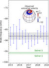 |
Fig. 1. Observed HL1 frequencies in the Carrington reference frame extracted from HMI Dopplergrams at a cadence of one year with a three-year sliding window (blue points with error bars, Liang & Gizon 2025). The mean frequency ωobs/2π = −87.9 nHz is indicated by the black horizontal line, and the gray shaded region shows the ±1σ range (±1.9 nHz). The frequency uncertainty was estimated from measurements over independent time intervals centered on 2012, 2015, 2018, and 2021, thereby accounting for correlations introduced by the sliding window. The solid green line marks the real part of the eigenfrequency computed using eigenvalue Solver 1 (−95.6 nHz), and the dashed green line marks the same for Solver 2 (−96.1 nHz). The azimuthal velocity of the observed mode at the surface is shown as an inset (adapted from Gizon et al. 2021). |
Because their physics is intrinsically linked to rotation, inertial modes are particularly well suited for diagnosing differential rotation (see Goddard et al. 2020, for the case of Rossby modes). Linear eigenmode computations have indicated that the kinetic energy density of the HL1 mode peaks inside the convection zone (Gizon et al. 2021; Bekki et al. 2022), making it a very promising candidate for directly probing rotation in the solar interior.
2. Mismatch between model and observed frequencies of HL1 inertial mode
In order to place constraints on the solar internal rotation using the observed frequency of the HL1 mode, we needed to solve the forward problem, that is, to compute the mode frequency for a given prescription of the solar differential rotation (see Appendix A). We denoted the solar angular velocity measured in an inertial frame by Ω(r, θ), where r is the radius and θ is the colatitude (θ = 0 at the north pole). We adopted the reference differential rotation rate Ωref(r, θ) derived from p-mode helioseismology (Larson & Schou 2018). In the Carrington frame rotating at angular frequency ΩCarr/2π = 456.0 nHz, we linearized the equations of momentum, entropy, and continuity about a standard solar model (Model S, Christensen-Dalsgaard et al. 1996). The computational domain extends radially over the range 0.65 R⊙ < r < 0.985 R⊙. We assumed perturbations proportional to exp(imϕ − iωt), where m = 1 and ϕ is the longitude. Under horizontal stress-free boundary conditions, the system yields a discrete spectrum of complex eigenvalues ω and corresponding eigenvectors. We used an eigenvalue solver based on Bekki et al. (2022) to compute the eigenmodes in the inertial frequency range (Solver 1; see Appendix A). This solver was validated through a code-to-code benchmark comparison with the independent implementation of Mukhopadhyay et al. (2025) (Solver 2; see Appendix A). The m = 1 high-latitude eigenmode is identified in the spectrum as the only self-excited low-frequency mode (ℑω > 0) that exhibits north-south symmetric radial vorticity. Using Solver 1, we obtained a model eigenfrequency of ωref/2π = −95.6 + 3.9 i nHz in the Carrington frame. The real part of ωref thus differs from the observed ωobs by four standard deviations (see Fig. 1). The velocity eigenfunction at the surface, however, is similar to the observation, with power confined to a similar latitudinal range above 60° and a qualitatively similar spiral pattern.
We performed a set of eigenvalue computations that indicate that this discrepancy is likely due to an incorrect reference differential rotation profile. This discrepancy cannot be fixed by varying the other parameters of the background solar model, such as the viscous or thermal diffusivities or the superadiabaticity. In particular, we computed eigenmodes around the commonly used value of turbulent diffusivity in the convection zone νCZ = 1012 cm2 s−1. Within the range 1011 cm2 s−1 ≤ νCZ ≤ 2 × 1012 cm2 s−1, we find that the eigenfrequency remains within the bounds 5.0 nHz < (ωobs − ℜω)/2π < 10.0 nHz, indicating that the diffusion cannot be used as a tunable parameter to bring the eigenfrequency within observational errorbars. Further, we find that the superadiabaticity (δ = ∇ − ∇ad) affects the eigenfrequency only weakly, by at most 3 nHz when the superadiabatic gradient is varied in the range |δ|< 5 × 10⁻⁷. This motivates focusing on the background rotation rate as the primary physical parameter of the model that can be adjusted to bring the model into agreement with the observations, while keeping δ = 0 and νCZ = 1012 cm2 s−1 fixed.
3. Sensitivity of HL1 mode frequency to the local rotation rate
The linear sensitivity of the mode frequency to a spatial change in rotation is specified through the integral equation
 (1)
(1)
where δω = ω − ωref is the perturbation to the (complex) eigenfrequency that results from a small perturbation in the rotation rate, δΩ = Ω − Ωref, and K is the (complex) sensitivity kernel. The discretized version of this equation is
 (2)
(2)
where dΣ = r dr dθ is the surface element in the meridional plane (expressed in terms of the radial and latitudinal grid spacings, dr = 2.3 Mm and dθ = 2.0°) used in our calculations. The most straightforward method for computing the sensitivity kernel is numerical. For a given spatial pixel (ri, θj) where the kernel is to be evaluated, we considered a rotation profile that is perturbed only at that pixel,
 (3)
(3)
where the grid (rp, θq) spans the full numerical domain. Here, δpi and δqj are Kronecker delta functions. The perturbation amplitude ϵ must be sufficiently small to ensure that the resulting change in oscillation frequency remains in the linear regime. We chose ϵ/2π = 1.0 nHz. The latitudinal entropy gradient was also perturbed numerically to maintain thermal wind balance. Using Solver 1, we computed the eigenfrequency of the high-latitude mode, ωϵ(ri, θj), for this perturbed system. The sensitivity kernel at pixel (i, j) was then given by
![Mathematical equation: $$ \begin{aligned} K(r_i, \theta _j)\ \mathrm{d}\Sigma =[{\omega _\epsilon (r_i,\theta _j)-\omega _{\rm ref}}]/{\epsilon }. \end{aligned} $$](/articles/aa/full_html/2026/06/aa60616-26/aa60616-26-eq4.gif) (4)
(4)
The real part of the kernel, presented in Fig. 2, shows a prominent peak centered at (r0, θ0) = (0.82 R⊙, 15° ) and two smaller sidelobes, one positive and one negative, at 0.72 R⊙. The main peak of the kernel has full widths at half maximum of 7° in latitude and 0.13 R⊙ in radius, as shown in the cuts in Figs. B.1 and B.2. We found almost no sensitivity in the radiative interior.
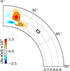 |
Fig. 2. Spatial sensitivity of the frequency of the HL1 mode to localized changes in the background rotation rate. The kernel K(r, θ) is symmetric across the equator. Grid sizes dr = 2.3 Mm and dθ = 2° were used for this calculation. For reference, a patch of area 10dr × 2rdθ = 20dΣ is outlined with a solid black contour. The dashed black contour corresponds to the value of the kernel at half maximum. |
Because the kernel is reasonably well localized in both radius and latitude, the inferred frequency shift can be interpreted as providing a direct estimate of the local rotation perturbation at location (r0, θ0). Specifically, the observed frequency difference can be related to the local change in rotation rate through the integral of the kernel over the meridional plane. The total integral of the kernel over the meridional plane, ∑ijK(ri, θj)dΣ = 0.95 + 0.03 i, has a real part that is close to unity1. We did not attempt a quantitative interpretation of the imaginary part since there is presently no established method to relate the imaginary part of the mode frequency to an observable (such as the mode amplitude, see Mushtaq et al. 2026, for a preliminary weakly nonlinear approach in 2D). Using the constraint (ωobs − ℜωref)/2π = 7.7 ± 1.9 nHz, we estimated the perturbation to the rotation rate near (r0, θ0) as
 (5)
(5)
This small but significant enhancement of the rotation rate relative to the p-mode reference value (Ωref(r0, θ0)/2π = 357.2 nHz) shows that the HL1 mode provides a sensitive probe of differential rotation at high latitudes in the deep convection zone.
The above constraint is compared in Fig. 4 with a p-mode rotation estimate at (r0, θ0) obtained using optimally localized averaging (OLA; Howe 2009). This method combines p-mode frequency splittings to produce a resolution kernel localized at the target position (Pijpers & Thompson 1992, 1994). A significant discrepancy can be observed at a colatitude where OLA inversions are most uncertain. Remarkably, a single inertial mode yields a kernel with a comparable latitudinal extent.
4. Parametric model for rotation correction
To study the effect of a smooth modification to the rotation rate at high latitudes, we defined a simple parametric correction that depends only on the colatitude:
![Mathematical equation: $$ \begin{aligned} \Delta \Omega (\theta ; A) = {\left\{ \begin{array}{ll} A&\theta < 10^\circ , \\ A [1 + \sin \left( 4.5 (30^\circ -\theta )\right) ]/2&10^\circ \le \theta < 50^\circ , \\ 0&50^\circ \le \theta < 90^\circ . \end{array}\right.} \end{aligned} $$](/articles/aa/full_html/2026/06/aa60616-26/aa60616-26-eq6.gif) (6)
(6)
This rotation perturbation is symmetric across the equator. In the above equation, the profile reaches a maximum amplitude (A) at the pole and has a width of 30° (see Fig. 3a). This perturbation is radially constant, and it therefore also affects the rotation rate in the radiative zone. However, we showed in the previous section that the mode is insensitive to rotation in the radiative zone, and we chose not to include radial dependence of the profile for simplicity.
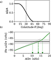 |
Fig. 3. Smooth high-latitude modification to the background rotation rate, ΔΩ(θ; A), and its effect on the HL1 mode frequency. (a) Functional form of ΔΩ(θ; A) as defined by Eq. (6), symmetric across the equator. (b) Variation of the real part of the mode frequency with A when using Solver 1 (green curve). By construction ω = ωref at A = 0. Agreement with the observed eigenfrequency (gray shaded region) is obtained for 10.3 nHz < A/2π < 16.0 nHz (range between the dotted green arrows). The value of A/2π = 13.6 nHz corresponding to the best fit is marked by the dashed green arrow. The dotted black line shows the linear approximation Eq. (7). |
For infinitesimal perturbations in the angular velocity parameterized as above (i.e., as A → 0), the response of the mode frequency is
 (7)
(7)
In the linear regime, A ≈ (ωobs − ℜωref)/0.65. However, the range of validity of this linear approximation is not yet established, motivating the direct numerical computations of ℜδω(A) for finite-amplitude values of A.
We recomputed the eigenfrequency of the mode with the modified rotation rate Ω(r, θ) = Ωref(r, θ)+ΔΩ(θ; A) for values of A/2π ranging from 0 to 20 nHz. In all cases, the latitudinal entropy gradient was recomputed such that the thermal wind balance is maintained. The variation of the real part of the eigenfrequency with A is presented in Fig. 3b. The relationship between the real part of the eigenfrequency and A is roughly linear for A/2π ≲ 16 nHz. For A/2π between 10.3 nHz and 16.0 nHz, the real part of the eigenfrequency is within ±1σ of the observed frequency and the imaginary part of the frequency is positive (the mode is linearly unstable). A profile of the modified rotation rate at r = 0.8 R⊙ is shown in Fig. 4 for  nHz, giving a polar rotation rate of 364.0 nHz.
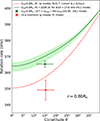 |
Fig. 4. Constraints on high-latitude solar rotation rate at r = 0.8 R⊙. The green cross shows the constraint from the HL1 mode frequency (2010–2024), according to Eq. (5), with the horizontal bar indicating the width of the kernel. The green curve shows the rotation rate Ωref(r, θ)+ΔΩ(θ; A) for A/2π = 13.6 nHz, and the green shaded region indicates the associated uncertainty (see Fig. 3). The p-mode reference rotation rate Ωref(0.8 R⊙, θ) is given by the red dashed curve. The red cross shows a p-mode OLA estimate at the target location (0.8 R⊙, θ = 15° ) obtained from yearly HMI inversions (Howe 2009) averaged over 2010–2023. The horizontal bar represents the width of the averaging kernel, while the vertical bar represents the random error. |
5. Conclusion
We find that the rotation kernel of the HL1 mode frequency is highly localized in the convection zone near r = 0.8 R⊙ and θ = 15°. Without performing any inversion, the integrated HL1 kernel implies a local rotation rate of approximately 365.3 ± 2.0 nHz at this location, that is, 8.1 ± 2.0 nHz above the reference estimate from p-mode helioseismology (Larson & Schou 2018) and above a p-mode OLA inversion (Howe 2009). Using the smooth parametric profile prescribed in Sect. 4, the inferred enhancement reaches 13.6 ± 3 nHz at the pole relative to the reference model. These estimates are absolute measurements in the sense that we used the frequency of a single retrograde inertial mode. In contrast, acoustic modes infer the rotation rate using a differential measurement between prograde and retrograde modes, which reduces dependencies on the background model.
The frequencies of many other solar inertial modes have been measured (Gizon et al. 2021), as well as their variations with the solar cycle (Waidele & Zhao 2023; Lekshmi et al. 2026). In future work, we will aim to constrain the solar differential rotation at multiple positions in the convection zone using all modes simultaneously by solving an inverse problem. In this respect, the current situation is reminiscent of the early days of helioseismology, when Christensen-Dalsgaard & Gough (1976) foresaw the potential of p modes as probes of the solar interior. The validated eigenvalue solvers described in this paper will be valuable tools in this respect, particularly for interpreting the full spectrum of inertial modes and for assessing the contribution of time-varying zonal flows to their temporal variations (see Goddard et al. 2020).
Acknowledgments
PD and LG designed and performed research, PD and YB updated an earlier version of Solver 1, PD wrote the first draft of the paper and all authors contributed to the final manuscript. The authors acknowledge the essential contribution of Suprabha Mukhopadhyay, which enabled the cross-validation of Solver 1 with Solver 2. We thank Zhi-Chao Liang for making available the HL1 mode frequencies shown in Fig. 1 and Rachel Howe for providing the p-mode OLA rotation inversion shown in Fig. 4. We acknowledge useful discussions with Damien Fournier and Robert Cameron. We acknowledge partial financial support from ERC Synergy Grant WHOLESUN (grant agreement No. 810218) to LG. PD is a member of the International Max Planck Research School for Solar System Science at the University of Göttingen.
References
- Bekki, Y., Cameron, R. H., & Gizon, L. 2022, A&A, 662, A16 [NASA ADS] [CrossRef] [EDP Sciences] [Google Scholar]
- Burns, K. J., Vasil, G. M., Oishi, J. S., Lecoanet, D., & Brown, B. P. 2020, Phys. Rev. Res., 2, 023068 [NASA ADS] [CrossRef] [Google Scholar]
- Christensen-Dalsgaard, J., & Gough, D. O. 1976, Nature, 259, 89 [NASA ADS] [CrossRef] [Google Scholar]
- Christensen-Dalsgaard, J., Dappen, W., Ajukov, S. V., et al. 1996, Science, 272, 1286 [Google Scholar]
- Fan, Y., & Fang, F. 2014, ApJ, 789, 35 [NASA ADS] [CrossRef] [Google Scholar]
- Gizon, L., Fossat, E., Lazrek, M., et al. 1997, A&A, 317, L71 [Google Scholar]
- Gizon, L., Cameron, R. H., Bekki, Y., et al. 2021, A&A, 652, L6 [NASA ADS] [CrossRef] [EDP Sciences] [Google Scholar]
- Goddard, C. R., Birch, A. C., Fournier, D., & Gizon, L. 2020, A&A, 640, L10 [NASA ADS] [CrossRef] [EDP Sciences] [Google Scholar]
- Hanson, C. S., Hanasoge, S., & Sreenivasan, K. R. 2022, Nat. Astron., 6, 708 [NASA ADS] [CrossRef] [Google Scholar]
- Howe, R. 2009, Liv. Rev. Sol. Phys., 6, 1 [Google Scholar]
- Käpylä, P. J., Browning, M. K., Brun, A. S., Guerrero, G., & Warnecke, J. 2023, Space Sci. Rev., 219, 58 [CrossRef] [Google Scholar]
- Larson, T. P., & Schou, J. 2018, Sol. Phys., 293, 29 [Google Scholar]
- Lehoucq, R., Sorensen, D., & Yang, C. 1998, ARPACK Users’ Guide: Solution of Large-scale Eigenvalue Problems with Implicitly Restarted Arnoldi Methods (Philadelphia: SIAM) [Google Scholar]
- Lekshmi, B., Liang, Z. C., Gizon, L., Philidet, J., & Jain, K. 2026, A&A, submitted [arXiv:2602.03741] [Google Scholar]
- Liang, Z.-C., & Gizon, L. 2025, A&A, 695, A67 [NASA ADS] [CrossRef] [EDP Sciences] [Google Scholar]
- Löptien, B., Gizon, L., Birch, A. C., et al. 2018, Nat. Astron., 2, 568 [Google Scholar]
- Mukhopadhyay, S., Bekki, Y., Zhu, X., & Gizon, L. 2025, A&A, 696, A160 [NASA ADS] [CrossRef] [EDP Sciences] [Google Scholar]
- Mushtaq, M., Fournier, D., Ayoub, R., Schmid, P. J., & Gizon, L. 2026, A&A, submitted [arXiv:2603.08528] [Google Scholar]
- Pijpers, F. P., & Thompson, M. J. 1992, A&A, 262, L33 [NASA ADS] [Google Scholar]
- Pijpers, F. P., & Thompson, M. J. 1994, A&A, 281, 231 [NASA ADS] [Google Scholar]
- Rempel, M. 2005, ApJ, 622, 1320 [NASA ADS] [CrossRef] [Google Scholar]
- Schou, J., Antia, H. M., Basu, S., et al. 1998, ApJ, 505, 390 [Google Scholar]
- Spiegel, E. A., & Zahn, J. P. 1992, A&A, 265, 106 [NASA ADS] [Google Scholar]
- Thompson, M. J., Toomre, J., Anderson, E. R., et al. 1996, Science, 272, 1300 [Google Scholar]
- Thompson, M. J., Christensen-Dalsgaard, J., Miesch, M. S., & Toomre, J. 2003, ARA&A, 41, 599 [Google Scholar]
- Ulrich, R. K. 2001, ApJ, 560, 466 [CrossRef] [Google Scholar]
- Waidele, M., & Zhao, J. 2023, ApJ, 954, L26 [NASA ADS] [CrossRef] [Google Scholar]
The total integral of the kernel can also be computed directly by perturbing the reference rotation rate by a constant value ϵ; this yields δω/ϵ = 0.96 + 0.03 i, confirming the accuracy of the eigenvalue solver.
Appendix A: Computation of eigenmodes of a rotating solar model
A.1. Linearized equations of motion
We work in the Carrington frame of reference, rotating at frequency ΩCarr/2π = 456.0 nHz with respect to an inertial frame. We use the linearized forms of the momentum, entropy, and continuity equations, where perturbations in velocity (v′), pressure (p′), density (ρ′), and entropy (s′) are proportional to exp[i(mϕ − ωt)], where ϕ is the longitude and ω is the angular frequency of the mode of oscillation, to obtain
 (A.1)
(A.1)
 (A.2)
(A.2)
 (A.3)
(A.3)
In the above equations, the unprimed variables (ρ, p, g, s, T) refer to the background reference state, and κ is the thermal diffusivity. The unit vectors  ,
,  , and
, and  point in the radial, longitudinal, and rotation-axis directions, respectively. An ideal gas equation of state is used to close the equations. The perturbations are complex functions of radius and colatitude. The components of the viscous stress tensor 𝒟 are given by
 (A.4)
(A.4)
where the Sij are the components of the deformation tensor in spherical coordinates (Fan & Fang 2014) and νturb is the turbulent viscosity.
A.2. Boundary conditions
Complemented by boundary conditions, the above equations constitute an eigenvalue problem. We choose the computational domain to span 0.65 R⊙ to 0.985 R⊙ in radius. We use impenetrable horizontal stress-free boundary conditions for the velocity at the top and bottom boundaries, and assume there is no entropy flux at either boundary:
 (A.5)
(A.5)
Further, we assume the perturbations vr′, vϕ′, ρ′, and s′ to vanish at the poles (θ = 0 and π). For the specific case of m = 1 (our case), we require ∂vθ′/∂θ = 0. This allows for a polar crossing flow. With these boundary conditions, Eqs. (A.1)–(A.3) form an eigenvalue problem, which is non-singular because of the viscous stresses Eq. (A.4). The spectrum of eigenvalues ω is discrete.
A.3. Reference solar model and reference differential rotation
We use the background density, pressure, and gravitational acceleration from the standard solar model S (Christensen-Dalsgaard et al. 1996). The reference internal rotation is provided by p-mode helioseismology (Larson & Schou 2018) applied to data from HMI/SDO. The time series of the angular velocity Ω(r, θ; t) is derived from successive data segments of length 72 days and 36 a-coefficients, a standard product available for download at the Joint Science Operations Center (JSOC) website under the filename hmi.v_sht_2drls. We adopt as the background rotation rate the mean profile from 30 April 2010 to 16 February 2024 and denote it by Ωref(r, θ), see Fig. A.1.
 |
Fig. A.1. The reference solar angular velocity in the Carrington frame, Ωref − ΩCarr, from p-mode helioseismology (Larson & Schou 2018). This meridional cut shows the computational domain for the eigenvalue solvers, 0.65 < r/R⊙ < 0.985. |
We need to specify ∇s in Eq. (A.2). Invoking the thermal wind balance for the latitudinal derivative of the entropy (Rempel 2005), we obtain
 (A.6)
(A.6)
where cp is the specific heat at constant pressure, Hp is the pressure scale height, and δ = ∇ − ∇ad is the superadiabatic temperature gradient. Because the convection zone is nearly adiabatically stratified, we set δ = 0 there and smoothly transition in the radiative interior (r/R⊙ < 0.70) to the value of δ(r) from Model S.
We also need to specify νturb in Eq. (A.4). We adopt a turbulent viscosity profile in the form of a step function:
![Mathematical equation: $$ \begin{aligned} \nu _{\rm turb}(r) =\nu _{\rm RZ}+\frac{\nu _{\rm CZ}-\nu _{\rm RZ}}{2}\left[1+\tanh (\frac{r/R_\odot - 0.7}{0.015})\right], \end{aligned} $$](/articles/aa/full_html/2026/06/aa60616-26/aa60616-26-eq18.gif) (A.7)
(A.7)
where νRZ = 109 cm2 s−1 and νCZ = 1012 cm2 s−1 are representative values of the turbulent viscosities in the radiative and convection zones. We use the same profile for the thermal diffusivity.
A.4. Two eigenvalue solvers
Numerical eigenmodes may depend on the computational methods and codes. Therefore, we considered two independent codes, which use different discretization methods to solve the same problem. The first eigenvalue solver, referred to as ‘Solver 1’, is based on the finite-difference solver of Bekki et al. (2022). The second solver, ‘Solver 2’, is the Dedalus-based spectral solver described by Mukhopadhyay et al. (2025). Resolution-based convergence tests were performed to ensure numerical accuracy.
A.5. Solver 1 based on Bekki et al. (2022)
Solver 1 uses a uniform (staggered) grid in radius and colatitude, and a second-order finite difference scheme to compute derivatives. We use 100 radial and 90 latitudinal gridpoints, corresponding to resolutions of 2.3 Mm and 2°. The details of the grid and the computation methods was presented originally in Bekki et al. (2022). During validation, we found a number of bugs in the code, related to the treatment of the viscous and thermal diffusivities. We use a revised version of the code, where these bugs are corrected for. In addition, we upgraded the Fortran eigenvalue solver from the LAPACK package to ARPACK (a sparse solver, see Lehoucq et al. 1998) to speed up the computations.
At fixed m = 1, we compute the 100 eigenfrequencies nearest to the (real) target frequency of −90 nHz in the Carrington frame. We identify the mode with the largest growth rate (largest imaginary part of the eigenvalue) as the mode of interest. This mode has north-south symmetric radial vorticity, as observed on the Sun. Solver 1 gives a mode frequency of ℜωref/2π = −95.6 nHz in the Carrington frame (see solid green line in Fig. 1). This is also the only self-excited mode with symmetric radial vorticity in the computed eigenspectrum.
A.6. Solver 2 from Mukhopadhyay et al. (2025)
Dedalus (Burns et al. 2020) is an open-source, parallel code that solves partial differential equations in spectral space. It uses Chebyshev polynomials and spherical harmonics as radial and horizontal basis functions respectively to compute the eigenvalues of a system. Previously, Mukhopadhyay et al. (2025) used Dedalus to develop an eigenvalue solver for solar inertial modes (hereafter Solver 2). To validate Solver 1, we used Solver 2 to compute the eigenmodes within the same computational domain. Solver 2 used 84 and 32 gridpoints in radius and colatitude respectively. We specify the same target frequency and compute the same number of eigenmodes as for Solver 1. The eigenmode with the largest growth rate has a real frequency of −96.1 nHz (see dashed line in Fig. 1) and a similar eigenfunction to that from Solver 1.
A.7. Importance of the position of the lower boundary
As part of our numerical investigations, we found that the inclusion of the upper radiative zone r = 0.65 R⊙ to 0.70 R⊙ in the computational domain plays an important role in unambiguously identifying the HL1 mode. When considering only the convection zone, as in Mukhopadhyay et al. (2025) or Bekki et al. (2022), the system produces two pairs of self-excited eigenmodes within ∼10 nHz; each pair consisting of two modes with opposite latitudinal symmetries in their eigenfunction. This is at odds with the observation of a single mode dominating the power spectrum. When the upper layers of the radiative zone are included in the model, however, we find only one pair of self-excited eigenmodes, with the fastest growing mode (eigenfrequency with the largest imaginary part) having the same north-south symmetry as that dominant in the observations. The surface profile of this mode is very similar to that extracted from surface observations.
Appendix B: Additional figures
All Figures
|
Fig. 1. Observed HL1 frequencies in the Carrington reference frame extracted from HMI Dopplergrams at a cadence of one year with a three-year sliding window (blue points with error bars, Liang & Gizon 2025). The mean frequency ωobs/2π = −87.9 nHz is indicated by the black horizontal line, and the gray shaded region shows the ±1σ range (±1.9 nHz). The frequency uncertainty was estimated from measurements over independent time intervals centered on 2012, 2015, 2018, and 2021, thereby accounting for correlations introduced by the sliding window. The solid green line marks the real part of the eigenfrequency computed using eigenvalue Solver 1 (−95.6 nHz), and the dashed green line marks the same for Solver 2 (−96.1 nHz). The azimuthal velocity of the observed mode at the surface is shown as an inset (adapted from Gizon et al. 2021). |
| In the text | |
|
Fig. 2. Spatial sensitivity of the frequency of the HL1 mode to localized changes in the background rotation rate. The kernel K(r, θ) is symmetric across the equator. Grid sizes dr = 2.3 Mm and dθ = 2° were used for this calculation. For reference, a patch of area 10dr × 2rdθ = 20dΣ is outlined with a solid black contour. The dashed black contour corresponds to the value of the kernel at half maximum. |
| In the text | |
|
Fig. 3. Smooth high-latitude modification to the background rotation rate, ΔΩ(θ; A), and its effect on the HL1 mode frequency. (a) Functional form of ΔΩ(θ; A) as defined by Eq. (6), symmetric across the equator. (b) Variation of the real part of the mode frequency with A when using Solver 1 (green curve). By construction ω = ωref at A = 0. Agreement with the observed eigenfrequency (gray shaded region) is obtained for 10.3 nHz < A/2π < 16.0 nHz (range between the dotted green arrows). The value of A/2π = 13.6 nHz corresponding to the best fit is marked by the dashed green arrow. The dotted black line shows the linear approximation Eq. (7). |
| In the text | |
|
Fig. 4. Constraints on high-latitude solar rotation rate at r = 0.8 R⊙. The green cross shows the constraint from the HL1 mode frequency (2010–2024), according to Eq. (5), with the horizontal bar indicating the width of the kernel. The green curve shows the rotation rate Ωref(r, θ)+ΔΩ(θ; A) for A/2π = 13.6 nHz, and the green shaded region indicates the associated uncertainty (see Fig. 3). The p-mode reference rotation rate Ωref(0.8 R⊙, θ) is given by the red dashed curve. The red cross shows a p-mode OLA estimate at the target location (0.8 R⊙, θ = 15° ) obtained from yearly HMI inversions (Howe 2009) averaged over 2010–2023. The horizontal bar represents the width of the averaging kernel, while the vertical bar represents the random error. |
| In the text | |
|
Fig. A.1. The reference solar angular velocity in the Carrington frame, Ωref − ΩCarr, from p-mode helioseismology (Larson & Schou 2018). This meridional cut shows the computational domain for the eigenvalue solvers, 0.65 < r/R⊙ < 0.985. |
| In the text | |
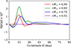 |
Fig. B.1. Cuts at different radii though the kernel presented in Fig. 2. |
| In the text | |
 |
Fig. B.2. Cuts at different latitudes of the kernel presented in Fig. 2. |
| In the text | |
Current usage metrics show cumulative count of Article Views (full-text article views including HTML views, PDF and ePub downloads, according to the available data) and Abstracts Views on Vision4Press platform.
Data correspond to usage on the plateform after 2015. The current usage metrics is available 48-96 hours after online publication and is updated daily on week days.
Initial download of the metrics may take a while.