| Issue |
A&A
Volume 546, October 2012
|
|
|---|---|---|
| Article Number | A2 | |
| Number of page(s) | 28 | |
| Section | Extragalactic astronomy | |
| DOI | https://doi.org/10.1051/0004-6361/201219578 | |
| Published online | 27 September 2012 | |
Online material
Appendix A: Catalogues of the H ii regions
 |
Fig. A.1
Left-panel: spatial distribution of the [O iii]/Hβ line ratio along the spatial extension of the UGC 1081 galaxy, derived from the analysis of the H ii regions. Each symbol corresponds to a H ii region, its filling colour corresponding to the shown parameter, scaled as displayed in the right-size colour-table. Red symbols correspond to H ii regions associated with arm 1, and black ones correspond to those associated with arm 2 (where the indexing of the arms was selected in arbitrary way). Grey symbols represent H ii regions without a clear association with a particular arm, following the criteria described in Sect. 5. The circles represent those H ii regions below the Kauffmann et al. (2003) demarcation line in the BPT diagram shown in Fig. 7, and the squares corresponds to those ones located in the intermediate region between that line and the Kewley et al. (2001) one. The size of the symbols are proportional to the Hα intensity. Right-panel: similar spatial distribution for the absolute value of the equivalent width of Hα in logarithm scale. Symbols are similar to those described for the left panel. |
| Open with DEXTER | |
The results of the overall analysis on the properties of the H ii regions is compiled in three different catalogues per galaxy, each of them comprising different information. The nomenclature of each catalogue is table.HII.TYPE.GALNAME.csv (for the coma separated version) or table.HII.TYPE.GALNAME.txt (for the space separated ones), where TYPE correspond to each of the following types: coords (coordinates of the H ii regions), flux (fluxes of the stronger emission lines) or EW (equivalent width of the stronger emission lines). GALNAME corresponds to the galaxy name as listed in Table 1.
The catalogues are stored in the CALIFA public ftp server:
ftp://ftp.caha.es/CALIFA/early_studies/HII/tables/ The content of each table is described in the following sections.
A.1. coords tables
They include all the information regarding the location of each H ii region within the galaxy, and additional information regarding their relation with the galaxy morphology, kinematics and the Hα luminosity. The tables have the following columns:
-
1.
ID, unique identifier of theH ii region, including the nameof the galaxy (NAME) and a running index (NN), in the form:NAME-NNN.
-
2.
RA, the right ascension of the H ii region.
-
3.
DEC, the declination of the H ii region.
-
4.
Xobs, the relative distance in right ascension to the center of the galaxy, in arcsec.
-
5.
Yobs, the relative distance in declination to the center of the galaxy, in arcsec.
-
6.
Xres, the deprojected and derotated distance in the X-axis from the center, in kpc.
-
7.
Yres, the deprojected and derotated distance in the Y-axis from the center, in kpc.
-
8.
R, the deprojected and derotated distance to the center, in kpc.
-
9.
Theta, the deprojected position angle of the H ii region, in degrees.
-
10.
NArm, the ID of the nearest spiral arm.
-
11.
InterArm, a flag indicating if the H ii region is most probably associated to a particular arm, 1, or most likely an inter-arm region, 0.
-
12.
Dmin−Arm, the minimum distance in arcsec to the nearest spiral arm.
-
13.
DArm, the spiralcentric distance, i.e., the distance in arcsec along the nearest spiral arm.
-
14.
ThetaArm, the angular distance in degree to the nearest spiral arm.
-
15.
velHα, the Hα rotational velocity, in km s-1.
-
16.
e_velHα, error of the Hα rotational velocity, in km s-1.
-
17.
log10(LHα), decimal logarithm of the dust corrected luminosity of Hα, in using of Erg s-1.
-
18.
e_log10(LHα), error of the decimal logarithm of the dust corrected luminosity of Hα, in using of Erg s-1.
A.2. flux tables
They comprise the fluxes and ratios of the stronger emission lines detected in each H ii region, as derived from the analysis described in Sect. 6.1. They include the following columns:
-
1.
ID, unique identifier of theH ii region, described in theprevious section.
-
2.
FluxHβ, observed flux of Hβ, in units of 10-16 erg s-1 cm-2.
-
3.
e_FluxHβ, error of the observed flux of Hβ, in units of 10-16 erg s-1 cm-2.
-
4.
rat_OII_Hb , [O ii] λ3727/Hβ line ratio.
-
5.
e_rat_OII_Hb, error of the [O ii] λ3727/Hβ line ratio.
-
6.
rat_OIII_Hb, [O iii] λ5007/Hβ line ratio.
-
7.
e_rat_OIII_Hb, error of the [O iii] λ5007/Hβ line ratio error.
-
8.
rat_OI_Hb, [O i] λ6300/Hβ line ratio.
-
9.
e_rat_OI_Hb, error of the [O i] λ6300/Hβ line ratio.
-
10.
rat_Ha_Hb, Hα/Hβ line ratio.
-
11.
e_rat_Ha_Hb, error of the Hα/Hβ line ratio.
-
12.
rat_NII_Hb, [N ii] λ6583/Hβ line ratio.
-
13.
e_rat_NII_Hb, error of the [N ii] λ6583/Hβ line ratio.
-
14.
rat_He_Hb, HeI 6678/Hβ line ratio.
-
15.
e_rat_He_Hb, error of the HeI 6678/Hβ line ratio.
-
16.
rat_SII 6717_Hb, [S ii] λ6717/Hβ line ratio.
-
17.
e_rat_SII 6717_Hb, error of the [S ii] λ6717/Hβ line ratio.
-
18.
rat_SII 6731_Hb, [S ii] λ6731/Hβ line ratio.
-
19.
e_rat_SII 6731_Hb, error of the [S ii] λ6731/Hβ line ratio.
-
20.
BPT_type, flag indicating the location of the ionized gas region in the classical BPT [O iii]/Hβ vs. [N ii]/Hα diagnostic diagram shown in Fig. 7, with the following values: (0) location undetermined, due to the lack of any of the required line ratios with sufficient S/N for this analysis; (1) region located below the Kauffmann et al. (2003) demarcation line, i.e., corresponding to a classical star-forming H ii region; (2) region located in the intermediate area within the Kauffmann et al. (2003) and the Kewley et al. (2001) demarcation lines, i.e.; (3) region located above the Kewley et al. (2001) demarcation line, i.e., corresponding to the area expected from being ionized by an AGN and/or a shock.
A.3. EW tables
They comprise the equivalent width, in Angstroms, of the stronger emission lines detected in each H ii region, as derived from the analysis described in Sect. 6.1. They include the following columns:
-
1.
ID, unique identifier of theH ii region, described in theprevious section.
-
2.
EW_OII, equivalent width of [O ii] λ3727.
-
3.
e_EW_OII, error of the equivalent width of [O ii] λ3727.
-
4.
EW_Hbeta, equivalent width of the Hβ emission line.
-
5.
e_EW_Hbeta, error of the equivalent width of Hβ.
-
6.
EW_OIII, equivalent width of [O iii] λ5007.
-
7.
e_EW_OIII, error of the equivalent width of [O iii] λ5007.
-
8.
EW_OI, equivalent width of [O i] λ6300.
-
9.
e_EW_OI, error of the equivalent width of [O i] λ6300.
-
10.
EW_Halpha, equivalent width of Hα.
-
11.
e_EW_Halpha, error of the equivalent width of Hα.
-
12.
EW_NII, equivalent width of [N ii] λ6583.
-
13.
e_EW_NII, error of the equivalent width of [N ii] λ6583.
-
14.
EW_SII, equivalent width of the [S ii] λλ6717, 6731 doublet.
-
15.
e_EW_SII, error of the equivalent width of the [S ii] λλ6717, 6731 doublet.
An example of the use of the parameters listed in these tables is shown in Fig. 6, and in the analysis performed in Sect. 6.1.2. Figure A.1 shows an example of the two dimensional distribution of the properties included in the described catalogues, which makes use of the many different properties studied for the H ii regions.
Appendix B: Empirical correction of the [N ii] contamination in Hα narrow band images
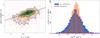 |
Fig. B.1
left panel: distribution of the [N ii]/Hα line ratio along the B − V colour for all the detected H ii regions. The image and contours show the density distribution in this space of parameters. The first contour is at the mean density, with a regular spacing of four times this value for each consecutive contour. The solid line shows the actual regression found between the two represented parameters. Right panel: histograms of the relative difference between the Hα intensity derived from the narrow band images described in Sect. 3, and the ones derived from the fitting technique over the extracted spectra, described in Sect. 6.1, before (blue-solid histogram) and after (red-shaded histogram) applying the correction from the [N ii] contamination based on the correlation shown in the left-panel. |
| Open with DEXTER | |
The Hα luminosity observed in spiral and irregular galaxies is believed to be a direct tracer of the ionization of the inter-stellar medium (ISM) by the ultraviolet (UV) radiation which is produced by young high-mass OB stars. Since only high-mass, short-lived, stars contribute significantly to the integrated ionizing flux, this luminosity is a direct tracer of the star formation rate (SFR), independent of the previous star formation history. This is why dust-corrected Hα luminosity is one of the most widely used observables to derive SFR in galaxies.
Among the several methods used to derive the Hα luminosity and its distribution across the optical extension of the galaxies, narrow-band image is by far the cheapest one in terms of telescope time and complexity. Thus, it is the most frequently used too (e.g., James et al. 2004; Pérez-González et al. 2003). The technique is rather simple: (i) the galaxy is observed using both a narrow-band filter centered at the wavelength of Hα and a broader filter covering a wider range around the same wavelength range; (ii) The broad-band image is used to correct for the underlying continuum and provide a relative flux calibration of the continuum subtracted narrow-band image; (iii) by performing a flux calibration of the broad-band image it is possible to have an accurate calibration of the decontaminated Hα emission map.
One of the major limitations of narrow-band Hα imaging is contamination by the [N ii] line doublet, which can hardly be derived from a single narrow-band imaging (e.g. James et al. 2005). Most frequently used narrow-band filters have a width of ~50−80 Å, and in most of the cases the emission from the [N ii] λλ6548, 6583 contaminate the derived Hα emission map, and therefore, the derived Hα luminosity and SFR. Despite of the fact that the [N ii]/Hα line ratio present a strong variation across the field for star-forming galaxies (e.g. Sánchez et al. 2011, and Fig. 7), it is generally assumed an average correction.
The most commonly used corrections for entire galaxies are those derived by Kennicutt (1983) and Kennicutt & Kent (1983). Spectrophotometric [N ii]/Hα ratios of individual extragalactic H ii regions from the literature (see Kennicutt & Kent 1983, and references therein) were compiled from 14 spiral galaxies (mostly of type Sc) and 7 irregular galaxies. The average Hα/(Hα + [N ii]) ratio was found to be fairly constant, spanning the ranges 0.75 ± 0.12 for the spirals, and 0.93 ± 0.05 for the irregulars (Kennicutt 1983). In terms of the ratio [N ii]-total/Hα this corresponds to a median value of 0.33 for spirals and 0.08 for irregulars. These values were calculated by finding the [N ii]-total/Hα ratio of the brightest H ii regions, averaging for each galaxy and then determining the mean value for spiral and irregular types. This implicitly assumes that all H ii regions have the same proportion of [N ii]-total to Hα emission as those regions measured. We have already illustrated that this may not be the case in general, e.g., Fig. 7. However, recent results show that the total integrated spectra of galaxies may have a stronger [N ii] emission than the one reported before, with a large variation line ratios for different galaxy types Kennicutt (1992).
Jansen (2000) already showed that there is a trend of the average [N ii]/Hα ratio with galaxy luminosity. In their study, the lines ratios for galaxies brighter than MB = −19.5 are in agreement with the values found by Kennicutt (1992), but fainter than this a striking trend is seen towards much lower values of this ratio. A similar trend is found by Gavazzi et al. (2004).
To our knowledge the only attempt to make a correction across the optical extension of each galaxy is the one introduced by James et al. (2004). In this study they used the spatial distribution of the [N ii]/Hα line ratio, instead of an average correction for all the entire galaxy. However, their estimations of the distribution of the line ratio are based on physical principles rather than in direct measurements.
Making use of our extensive catalogue of individual emission line regions, we have explored possible empirical corrections that allow us to perform spatially resolved corrections across the optical extension of each individual galaxy. For doing so we correlated the measured [N ii]/Hα line ratios for each individual region with different parameters easy to address using broad-band photometry, like the Hα intensity, B and V-band magnitudes, B − V colours and radial distance relative to the effective radius.
Among the different explored linear relations, the one with stronger correlation coefficient (r ~ 0.5), and better defined zero-point and slope, was the one with the B − V colour:  (B.1)Figure B.1, left panel, shows the distribution of [N ii]/Hα line ratios along the B − V colour for all the detected H ii regions. The image and contours show the density distribution in this space of parameters, together with a solid line showing the best fitted linear regression described before. This relation can be used as a simple proxy of the [N ii]/Hα line ratio, and used to decontaminate the described Hα narrow-band images.
We applied the proposed correction to the Hα narrow-band images described in Sect. 3, to demonstrate its improvement over a classical single correction over the entire galaxy. We derive for each detected H ii region the corresponding flux in the Hα narrow-band images, using the segmentation maps provided by HIIexplorer (Hαimg). Then, we obtain the relative difference between this contaminated flux and the real Hα flux measured using the fitting procedure describe in Sect. 6.1. The mean value of this difference is ~0.28 ± 0.19, which is consistent with the typical average correction found in the literature (e.g., Kennicutt 1983). Figure B.1, right panel, shows a solid-blue histogram of the relative difference between the Hα flux derived from the narrow-band images, and the ones derived using the emission line fitting procedure after applying this average correction.
The derived correction is then applied on the same data using a iterative processes. In each iteration the B − V colour is used to guess the [N ii]/Hα line ratio. This ratio, together with the decontaminated Hα flux derived from in the previous iteration, is used to derive the [N ii] intensity. Finally, this intensity is subtracted to the original contaminated Hαimg intensity to derive a new decontaminated flux. For the first iteration it is assumed that the intensity decontaminated by the average correction is a good starting estimation of the Hα flux. After three iterations the decontaminated Hα flux converge with a few percent. Figure B.1, right panel, shows a hashed-red histogram of the relative difference between the the Hα flux derived from the narrow-band images, and the ones derived using the emission line fitting procedure after applying the proposed correction. It is clear that the new histogram has a lower dispersion that the previous one, with a standard deviation of ~0.15. The proposed correction improves the accuracy of the derived Hα intensity by a a ~60%, in average.
The effect of this correction is stronger when analysing the spatial distribution of the Hα emission and/or the relative strength of the SFR. As we already indicated the [N ii]/Hα ratio tends to decrease with the radius. Therefore, an average correction would overestimate the Hα emission and the SFR in the inner regions, and underestimate it in the outer ones. Indeed, some authors have corrected the image-based Hα fluxes for [N ii] contamination using available spectroscopical data of selected H ii regions within the galaxy (e.g. López-Sánchez & Esteban 2008).
So far, we did pay no attention to the possible physical connections between the explored parameters. The described relation may indicate a physical connection between the conditions of the ionized gas and the ionizing stellar population, or between both of them and a third parameter not considered here. A possible origin of this connection could be a co-evolution of both components of the H ii regions. The study of this connection, that we will address in future works, is beyond the scope of the current analysis.
© ESO, 2012
Current usage metrics show cumulative count of Article Views (full-text article views including HTML views, PDF and ePub downloads, according to the available data) and Abstracts Views on Vision4Press platform.
Data correspond to usage on the plateform after 2015. The current usage metrics is available 48-96 hours after online publication and is updated daily on week days.
Initial download of the metrics may take a while.