| Issue |
A&A
Volume 564, April 2014
|
|
|---|---|---|
| Article Number | A57 | |
| Number of page(s) | 20 | |
| Section | Stellar structure and evolution | |
| DOI | https://doi.org/10.1051/0004-6361/201323031 | |
| Published online | 04 April 2014 | |
Rotating massive O stars with non-spherical 2D winds⋆
1 Armagh Observatory, College Hill, Armagh BT61 9DG, UK
e-mail: This email address is being protected from spambots. You need JavaScript enabled to view it.
2 School of Physical and Geographical Sciences, Lennard-Jones Laboratories, Keele University, Staffordshire, ST5 5BG, UK
Received: 11 November 2013
Accepted: 19 February 2014
Abstract
We present solutions for the velocity field and mass-loss rates for 2D axisymmetric outflows, as well as for the case of mass accretion through the use of the Lambert W-function. For the case of a rotating radiation-driven wind the velocity field is obtained analytically using a parameterised description of the line acceleration that only depends on radius r at any given latitude θ. The line acceleration g(r) is obtained from Monte-Carlo multi-line radiative transfer calculations. The critical/sonic point of our equation of motion varies with latitude θ. Furthermore, an approximate analytical solution for the supersonic flow of a rotating wind is derived, which is found to closely resemble the exact solution. For the simultaneous solution of the mass-loss rate and velocity field, we use the iterative method of our 1D method extended to the non-spherical 2D case. We apply the new theoretical expressions with our iterative method to the stellar wind from a differentially rotating 40 M⊙ O5–V main sequence star as well as to a 60 M⊙ O-giant star, and we compare our results to previous studies that are extensions of the Castor et al. (1975, ApJ, 195, 157) CAK formalism. Next, we account for the effects of oblateness and gravity darkening. Our numerical results predict an equatorial decrease of the mass-loss rate, which would imply that (surface-averaged) total mass-loss rates are lower than for the spherical 1D case, in contradiction to the Maeder & Meynet (2000, A&A, 361, 159) formalism that is oftentimes employed in stellar evolution calculations for rotating massive stars. To clarify the situation in nature we discuss observational tests to constrain the shapes of large-scale 2D stellar winds.
Key words: hydrodynamics / methods: analytical / stars: early-type / stars: mass-loss / stars: rotation / methods: numerical
Appendix A is available in electronic form at http://www.aanda.org
© ESO, 2014
1. Introduction
In recent years considerable progress has been made in our theoretical modelling of rotating massive stars (Maeder & Meynet 2012; Langer 2012) and our basic understanding of spherical radiation-driven winds (Puls et al. 2008). However, in order to get a grasp on the non-spherical 2D outflows of rotating massive stars, involving B[e] supergiants (Zickgraf et al. 1985), classical Be stars (Porter & Rivinius 2003) as well as luminous blue variable (LBV) outflows (Groh et al. 2006), it is paramount to combine the intrinsically 2D nature of rotation and mass loss (e.g. Lovekin 2011; Espinosa & Rieutord 2013). This is not only required for a basic understanding of massive star evolution, but also for linking the oftentimes non-spherical supernova (SN) data with their progenitors (e.g. Maund et al. 2007; Hoffman et al. 2008).
We need to develop 2D wind models in order to obtain a physical understanding of how rotation might affect both the strength and latitudinal dependence of their outflows. In turn winds may be able to remove significant quantities of angular momentum, potentially down to masses as low as 10–15 M⊙ (Vink et al. 2010). Whether the mass loss originates from the pole or the equator remains currently unknown. Yet, is of paramount importance for understanding whether rapid rotation is maintained or leads to stellar spin loss (Meynet & Maeder 2007), highly relevant for our understanding of the progenitor evolution of long-duration gamma ray bursts (GRBs).
Previous models of the winds from rotating stars have mostly been 1D models of the equatorial flow versus the polar flow, although one 2D numerical calculation has been performed by Poe (1987). The 1D model of Friend & Abbott (1986, hereafter FA) concerned the influence of stellar rotation on the hydrodynamics of a stellar wind, involving a solution of the fluid equations in the equatorial plane, which included centrifugal forces. They used a form of the radiation force after Castor et al. (1975, hereafter CAK), but corrected for the finite angular size of the stellar “disk” (see also Pauldrach et al. 1986).
Bjorkman & Cassinelli (1993, hereafter BC) provided an analytical approximation for the axisymmetric 2D supersonic solution (i.e. for the velocity field and density distribution) of a rotating radiation-driven wind, obtained from the FA 1D model of the equatorial flow. In order to find the streamline trajectories, they rotated the FA 1D solution (in the equatorial plane) up to the initial co-latitude θ0 of the streamline at the stellar surface, adjusting the equatorial rotation velocity of the central star vrot by vrotsinθ0. The supersonic solutions obtained this way provided the velocity and density as a function of θ0 and radius r, i.e. in a non-explicit form: given a location (r,θ), one needs to find θ0 of the streamline that passes through that location, by iteratively solving additional equations. As a result, they explained how rotation can lead to the production of a dense equatorial disk around, e.g. Be stars, by means of their wind-compressed disk (WCD) model.
Refinements of the BC model have been also made for simulating the density structure of rotating O-star winds (e.g. Petrenz & Puls 1996). Owocki et al. (1996) showed that the inclusion of non-radial line forces leads to a small polarwards vθ component, which may inhibit disk formation in Be stars. Moreover, Maeder (1999) showed that gravity darkening as a result of the Von Zeipel (1924) effect will generally lead to a polar wind. It should be noted that the hydrodynamical wind models of Owocki and colleagues that lead to polar winds employ an approximated line driving formula from CAK for 1D.
A generally prolate wind structure was however confirmed by the sectorial 1.5D wind models of Pelupessy et al. (2000) that employed 1D detailed Monte Carlo line acceleration computations of Vink et al. (1999). In their models for B[e] supergiants, Pelupessy et al. also showed that when models are in close proximity to the bi-stability jump it is possible to overcome the polar enhancement due to the Von Zeipel effect, and drive equatorial enhancements, as originally suggested by Lamers & Pauldrach (1991) for Be and B[e] supergiant disk formation. Cure et al. (2005) and Madura et al. (2007) derived 1D hydrodynamical models for very rapid rotators (above 75% of the critical rate) finding a slow solution to the classical CAK theory, which may enable disk formation in Be stars and B[e] supergiants, when accounting for the wind bi-stability effects of Vink et al. (1999). However, again, these models employ a simplified treatment of the line acceleration due to the 2 (or 3) parameter power-law approximation due to CAK. What is eventually required in order to resolve the intricate problem of stellar rotation with mass loss are 3D Monte Carlo radiative transfer calculations in combination with a full hydrodynamic solution. Most published models have necessarily made significant assumptions with respect to either the line-force calculations or the wind hydrodynamics.
We suggested a new parametrisation of the line acceleration (Müller & Vink 2008, hereafter Paper I), expressing it as a function of radius rather than of the velocity gradient as in CAK theory. The implementation of this formalism allowed for local dynamical consistency as we were able to determine the momentum transfer at each location in the wind through the use of Monte Carlo simulations. In Muijres et al. (2012), we tested our hydrodynamic wind solutions and velocity laws by additional explicit numerical integrations of our fluid equation, also accounting for a temperature stratification. These results were in excellent agreement with both our full and our approximated solutions from Paper I. We here build on those results, now deriving analytical solutions for the 2D case concerning both the velocity and density structure in an axisymmetric mass outflow (or inflow) scenario. Furthermore, we extend our iterative method from Paper I for the simultaneous solution of the mass-loss rate and velocity field to the 2D case of a rotating non-spherical stellar wind.
We obtain the velocity field fully analytically without any previous fits to numerical solutions of the fluid equation of FA, if we neglect the polar velocity vθ in our model. We are justified in doing so as long as the stellar rotation speeds are well below the critical value where disks are formed, that is, for example for O-star winds, where non-spherical outflows have only been detected in a small (~20%) minority only involving “special” O-type sub-groups (Oe, Onfp) from linear spectropolarimetry observations (Harries et al. 2002; Vink et al. 2009).
However, the non-spherical problem for the flow in the equatorial plane including the case of the outflow at the pole (where vθ ≡ 0 for symmetrical reasons) are as well fully analytically solved by our improved 2D wind model without any restrictions to the velocity components and the rotational speed of the central star. For the specific case of a non-spherical radiation-driven wind, we do not rely on the CAK expression for the radiation force, rather we describe the line acceleration as a function of stellar radius g(r,θ) at a given constant co-latitude θ. In addition, the critical point of our stellar wind is the sonic point (depending on latitude) and not the CAK critical point. The calculation of g(r,θ) is performed through Monte Carlo simulations accounting for multi-line transfer, and the wind parameters are solved simultaneously – in an iterative way – for each latitude of interest.
The set-up of the paper is as follows. In Sects. 2.2–2.5, the hydrodynamic equations for a non-spherical axisymmetric steady flow are introduced including a derivation of the mathematical description of the radiative line acceleration as a function of radius for the case of a rotating radiation-driven wind. The process for obtaining the fully analytical 2D solutions is described and discussed in Sect. 2.6. Here, the velocity field for the entire family of solutions is provided in an explicit general expression from which the solutions for a rotating radiation-driven wind or mass accretion flux (e.g. collapsing protostellar cloud) follow as unique trans-sonic solutions through the critical point. Moreover, an approximate analytical solution for the supersonic flow is presented. In Sect. 3, we describe our numerical computation obtaining the radiative acceleration in our stellar wind models. Furthermore, our iterative method for the determination of the consistent solution for the mass-loss rate in case of a spherical wind is being extended and applied to the wind from a rotating star. In Sect. 4, we present the application of our models to a differentially rotating stellar wind from a typical 40 M⊙ O5–V-star, including the effects of oblateness and gravity darkening, and from a rotating 60 M⊙ O-giant star. We discuss the results, before we summarise and discuss our findings in Sect. 5.
2. Radiation hydrodynamics of rotating and expanding or collapsing systems
2.1. The velocity field
The velocity field of the differentially rotating system at location r = (r, θ, φ) can generally be described by its spherical components  (1)with the unit vectors er, eθ, eφ, in radial, polar and azimuthal direction, respectively, where the following two presentations of the unit vectors
 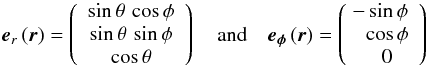 (2)will be useful1.
2.2. Basic equations of hydrodynamics
Considering the particular chosen system as a non-viscous2, i.e., ideal fluid, the momentum equation 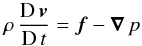 (3)is valid (see, e.g., Mihalas & Weibel Mihalas 1984), where D/D t is the covariant Lagrangean or co-moving time derivative in the fluid-frame of a material element and v is its velocity, f is the total external body force per volume acting on a mass element of fluid, and ∇ p is the divergence term of a diagonal isotropic stress tensor ∇·T, in which T = −p I and p is the hydrostatic pressure.
One also needs to consider the equation of continuity 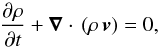 (4)with the covariant divergence ∇·v of the velocity vector.
2.3. Simplifying assumptions
Besides the assumption of an inviscid flow and to account for the axisymmetric and stationary problem, we make the further following simplifying assumptions to solve the hydrodynamic equations analytically:
-
1.
The stellar wind (flow) is first assumed to be isothermal to derivethe analytical expressions for the hydrodynamic solutions. In thiscase, the equation of state
 (5)is valid, where a is the isothermal speed of sound and ρ is the density of the wind (system). This assumption, however, will be relaxed later by applying our iterative method (described in Sect. 3), to compute the mass-loss rates and the parameters in our analytical wind solutions consistently with the radiation field and ionisation/excitation state of the gas of an outflowing stellar model atmosphere in non local thermodynamic equilibrium, assuming radiative equilibrium, by the use of the ISA-Wind code allowing a temperature stratification3. Additionally, in Muijres et al. (2012), we verified our hydrodynamic solutions, especially for the case of a spherical wind without rotation, by explicit numerical integrations of our fluid equation also accounting for a temperature distribution.
 -
2.
We assume a stationary axisymmetric flow, since we are interested in a rotating star (system) where rotational effects dominate the flow, i.e. we set
 (6)and therefore disregard shocks as well. Furthermore, we exclude the presence of clumps.
 -
3.
For symmetrical reasons, the polar component of the flow velocity should be
 (7)as well as the polar and azimuthal force components,
  (8)and
  (9)respectively, in the equatorial plane and at the pole for an axisymmetric flow. At the pole, the hydrodynamic solutions must pass over into those for the spherical case without rotation. Eqs. (7) to (9) allow us then the seperation of the radial motion for any individual latitude. However, for intermediate latitudes, these approximations do generally not hold: for instance, neglecting the meridional velocity there, restricts the application of our model only to those cases where matter exchange between layers of different latitude (and therefore also the occurrance of a friction between) can be neglected. We therefore apply our model, in the case of stellar winds, only to rotating O-stars with rotational speeds below the critical value where disks are formed. Moreover, the additional involvement of the distortion of a central star due to its rotation (and consequently the effect of gravity darkening as well) in the course of our investigations, may result in a non-vanishing radiative force fθ in θ-direction at all mid-latitudes. Therefore, for winds from those rotating O-stars, we employ our formalism and method (in Sect. 4) exlusively only on the equatorial plane and the pole, to compute the more accurate wind parameters and mass-loss rates there, where the above assumptions (Eqs. (7)–(9)) are satisfied best4. Then, at latitudes between the pole and equator, all corresponding hydrodynamic quantities adopt values which lie in-between these two extreme values (constraints).
 -
4.
In the case of a wind from a luminous early-type star, the wind is primarily driven by continuum plus line radiation forces, where the radial acceleration on a mass element is
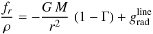 (10)with
  (11)the force ratio between the radiative acceleration
  due to the continuum opacity (dominated by electron scattering) and the inward acceleration of gravity g. Γ is supposed to be independent of radius r, may however vary with polar angle θ, and
  is the outward radiative acceleration due to spectral lines. M is the mass of the central star.
2.4. Simplified hydrodynamic equations
2.4.1. Wind density and mass-loss rate
If we use the covariant derivative (see Mihalas & Weibel Mihalas 1984), for spherical coordinates and apply assumptions 2 and 3 to the equation of continuity (4), we find 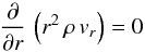 (12)for a two-dimensional axisymmetric and steady flow.
This equation looks the same as that one, we would get for a one-dimensional, spherically symmetric and steady flow, however, this expression is quite more general and only fulfilled for a given constant polar angle θ. But similar to a spherically symmetric flow, the integration of Eq. (12) yields  (13)in which here Ṁ(θ) is not the total mass flux through a spherical shell surrounding the star, but its mass flux (or mass-loss rate) at co-latitude θ through the star surface multiplied by 4 π R2 (cf. definition in BC) that is conserved for each angle θ. The value of Ṁ (θ) can later be determined by the given values of velocity vr (R,θ) and density ρ (R) at the stellar radius R (or at the surface of an inner core).
The total mass-loss rate must then be 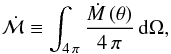 (14)integrated over the solid angle Ω. Note that in case of a collapsing system (e.g. protostellar cloud) this mass-loss rate is negative, because the inner core gains mass.
Finally, by Eq. (13), we obtain the 2D density distribution 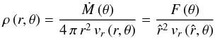 (15)at location (r,θ), with the defined flux F = Ṁ (θ)/4 π R2 through the star’s surface at radius R and the dimensionless radius
  .
.
Please note that all formulae derived in this Sect. 2 are expressed in terms of  referring to the radius R, which is (throughout this section) the stellar (i.e. photospheric) radius of the central star (or the inner core radius of any central object, respectively). However, all formulae can generally also be applied with respect to the reference radius R to be the inner boundary radius Rin, from where the numerical computations of the (stellar wind) model start.
2.4.2. The azimuthal velocity component and the correction for oblateness
By using the correct contravariant components of acceleration (D vi/D t) in Eq. (3), for spherical coordinates, and replacing them by their equivalent physical components (see again, e.g., Mihalas & Weibel Mihalas 1984), and applying assumptions 1–4, we obtain the simplified r- and φ-component of the momentum equation
 with the external radial force per unit mass fr, i.e. the radial acceleration on the mass element in Eq. (10), in case of a stellar wind.
The φ-component of the momentum Eq. (17) is nothing more than the conservation of angular momentum per unit mass 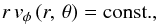 as one would expect for external central forces and axisymmetry, what we have, of course, supposed before. Then, the last differential Eq. (17) can be solved (i.e. integrated) immediately and separately from Eq. (16), to obtain the unknown velocity component vφ
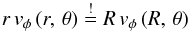 by choosing an adequate boundary (initial) condition
 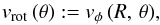 (18)i.e. rotational speed of the star (inner core) surface at co-latitude θ.
Hence, the φ-component of the velocity of a particle at distance in its orbit, originating from the stellar surface at co-latitude θ and ejected with vrot (θ), remaining on the cone surface of constant angle θ, becomes 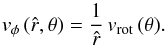 (19)Assuming that the central star surface (or inner core surface) behaves like a rotating rigid sphere (R = const.), the rotational velocity at co-latitude θ would then be described by
  (20)with the equatorial rotation speed Vrot.
However, due to rapid rotation, the central star (core) can become oblate from the centrifugal forces and can then be described as a rotating rigid ellipsoid (R = R(θ)) with rotational velocity  (21)at co-latitude θ, where Req is the radius R(θ = π/2) at the equator.
Here, the stellar (core) radius R(θ), depending on latitude and rotation speed is given by (Cranmer & Owocki 1995, hereafter CO; Petrenz & Puls 1996, hereafter PP)  (22)where Rp is the polar radius and assumed to be independent of the rotational velocity, i.e. used as stellar input parameter, and Ω is the normalised stellar angular velocity and defined by
  (23)with the critical angular velocity
  (24)and equatorial radius
  (25)Note that the above definition of ωcrit differs from the break-up velocity ωcrit,spherical = vcrit/Rp introduced in the following Sect. 2.4.4, where the rotational distortion of the stellar surface is neglected.
2.4.3. The effect of gravity darkening
If one considers the distortion of the central star due to its rotation, one also has to account for the effect of gravity darkening caused by its oblateness. The early work of von Zeipel (1924) for distorted stars states that the radiative flux F (θ) emerging from the surface at co-latitude θ is proportional to the local effective gravity  (26)Therein the normal component of gravity is (see Collins 1965; or PP)
 ![Mathematical equation: \begin{eqnarray} \label{g-perp-eq} g_{\perp}\,(\Omega(V_{\rm rot}),\theta) & = & \frac{G M}{R_{\rm p}^{2}}\, \frac{8}{27} \left[ \left( \frac{27}{8}\, \left(\frac{R_{\rm p}}{R(\theta)}\right)^{2} - \frac{R(\theta)}{R_{\rm p}}\, \Omega^2\, \sin^{2}\theta \right)^2 \right. \nonumber \\ & & + \left. \Omega^4\, \left( \frac{R(\theta)}{R_{\rm p}}\right)^{2}\, \sin^{2}\theta \, \cos^{2}\theta \right]^{1/2} , \end{eqnarray}](/articles/aa/full_html/2014/04/aa23031-13/aa23031-13-eq85.png) (27)with the stellar radius R(θ) in Eq. (22), and the proportional constant
(27)with the stellar radius R(θ) in Eq. (22), and the proportional constant  (28)is given by the constraint that the surface-integrated flux is equal to the total luminosity L of the (oblate) star, where
 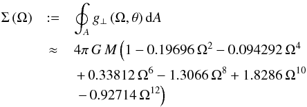 (29)is the surface-integrated gravity (see the power series in CO).
Together with the use of the Stefan-Boltzmann law for the flux emitted at co-latitude θ (30)where σB is the Boltzmann constant, we obtain finally the following equation for the local effective temperature
 ![Mathematical equation: \begin{equation} \label{local-eff-T-eq} T_{\rm eff}\,(V_{\rm rot},\theta{}) = \left[ \frac{L}{\sigma_{B}\,\Sigma\,(V_{\rm rot})}\, g_{\perp}\,(V_{\rm rot},\theta) \right]^{1/4} . \end{equation}](/articles/aa/full_html/2014/04/aa23031-13/aa23031-13-eq92.png) (31)Through the angular velocity Ω (cf. Eq. (23)), the local effective temperature in Eq. (31) and the stellar radius R(θ) in Eq. (22) depends also on the continuum Eddington factor Γ (cf. Eq. (11)) which is, in case of an homogeneous spherical star,
(31)Through the angular velocity Ω (cf. Eq. (23)), the local effective temperature in Eq. (31) and the stellar radius R(θ) in Eq. (22) depends also on the continuum Eddington factor Γ (cf. Eq. (11)) which is, in case of an homogeneous spherical star,  (32)where σe is the electron scattering cross-section.
Then, this Eq. (32) is also used in our case to calculate a mean value of  from the prescribed value of L of the non-spherical star, to be able to evaluate Eq. (22) and Eq. (31) for the stellar parameters R(θ) and Teff (θ) at a given co-latitude θ of interest.
However, since the effective gravity and therefore the flux vary over the surface of the rotating star, we still need to determine the local value of Γ (θ) of the non-spherical star that can be defined as  (33)by means of the definition of the latitude-dependent luminosity
 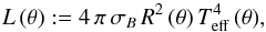 (34)which is the luminosity of a corresponding spherical star with radius R(θ) and effective temperature Teff (θ) of the considered non-spherical star at co-latitude θ.
2.4.4. The equation of motion
Next, we wish to solve the r-component of the momentum Eq. (16), i.e. find an expression for the radial velocity component vr of the non-spherical axisymmetric steady flow. Equation (16) can then be rewritten 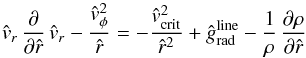 (35)in non-dimensional form. In which the following dimensionless velocities (in units of the isothermal sound speed a)
 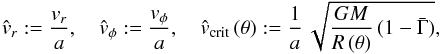 (36)and dimensionless line acceleration
 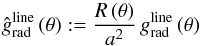 (37)are used, where vcrit (θ = 0) equals the break-up velocity of the rotating central object (usually without consideration of radiative line acceleration terms and rotational distortion). By means of Eq. (15) and applying the chain rule to the function
  , we obtain
 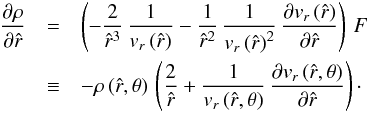 Using this expression for
  in Eq. (35) together with our relation for the azimuthal velocity, Eq. (19), we finally find the dimensionless differential equation of motion (EOM) for the radial velocity at constant co-latitude θ
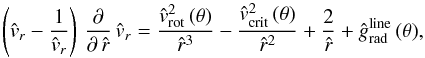 (38)that is now independent of ρ.
2.5. The line acceleration term and the final equation of motion
 |
Fig. 1 Dimensionless radiative line acceleration |

To derive a sophisticated mathematical expression for the radiative line acceleration  at a constant co-latitude θ of interest as a function of radius r only, we demand the same physically motivated mathematical properties as described in Paper I (as for the case of a radiation-driven spherical wind):
  (39)This function is independent of
  and (
and ( ) and dependent on only, at constant co-latitude θ. Note that, herein, the set of four parameters all depend on latitude: ĝ0 = ĝ0(θ),
  , γ = γ(θ), δ = δ(θ), due to the rotation of the central star.
The line force is zero at radius  near the stellar photosphere (
 ) and everywhere else positive for
  . To guarantee the decrease of
  as
as  with increasing radial distance from the central star at intermediate radii (at the right side of the
  peak) in particular, we had to introduce the parameter δ in addition to γ (where 0 < γ ≲ 1 and 0 < δ ≲ 1).
Hence, the equation of motion (38) for each latitude becomes  (40)vrot is the azimuthal velocity of the surface of the inner rotating star (object) at co-latitude θ of interest. This equation is fully solvable analytically as in the spherical case without rotation (cf. Paper I).
2.6. Analytical solutions of the equation of motion
2.6.1. The critical point and critical solutions
 |
Fig. 2 Topology of solutions |


The EOM (Eqs. (38) and (40)) yields several families of solutions that have quite different mathematical behaviour and physical significance (cf. Fig. 2).
The left hand side of Eq. (40) vanishes for  at the critical radius
  , where
  . That is, the critical point velocity here is equal to the isothermal sound speed
  , and the critical radius is just the sonic radius
  (41)as is also the case for thermal winds or mass accretion events (where
  ).
).
We are now interested in under which conditions one can obtain a continuous and smooth trans-sonic flow through the critical point  of Eq. (40). For the case of a stellar wind, this means how to obtain a smooth transition from subsonic and subcritical flow (
 ) at small
  to supercritical and supersonic flow (
 ) at large
  , when this critical solution has a finite positive slope (
 at
at  (cf. solid curve 1 in Fig. 2)? 5 Then, it is evident from the left hand side of Eq. (40) that one can obtain such a trans-sonic wind, if the right hand side (1) vanishes at the critical radius , (2) is negative for , and (3) is positive for .
The opposite situation occurs for the case of mass accretion in e.g. a collapsing cloud. If ( , we obtain the second unique trans-sonic and critical solution in which
  is monotonically decreasing from supersonic speeds for
  , e.g. near the protostar, to subsonic speeds for
  at the outer edge of the cloud (see also the second solid line 2, in Fig. 2, for the case of a corresponding accretion flow with a star as the central object).
Here we are mainly interested in the critical wind solution of Eq. (40). The right hand side of Eq. (40) vanishes at the critical radius  that solves the equation
  (42)Therefore, the critical radius (for each latitude) has to be determined numerically by means of the above equation and the line term parameters
  , γ, δ and
  , depending on the rotational speed Vrot of the central object. However, if one assumes values of γ and δ close to 1, one can provide a good analytical approximation (for the solution of Eq. (42)) for the critical radius
  (43)if the rotation speed at co-latitude θ fulfills the condition
  For the simpler case of a thermal wind (or any other non line-driven mass flow), where can be set to zero (in Eq. (42)), we obtain the analytical solution
  (44)Equation (44), and Eq. (43) under the assumption of a constant remaining line force (i.e. value), imply that the critical radius moves closer to the inner core radius (at any latitude besides of that of the pole) with increasing rotational speed Vrot for these particular cases of a trans-sonic flow.
2.6.2. Solving the equation of motion
The equation of motion (40) can be solved by first integrating the left hand side over , and then integrating the right hand side over , separately, which yields  (45)with the right hand side of Eq. (45) denoted as the function
  (46)with the constant of integration C, that is determined by the boundary condition of the radial velocity
  at a given location
  .
.
From Eq. (45), we can determine  for the solution that passes through the particular point
  ,
,  (47)Therefore the function f in Eq. (46) becomes
 ![Mathematical equation: \begin{eqnarray} \label{func-f} f\,({\hat r},\theta; {\hat r}',{\hat v_{r}}') & = & {\hat v_{r}}'^{2} - \ln{\hat v_{r}}'^{2} + 2\,{\hat v}_{\rm crit}^{2} \left( \frac{1}{\hat r} - \frac{1}{\hat r'}\right) + 4\,\ln\left(\frac{\hat r}{\hat r'}\right) \nonumber\\ & & +\, \frac{2}{\hat r_{0}}\,\frac{\hat g_{0}}{\delta\left(1+\gamma\right)} \left[ \left( 1 - \frac{\hat r_{0}}{{\hat r}^{\delta}}\right)^{1 + \gamma} - \left( 1 - \frac{\hat r_{0}}{{\hat r}'^{\delta}}\right)^{1 + \gamma} \right] \nonumber\\ & & +\, {\hat v}_{\rm rot}^{2} \, \left( \frac{1}{{\hat r}'^2} - \frac{1}{{\hat r}^2}\right) \cdot \end{eqnarray}](/articles/aa/full_html/2014/04/aa23031-13/aa23031-13-eq178.png) (48)And from this, Eq. (45) now reads
(48)And from this, Eq. (45) now reads  or, equivalently,
  (49)which is solved explicitly and fully analytically in terms of the Lambert W function (cf. Corless et al. 1993, 1996).
2.6.3. The solution(s) of the equation of motion
It is now possible to provide an explicit analytical expression for the solution of the equation of motion (40), or Eq. (49), by means of the W function (cf. Paper I). If we compare Eq. (49) with the defining equation of the Lambert W function  (50)we find that
  or
or  (51)is the general solution of the equation of motion that passes through the point , with the argument function of the W function
  (52)Since the argument of the W function in Eq. (51) is always real and negative, it is guaranteed that the argument of the square root never becomes negative, and hence the solution is always real.
Inserting  from Eq. (48) into Eq. (52) yields
 ![Mathematical equation: \begin{eqnarray} \label{x-gensol} x\,({\hat r},\theta; {\hat r}',{\hat v_{r}}') & = & - \left( \frac{\hat r'}{\hat r} \right)^4 {\hat v_{r}}'^{2} \exp \left[ - {\hat v}_{\rm rot}^{2} \, \left( \frac{1}{{\hat r}'^2} \!-\! \frac{1}{{\hat r}^2}\right) -2\, {\hat v}_{\rm crit}^{2}\, \left( \frac{1}{\hat r} \!-\! \frac{1}{\hat r'} \right) \right. \nonumber\\[2mm] & & \hspace{-4ex} \left. -\frac{2}{\hat r_{0}} \frac{\hat g_{0}}{\delta\left(1+\gamma\right)} \left( \left( 1 - \frac{\hat r_{0}}{{\hat r}^{\delta}}\right)^{1+\gamma} - \left( 1 - \frac{\hat r_{0}}{{\hat r}'^{\delta}}\right)^{1+\gamma}\right) - {\hat v_{r}}'^{2} \right] \end{eqnarray}](/articles/aa/full_html/2014/04/aa23031-13/aa23031-13-eq187.png) (53)the general expression for the argument function x depending on the parameters .
(53)the general expression for the argument function x depending on the parameters .
Thus, for the trans-sonic case of a stellar wind or general accretion flow, where  and
and  , the analytical solution is
  (54)with
 ![Mathematical equation: \begin{eqnarray} \label{x-windsol} x\,({\hat r},\theta) & = & - \left( \frac{\hat r_{\rm c}}{\hat r} \right)^4 \, \exp \left[ - {\hat v}_{\rm rot}^{2} \, \left( \frac{1}{{\hat r_{\rm c}}^2} - \frac{1}{{\hat r}^2}\right) -2\, {\hat v}_{\rm crit}^{2}\, \left( \frac{1}{\hat r} - \frac{1}{\hat r_{\rm c}} \right) \right. \nonumber\\[2mm] & & \left. -\frac{2}{\hat r_{0}} \frac{\hat g_{0}}{\delta\left(1+\gamma\right)} \, \left( \left( 1 - \frac{\hat r_{0}}{{\hat r}^{\delta}}\right)^{1\,+\,\gamma} - \left( 1 - \frac{\hat r_{0}}{{\hat r_{\rm c}}^{\delta}}\right)^{1\,+\,\gamma} \right) - 1 \right] . \end{eqnarray}](/articles/aa/full_html/2014/04/aa23031-13/aa23031-13-eq192.png) (55)We are only interested in the possible two real values of W(x), the k = 0, − 1–branches in Eq. (51) or Eq. (54), where x is real and −1/e ≤ x < 0. The branch point at x = −1/e, where these two branches meet, corresponds to the critical point , where the velocity in Eq. (54) becomes
(55)We are only interested in the possible two real values of W(x), the k = 0, − 1–branches in Eq. (51) or Eq. (54), where x is real and −1/e ≤ x < 0. The branch point at x = −1/e, where these two branches meet, corresponds to the critical point , where the velocity in Eq. (54) becomes  ≡ 1. Depending on which branch of W one is approaching this point x = −1/e, one obtains a different shape of the
  –curve, i.e. a stellar wind or a collapsing system.
However, to determine which of the two branches to choose at a certain range of radius between ![Mathematical equation: \hbox{$[1, {\hat r}_{\rm c}]$}](/articles/aa/full_html/2014/04/aa23031-13/aa23031-13-eq199.png) and
and  as to guarantee a continuous, monotonically increasing, and smooth trans-sonic flow (as, e.g., in the case of a stellar wind), one needs to examine the behaviour of the argument function
  of W, in Eq. (55), with radius at a given co-latitude θ. Then, the argument function decreases monotonically from the stellar radius
  (with value of nearly zero) to its minimum at with x = −1/e to afterwards increase monotonically again.
Finally, a detailed investigation (cf. Paper I) yields the following amount of the radial velocity component (i.e. the axisymmetric two-dimensional trans-sonic analytical solution of our equation of motion for a rotating and expanding or collapsing system) for a given latitude, i.e. polar angle θ
-
(a)
for the case of a stellar wind, and Eq. (54) (and thepositive sign in front of the root) with the argument function inEq. (55), choosing the branch
![Mathematical equation: \begin{equation} \label{k-branch-wind} k = \left\{ \begin{array}{ccc} \,\,\, 0 & \mbox{for} & 1 \leq {\hat r} \leq {\hat r_{\rm c}}\,(\theta) \\[2mm] -1 & \mbox{for} & {\hat r} > {\hat r_{\rm c}}\,(\theta) \end{array} \right. \end{equation}](/articles/aa/full_html/2014/04/aa23031-13/aa23031-13-eq203.png) (56)of the W function at a certain radius , and
(56)of the W function at a certain radius , and -
(b)
in case of a general accretion flux, as well, by Eq. (54) (but now with the negative sign in front of the root) and the argument function in Eq. (55), choosing the branch
![Mathematical equation: \begin{equation} \label{k-branch-accretion} k = \left\{ \begin{array}{ccc} -1 & \mbox{for} & 1 \leq {\hat r} \leq {\hat r_{\rm c}}\,(\theta) \\[2mm] \,\,\, 0 & \mbox{for} & {\hat r} > {\hat r_{\rm c}}\,(\theta) \end{array} \right. \end{equation}](/articles/aa/full_html/2014/04/aa23031-13/aa23031-13-eq204.png) (57)depending on the location , where
(57)depending on the location , where -
(c)
in the special cases of a thermal wind or collapsing system like a collapsing protostellar cloud, the argument function simplifies to
![Mathematical equation: \begin{equation} x\,({\hat r},\theta)\! =\! -\left( \frac{\hat r_{\rm c}}{\hat r} \right)^4 \exp \left[ - {\hat v}_{\rm rot}^{2} \left( \frac{1}{{\hat r_{\rm c}}^2} - \frac{1}{{\hat r}^2}\right) -2\, {\hat v}_{\rm crit}^{2} \left( \frac{1}{\hat r} - \frac{1}{\hat r_{\rm c}} \right) -1 \right] \end{equation}](/articles/aa/full_html/2014/04/aa23031-13/aa23031-13-eq205.png) (58)with
(58)with  given by Eq. (44), while choosing the same branches of W as mentioned above in case (a), or (b) respectively, and the appropriate sign in Eq. (54) (in front of the root).
Accordingly, one obtains different expressions for the density distribution, by Eq. (15) that depends on  , which is therefore also piece-wise defined for these different ranges of radius .
In addition to these two critical solutions (type 1 and 2, cf. numbering in Fig. 2), already discussed, that pass through the critical point (i.e. sonic point), all the other four types of solutions were obtained from our general velocity law, Eq. (51) with Eq. (53), choosing the following branches of the W function and values of ( ), for the point we demand the solution to go through:
-
Type-3: Subsonic (subcritical) solutions

-
Type-4: Supersonic (supercritical) solutions

-
Type-5 and 6: Double-valued solutions


 ).
).
Subsequently, we derive an analytical expression for the wind solution in the supersonic approximation (that is only valid in the supersonic region and is not supposed to be applied to the subsonic region, where it even becomes imaginary, particularly in our wind model in the range of  ). The reasons for the necessity of deriving this approximated solution are given in our previous paper (Paper I) for the solution of a spherical wind.
2.6.4. Approximated solution of the equation of motion
By neglecting the pressure term  in the equation of motion (35), which is a good approximation for the stellar wind solution in the supersonic region with
  , Eq. (40) becomes
  (59)at the given latitude of interest. This simplified equation of motion can again be solved by first integrating the left hand side over , and then integrating the right hand side over , separately, which yields
  (60)To determine the integration constant C, we assume a boundary condition
  for the wind velocity at radius
  and polar angle θ, close to the stellar photosphere, i.e.
  (61)Thus, from Eq. (60), the approximated wind solution reads
 ![Mathematical equation: \begin{eqnarray} \label{vwind-sol-approx} {\hat v_{r}}\,({\hat r},\theta) & = & \left[ \frac{2}{\hat r_{0}}\,\left( {\hat v}_{\rm crit}^{2} \left( \frac{\hat r_{0}}{\hat r} - {\hat r_{0}}^{1 - 1 / \delta} \right) + \frac{\hat g_{0}}{\delta \left( 1+\gamma\right)} \left( 1 - \frac{\hat r_{0}}{{\hat r}^{\delta}}\right)^{1 + \gamma}\right) \right. \nonumber\\ & & \left. + {\hat v_{\rm rot}}^{2}\, \left( \frac{1}{{\hat r_{0}}^{2 / \delta}} - \frac{1}{{\hat r}^2} \right) \right]^{1/2} , \end{eqnarray}](/articles/aa/full_html/2014/04/aa23031-13/aa23031-13-eq224.png) (62)which can be expressed without the W function.
(62)which can be expressed without the W function.
2.6.5. Comparison with the β velocity law
Eq. (62) yields a terminal velocity  (as
(as  ) of
) of  (63)dependent on angle θ, which is now comparable to the parameter in the (so-called) β velocity law (cf. Castor & Lamers 1979; CAK)
  (64)for a given latitude of interest. To be able to compare the γ (and δ) parameter in our wind law with the exponent in the β law (as we use β as an input parameter in our model atmosphere calculations), we express our line acceleration parameter in terms of by means of Eq. (63), i.e.
  (65)and insert it into Eq. (62), as to obtain
 ![Mathematical equation: \begin{eqnarray} \label{vwind-sol-approx2} {\hat v_{r}}\,({\hat r},\theta) & = & \left[ \frac{2}{\hat r_{0}}\,\Bigg( {\hat v}_{\rm crit}^{2} \left( \frac{\hat r_{0}}{\hat r} - {\hat r_{0}}^{1 - 1 / \delta} \right) \right. \nonumber\\ & & \left. + \left( \left( \frac{\hat r_{0}}{2} {\hat v}_{\infty}^2 - \frac{{\hat v_{\rm rot}}^{2}}{{\hat r_{0}}^{2 / \delta}} \right) + {\hat v}_{\rm crit}^{2}\, {\hat r_{0}}^{1 - 1 / \delta} \right) \left( 1 - \frac{\hat r_{0}}{{\hat r}^{\delta}}\right)^{1 + \gamma} \Bigg) \right. \nonumber\\ & & \left. + {\hat v_{\rm rot}}^{2}\, \left( \frac{1}{{\hat r_{0}}^{2 / \delta}} - \frac{1}{{\hat r}^2} \right) \right]^{1/2} , \end{eqnarray}](/articles/aa/full_html/2014/04/aa23031-13/aa23031-13-eq231.png) (66)which now depends on
(66)which now depends on  ,
,  , γ (θ), δ (θ) and
  .
.
Since δ is of the order of 1, as is , one can approximate the expression  , in Eq. (66), as 1. Furthermore, as our line parameter is defined as the parameter for which the line acceleration becomes zero at radius
  (cf. Eq. (39)), this radius is very close to the radius
  in the β–law (in Eq. (64)), where the wind velocity is assumed to be zero, i.e.
  .
.
Then, we can set the velocity in Eq. (64) equal to our velocity law in Eq. (66), to search for a relationship between the parameters β, γ and δ, which yields (for  )
)  (67)with
  analogous to the one-dimensional case of a spherical wind (cf. Paper I).
Herein, for large radii (and especially for small values of b, e.g. b ≲ 0.1 for an O-V-star), the right hand side can be approximated by the last fraction only, which leads to  (68)or equivalently
  (69)Next, the right hand side in Eq. (69) can be approximately set to 1, for values of δ − → 1 or generally for smaller distances from the central star in the supersonic region as
  . This results the same relationship between β and γ as for a non-rotating spherical wind (see Paper I)
 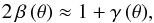 (70)independent of δ, that is valid for the previously mentioned values for δ at smaller radii . It also applies at very large distances
  , since then, the numerical values inside the brackets of Eq. (68) are close to 1 and this equation is fulfilled for any value of the exponents β and γ in all cases. Only for intermediate distances from the star at lower values of δ (not close to 1), the relationship between β and γ is possibly not well approximated by Eq. (70).
2.6.6. Fitting formula for the line acceleration
Thus, we can provide another expression for the line acceleration (in Eq. (39)), now dependent on  and on the parameters , γ (or β equivalently), δ and (by eliminating using Eq. (65)):
 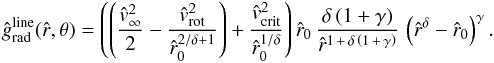 (71)This non-linear expression can then be used as fitting formula and applied to the results from a numerical calculation of
  for discrete radial grid points
  at a given latitude, in order to determine the line acceleration parameters γ (θ) (or equivalently β (θ) by means of Eq. (70)), δ (θ),
  and the terminal velocity
  , cf. Fig. 1.
2.6.7. Physical interpretation of the equation of critical radius
Through the use of the exact wind solution, by using Eq. (42), valid for the critical radius at latitude with polar angle θ, we can solve for the line acceleration parameter ĝ0 and insert it into Eq. (63) from the approximated wind solution, to provide another expression for the terminal velocity at θ, depending on the location of the critical (i.e. sonic) point ![Mathematical equation: \begin{eqnarray} \label{v-inf-rc} {\hat v}_{\infty}\,(\theta) & = & \left[ \frac{2}{\hat r_{0}} \left\{ \left( \frac{ {\hat r}_{\rm c}^{\delta} }{ {\hat r}_{\rm c}^{\delta} - {\hat r_{0}}}\right)^{\gamma} \frac{ {\hat r}_{\rm c}^{\delta \,-\, 2} }{\delta \left( 1+\gamma\right)} \left( {\hat v}_{\rm crit}^{2}\,{\hat r}_{\rm c} - 2\, {\hat r}_{\rm c}^{2} - {\hat v_{\rm rot}}^{2} \right) \phantom{\frac{{\hat v_{\rm rot}}^{2}}{{\hat r_{0}}^{2 / \delta}}} \right. \right. \nonumber\\ & &\left.\qquad\qquad \left. -~ {\hat v}_{\rm crit}^{2} {\hat r_{0}}^{1 \,-\, 1/ \delta} \right\} + \frac{{\hat v_{\rm rot}}^{2}}{{\hat r_{0}}^{2 / \delta}} \right]^{1/2} \cdot \end{eqnarray}](/articles/aa/full_html/2014/04/aa23031-13/aa23031-13-eq260.png) (72)Or vice versa, by Eq. (42), the location of the critical point (through which the exact analytical wind solution of our Eq. of motion EOM (40) passes) is mainly determined, on the one hand, by the given terminal velocity v∞, via the line acceleration parameter . On the other hand, the position of must also be dependent on the given minimum velocity vin (θ) at the inner boundary radius Rin (θ), where the velocity solution passes. This inner velocity vin follows indirectly from the other remaining line acceleration or wind parameters γ, δ (which make up the shape of the velocity curve) and especially (where the value of the latter parameter is determined by the radius
(72)Or vice versa, by Eq. (42), the location of the critical point (through which the exact analytical wind solution of our Eq. of motion EOM (40) passes) is mainly determined, on the one hand, by the given terminal velocity v∞, via the line acceleration parameter . On the other hand, the position of must also be dependent on the given minimum velocity vin (θ) at the inner boundary radius Rin (θ), where the velocity solution passes. This inner velocity vin follows indirectly from the other remaining line acceleration or wind parameters γ, δ (which make up the shape of the velocity curve) and especially (where the value of the latter parameter is determined by the radius  at which
  is zero).
Since the inner boundary condition of the velocity vin (θ) is connected to the mass-loss rate Ṁ (θ), through the equation of mass continuity by Eq. (13) and the given density at the inner boundary, the position of the critical radius is uniquely specified by the values of v∞ (θ) and Ṁ (θ).
3. Numerical methods
3.1. Computing the radiative acceleration
As in Paper I, we first calculate the thermal, density and ionisation structure of the wind model by means of the non-LTE expanding atmosphere (improved Sobolev approximation) code ISA-Wind (de Koter et al. 1993, 1997). As a next step, we calculate the radiative acceleration as a function of distance by means of a Monte Carlo (MC) code MC-Wind (de Koter et al. 1997; Vink et al. 1999), accounting for the possibility that the photons can be scattered or eliminated (if they are scattered back into the star). The radiative transfer in MC-Wind involves multiple continuum and line processes using the Sobolev approximation (cf. Mazzali & Lucy 1993).
The radiative acceleration of the wind at a given constant co-latitude θ is calculated by following the fate of the large number of photons where the atmosphere is divided into a large number of concentric thin shells with radius r and thickness dr, and the loss of photon energy, due to all scatterings that occur within each shell, is determined. The total line acceleration per shell summed over all line scatterings in that shell equals (Abbott & Lucy 1985) 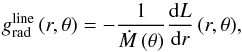 (73)here, (in contrast to the one-dimensional case) referred to a constant polar angle θ, where −dL (r,θ) is the rate at which the radiation field loses energy by the transfer of momentum of the photons to the ions of the wind per time interval.
The line list that is used for the MC calculations consists of over 105 of the strongest lines of the elements from H to Zn from a line list constructed by Kurucz & Bell (1995). Lines in the wavelength region between 50 and 10 000 Å are included with ionisation stages up to stage VII. The number of photon packets distributed over the spectrum in our wind model, followed from the lower boundary of the atmosphere, is 2–3.5 × 10⁷. The wind is divided into 90 spherical shells with a large number of narrow shells in the subsonic region and wider shells in the supersonic range.
3.2. Computing the mass-loss rate for known stellar and wind parameters
By neglecting the pressure term and using the expression for the line acceleration per shell (Eq. (73)), an integration of the Eq. of motion (35) at a given constant latitude, from stellar radius to infinity, yields (cf. Abbott & Lucy 1985) 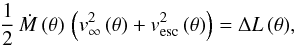 or equivalently,
 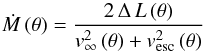 (74)(as in Paper I, but here depending on θ), where ΔL (θ) is the total amount of radiative energy extracted per second, summed over all the shells (at co-latitude θ). This equation is now fundamental for determining mass-loss rates numerically from the total removed radiative luminosity, for the prespecified stellar and wind parameters vesc (θ) and v∞ (θ), respectively.
3.3. The iteration method: determination of  and the wind parameters
To compute the mass-loss rate and the wind model parameters from a given rotating central star with the fixed stellar parameters6L (θ), Teff (θ), R (θ), M, Γ (θ), Vrot, the analogous iterative procedure as in the one-dimensional non-rotating case can be applied (cf. Paper I). However, the whole iteration cycle here has to be performed separately for each given co-latitude θ of interest:
-
1.
By keeping the stellar and wind parametersṀn(θ), v∞n(θ), βn(θ) variable throughout our iteration process, we use arbitrary (but reasonable) starting values Ṁ-1, v∞-1, β-1 in iteration step n = −1 (cf. Tables A.1–A.4).
-
2.
For these input parameters, a model atmosphere is calculated with ISA-Wind for constant co-latitude θ. The code yields the thermal structure, the ionisation and excitation structure, and the population of energy levels of all relevant ions. Then, the radiative acceleration
 is calculated for discrete radial grid points ri at polar angle θ with MC-Wind and Eq. (73). In addition, an improved estimate for the mass-loss rate
  is obtained by Eq. (74), which can be used as a new input value for the next iteration step. Moreover, one obtains a new output value for the sonic radius
  (which has to be equal to the critical radius
  of our wind theory).
 -
3.
To determine the improved line acceleration parameters γn(θ) (or equivalently βn(θ)), δn(θ) and
 for the considered latitude, Eq. (71) (together with Eq. (70)) is used as the fitting formula to apply to the numerical results for , cf. Fig. 1.
 -
4.
By applying Eq. (72) and inserting the current values of parameters γn, δn and
 , as well as the current sonic radius
  for , we obtain a new approximation of the terminal velocity v∞n(θ), i.e.
 ![Mathematical equation: \begin{eqnarray} \label{v-inf-next} v_{{\infty}_{n}}(\theta) & = & a \left[ \frac{2}{\hat r_{{0}_{n}}} \Bigg( \left( \frac{ {\hat r}_{{\rm s}_{n}}^{{\delta}_{n}} }{ {\hat r}_{{\rm s}_{n}}^{{\delta}_{n}} - {\hat r_{{0}_{n}}}}\right)^{\gamma_{n}} \!\!\! \frac{ {\hat r}_{{\rm s}_{n}}^{{\delta_{n}} - 2} }{\delta_{n} \left( 1+\gamma_{n}\right)} \left( {\hat v}_{\rm crit}^{2}\, {\hat r}_{{\rm s}_{n}} \! -\! 2\, {\hat r}_{{\rm s}_{n}}^{2} \!-\! {\hat v}_{\rm rot}^{2}\right) \right.\nonumber\\[2mm] & &\left. - {\hat v}_{\rm crit}^{2} {\hat r_{{0}_{n}}}^{1 - 1/ {\delta_{n}}} \Bigg) + \frac{{\hat v_{\rm rot}}^{2}}{ {\hat r_{{0}_{n}}}^{2 / \delta_{n} }} \right]^{1/2} \cdot \end{eqnarray}](/articles/aa/full_html/2014/04/aa23031-13/aa23031-13-eq301.png) (75)
(75) -
5.
With these improved estimates of Ṁn(θ), v∞n(θ), βn(θ) as new input parameters, the whole iteration step, defined by items 2–4, is repeated until convergence (at given latitude) is achieved.
3.4. The adjustment of the wind formalism to ISA-Wind
The ISA-Wind code has already been described in detail by de Koter et al. (1993, 1996). Those model assumptions within ISA-Wind which affect our wind formalism, by using the code in our iteration process, have also been described in Paper I.
To be able to apply the analytical wind solution of our EOM (40) to model a stellar wind from a given central star (with fixed stellar parameters) by using ISA-Wind to find numerically the unique solution, we had to adjust our wind formalism, i.e. our more accurate EOM, to the assumed EOM and wind velocity structure in ISA-Wind. The EOM (40) (and therefore our exact analytical wind solution) considers (allows) a line acceleration throughout the whole wind regime, starting above the radius  , whereas the different EOM in ISA-Wind is only solved in the subsonic region by neglecting the line force. However then, ISA-Wind “switches on” the line force somewhere below a connection radius
  in the subsonic region by assuming a β velocity law above in the supersonic region.
This inconsistency through the use of ISA-Wind (compared to our model assumptions and solutions) has been eliminated by introducing the parameter  into our formalism of Sect. 2 for which the line radiation force is zero at radius at a given co-latitude θ. Then, the final value of , together with the other remaining line acceleration or wind parameters, can be determined by fitting Eq. (71) and the iteration procedure.
Moreover, a further inconsistency would occur if we applied ISA-Wind, developed for non-rotating spherical winds, in our iteration method to compute the wind parameters from a rotating star: the EOM in ISA-Wind for the subsonic region and the assumed β velocity law for the supersonic wind region, therein, do not consider the additional centrifugal term  in contrast to our more accurate EOM (40), which we solve for the radial wind velocity from rotating stars. Therefore, to compensate for this discrepancy, one has to neglect the centrifugal term in our simplified EOM (59) for the supersonic wind region, which results a simpler approximated wind solution and terminal velocity v∞ (θ) than that in Eq. (62) and Eq. (63), respectively, where
  can be set to zero. Then, this in turn, leads also to a simpler expression for the fitting formula for the line acceleration where the term in Eq. (71) vanishes. However, the derivation of the expression for the terminal velocity v∞ (θ), as a function of critical radius (or sonic radius
  ) in Sect. 2.6.7, yields then almost the same Eq. (72), where only the last
  -term (from the simplified approximated wind solution) vanishes but not the
  -term that originates from our equation of critical radius, Eq. (42). The latter takes the stellar rotational speed
  at co-latitude θ and its influence on the location of the critical point into consideration.
To avoid this inconsistency in our subsequent wind models for rotating O-stars in Sect. 4, we have thus applied the following simplified fitting formula 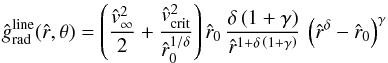 (76)(instead of Eq. (71)) to determine gradually the improved line acceleration parameters by our iterative procedure for a given constant co-latitude θ, whereas the new estimate of the terminal velocity for the next step has been determined by the simplified iteration formula
 ![Mathematical equation: \begin{eqnarray} \label{simpl-v-inf-next} v_{{\infty}_{n}}(\theta) & = & a \left[ \frac{2}{\hat r_{{0}_{n}}} \left( \left( \frac{ {\hat r}_{{\rm s}_{n}}^{{\delta}_{n}} }{ {\hat r}_{{\rm s}_{n}}^{{\delta}_{n}} - {\hat r_{{0}_{n}}}}\right)^{\gamma_{n}} \!\!\! \frac{ {\hat r}_{{\rm s}_{n}}^{{\delta_{n}} - 2} }{\delta_{n} \left( 1+\gamma_{n}\right)} \left( {\hat v}_{\rm crit}^{2}\, {\hat r}_{{\rm s}_{n}} -\, 2\, {\hat r}_{{\rm s}_{n}}^{2} - {\hat v}_{\rm rot}^{2}\right) \right.\right.\nonumber\\[2mm] & & \left.\left. \phantom{ \left( \frac{ {\hat r}_{{\rm s}_{n}}^{{\delta}_{n}} }{ {\hat r}_{{\rm s}_{n}}^{{\delta}_{n}} - {\hat r_{{0}_{n}}}}\right)} - {\hat v}_{\rm crit}^{2} {\hat r_{{0}_{n}}}^{1 - 1/ {\delta_{n}}} \right) \right]^{1/2} , \end{eqnarray}](/articles/aa/full_html/2014/04/aa23031-13/aa23031-13-eq312.png) (77)instead of the generally more accurate Eq. (75).
(77)instead of the generally more accurate Eq. (75).
Stellar and wind parameters for a differentially rotating O5-V main sequence star (with Vrot = 300 km s-1 (Ω = 0.42) and 500 km s-1 (Ω = 0.70), respectively, without distortion) at the pole (θ = 0) and the equator (θ = π/2)a.
Further, since ISA-Wind begins its computations already below (however close to) the stellar (i.e. photospheric) radius, all formulae derived in Sect. 2 have been applied with reference to the inner boundary (core) radius Rin (θ) from where the numerical calculations of the wind model start. Therefore, the dimensionless variable of distance at polar angle θ (in Sect. 4) refers to R = Rin (θ).
3.5. The chosen boundary values in the wind models
In our following numerical wind models the inner boundary radius has been chosen constant throughout the whole iteration process for each chosen latitude and star. E.g., for the particular case of the wind from the undistorted rotating O-main-sequence star (cf. Table 1), it is even constantly Rin =11.757 R⊙ at each co-latitude θ (e.g. at 0 and π/2), situated at a prescribed fixed Rosseland optical depth of about τR = 23. This corresponds then to a photospheric radius of Rphot = 11.828 R⊙ (at each latitude), defined as where the thermal optical depth is  , and an inner boundary density of ρin = 1.398 × 10⁻⁸ g/cm3 at Rin.
Small changes of this particular chosen fixed value for τR, or corresponding ρin (θ), at each step of the iteration cycle (generally dependent on the given co-latitude θ and stellar rotation Vrot in the case of a distorted star, cf. Table 3) would have no effect on the final wind parameters, i.e. in particular on the converged values of Ṁ (θ) and v∞ (θ), as already explained in our 1D Paper I.
4. Application: results for rotating O-stars
In this section we apply our theoretical results from Sect. 2 and the iterative procedure described in Sect. 3.3 to first compute the stellar wind parameters for a differentially rotating 40 M⊙ O5–V main-sequence star with an equatorial rotation speed of Vrot = 300 km s-1 (Ω = 0.42) and 500 km s-1 (Ω = 0.70), respectively. Secondly, we determine the wind parameters for a 60 M⊙ O-giant star rotating with Vrot = 300 km s-1 (Ω = 0.55). In the first instance, we ignore the effects of stellar distortion and gravity darkening in order to be able to compare our procedures against previous models, such as those from FA, before we include the more realistic aspects involving stellar distortion in Sect. 4.2.
4.1. Rotating O-stars without distortion
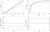 |
Fig. 3 Model results for the wind from a differentially rotating O5–V main-sequence star without distortion with an equatorial rotation speed of Vrot = 300 km s-1 (see dashed curves) and 500 km s-1 (see dotted-dashed curves) at the equator (for θ = π/2), compared to the spherical wind from a corresponding non-rotating star (Vrot = 0) which is identical to the wind from the rotating star at the pole for θ = 0 (see solid curves or solid horizontal lines, respectively); as for the stellar and wind parameters see Table 1 in Sect. 4. All diagrams are plotted vs. radial distance |


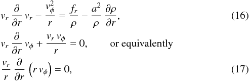
Stellar and wind parameters for a differentially rotating O5-V main sequence star (with Vrot = 300 km s-1 (Ω = 0.70) and 500 km s-1 (Ω = 0.92), respectively) at the pole (θ = 0) and the equator (θ = π/2), considering the stellar distortion and the effects of gravity darkening.
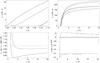 |
Fig. 4 Model results for the wind from a differentially rotating O5–V main-sequence star considering its oblateness including gravity darkening effects with an equatorial rotation speed of Vrot = 300 km s-1 (see dashed curves) and 500 km s-1 (see dotted-dashed curves) at the equator (for θ = π/2), compared to the wind from the pole at θ = 0 (see solid curves or solid horizontal lines, respectively); as for the stellar and wind parameters see Table 3 in Sect. 4. All diagrams are plotted vs. radial distance |
The fixed parameters (see e.g. Martins et al. 2005 and references therein) of the O-main-sequence star are given in the upper part of Table 1, whereas the fixed stellar parameters of the 60 M⊙ O-giant are displayed in the upper part of Table 2. The iteration steps are provided in the Appendix. The final results are listed in the lower part of Tables 1 and 2 respectively, and shown graphically for the OV star in Fig. 3. It can be noted that the predicted mass-loss has barely changed from the spherical case for the model rotating with 300 km s-1. For the more rapidly rotating 500 km s-1 model, the equatorial mass-loss rate increases slightly, by ~0.1 dex, in rough agreement with previous studies, such as FA. Furthermore, the terminal wind velocities also remain relatively constant, although they drop by up to 15% for the most rapid models.
The ratio of equatorial-to-polar density (ρeq/ρp) reaches a constant value at a sufficient distance from the stellar surface, which follows from Eq. (15)  (78)as illustrated, e.g., in the right diagram of Fig. 3 (lower panel). We therefore provide this ratio at infinity in all Tables 1–3.
For the rapid rotator (500 km s-1) with the slightly enhanced equatorial mass-loss rate, we find a density contrast ratio of equator to the pole that varies with stellar distance, has a maximum of about 1.7 close to the star, and then approaches a constant value of ~1.5.
Next we turn our attention to the 60 M⊙ O-giant rotating with Vrot = 300 km s-1. Here we find the effects of rotation to be more pronounced than for the main sequence dwarf. Already at velocities as low as 300 km s-1 the mass-loss rate at the equator is more than a factor two larger than for the spherical non-rotating case, and the equator-to-pole density contrast ratio is (ρeq/ρp)∞ ≃ 2.4.
4.2. Considering oblateness and gravity darkening of the rotating O-main sequence star
We now turn our attention to the physically more realistic cases, including the effects of stellar oblateness and gravity darkening. The model parameter and results are listed in Table 3 and the iteration cycles are shown in the Appendix. Again the results are also shown graphically (in Fig. 4). The situation is notably different from the non-distorted case. Whilst the results for the 300 km s-1 (Ω = 0.70) main-sequence dwarf are inconspicuous as they are not all that different from the spherical case, the behaviour of (ρeq/ρp) again varies somewhat with stellar distance, having its maximum of about 1.25 at about r/R =3.0, and then very slowly decreasing to approach a value of 0.97 at infinity. The more rapid rotator (at 500 km s-1 and Ω = 0.92) shows, seemingly surprisingly, a lower mass-loss rate at the equator than at the pole, by almost an order of magnitude.
The right bottom panel of Fig. 4 also shows the opposite effect: the ratio of equatorial-to-polar density (ρeq/ρp) is significantly below 1, by about a factor of 5. In other words, the predictions including gravity darkening suggest a polarward rather than equatorial stellar wind. How can we understand this result? As can be noted from Eq. (33) the Eddington parameter has become modified to correct for the latitudinal surface distortion. In comparison to the 1D spherical case the luminosity L and effective temperature Teff are lower and using the results of Vink et al. (2000) one can already expect the lowered equatorial mass-loss rate in comparison to the spherical case primarily due to the lower L. These results suggest that for rapid rotators, the big difference between the pole and equator would lead to significantly different diagnostics for a star that is observed from the pole or equator (see e.g. Hillier et al. 2003; Herrero et al. 2012). On a positive note, the pole-to-equator ratio of order 5 is sufficiently large to be measurable with linear polarisation data.
5. Discussion and conclusions
5.1. Comparison with previous models
The earliest works on CAK-type mass-loss predictions including the effects of stellar rotation via the effective mass in the equation of motion (but without considering gravity darkening) such as those by FA and Pauldrach et al. (1986), Petrenz & Puls (2000) resulted in moderate mass-loss rate enhancements, which were subsequently included in evolutionary calculations (Langer 2012). Our results, with mass-loss rates increases by at most 0.1 dex, are in good agreement with these earlier works based on the CAK theory.
When gravity darkening is included, previous studies, such as those of Owocki et al. (1996), Maeder (1999) and Pelupessy et al. (2000) all found relatively modest changes for low rotational velocities, but they all favour polar ejection for high rotation rates in close proximity to the break-up limit (Ω = 1). The most-oft used formulae for mass-loss enhancement on the basis of the CAK theory is the one given by Maeder & Meynet (2000). Their famous equation (4.29) reads: ![Mathematical equation: \begin{equation} \frac{\dot{M}(\Omega)}{\dot{M}(\Omega=0)} = \frac{(1-\Gamma)^{\frac{1}{\alpha}-1}}{\left[ 1-\frac{\Omega^2}{2\pi G \rho_{\rm m}} - \Gamma \right]^{\frac{1}{\alpha}-1}}, \label{EqMdotRot} \end{equation}](/articles/aa/full_html/2014/04/aa23031-13/aa23031-13-eq377.png) (79)where Γ = L/LEdd = κL/(4πcGM) is the Eddington factor (with κ the total opacity), and α the Teff −dependent CAK force multiplier parameter. Whilst it is claimed that the mass-loss increase is due to rotation (Ω) the more relevant reason for the high mass-loss rate is in fact the high Γ factor (see more recent computations by Vink 2006; Gräfener & Hamann 2008; Vink et al. 2011).
(79)where Γ = L/LEdd = κL/(4πcGM) is the Eddington factor (with κ the total opacity), and α the Teff −dependent CAK force multiplier parameter. Whilst it is claimed that the mass-loss increase is due to rotation (Ω) the more relevant reason for the high mass-loss rate is in fact the high Γ factor (see more recent computations by Vink 2006; Gräfener & Hamann 2008; Vink et al. 2011).
Surprisingly, our 2D results that take gravity darkening into account predict a equatorial decrease in the mass-loss rate. This would also imply that the total (cf. Eq. (14)) mass-loss rate is now lower than for the spherical 1D case. This is in contradiction to the above Maeder & Meynet equation that is oftentimes used in stellar evolution calculations for rotating massive stars.
5.2. Comparison with observations
There are two complementary types of astronomical techniques that can provide meaningful geometric constraints on large-scale 2D wind structures. These are interferometry and linear spectropolarimetry. The current status is that whilst interferometry has been very successful in obtaining results on objects such as classical Be stars, B[e] supergiants, and LBVs, results for O stars are – to the best of our knowledge – not yet available due to their smaller radii.
Linear spectropolarimetry can be employed with at least two levels of complexity. The first involves detailed line-profile predictions that can be used to determine the geometric and kinematic environments around young and massive stars (Harries 2000; Vink et al. 2005), as well as the polarimetric agents (Kuhn et al. 2007). The lower-level complexity application of linear spectropolarimetry is adopted here, with the emission line reasonably assumed to be unpolarised, but with the continuum responsible for the observed polarisation level: depolarisation (Poeckert & Marlborough 1976; Brown & McLean 1977). This latter approach is sufficient for our current comparisons. In this case a pole-to-equator density contrast of 5 might lead to a continuum polarisation of ≃1% according to the expectations of Harries et al. (1998).
If we assume that our most realistic density-contrast predictions concern those models that include gravity darkening, we would anticipate the vast majority of mostly moderately rotating O-dwarfs to be unpolarised, as the density contrast between the pole and equator is close to unity for rotation velocities up to 300 km s-1. These overall findings are in good agreement with the linear Hα polarimetry survey of Vink et al. (2009).
An exception might involve the sub-group of Oe stars, for which Vink et al. (2009) list the highest rotation velocities, with vsini values approaching ≃400 km s-1. As this concerns a lower limit (due to the inclination effects), the true rotational velocities of Oe stars might go all the way up to the break-up limit (Ω = 1). Interestingly, the Oe star HD 45314 was indeed shown to have a line effect, but the overall incidence of line effects in Oe stars was low: 1/6. On the basis of the general spectroscopic similarity between Oe and Be stars, and the presence of double-peaked line profiles many astronomers would expect Oe stars to be embedded in circumstellar disks, although it should be noted that spectroscopy alone cannot provide geometric constraints, without complementary imaging, interferometry, or polarimetry, because geometric information from spectral line profiles is not unique, due to the convolution that underlies spectral line formation. In particular, double-peaked profiles can even be noted in spherical shells (e.g. PP).
In the current paper the surprising result is that of polar outflows, whilst it should be noted that linear spectropolarimetry cannot yet distinguish between a prolate (polar) or oblate (equatorial) wind structure (e.g. Wood et al. 1997). It will be challenging to reconcile our axisymmetric density-contrast predictions with the general expectation that Oe/Be stars are embedded within equatorial structures. Clearly there are many puzzles remaining in the geometry and formation of circumstellar media around rotating OB stars, and quite possibly additional physical effects, such as magnetic fields, pulsations, and companions may need to be considered.
5.3. Summary and future work
In Paper I (Müller & Vink 2008), we proposed a new parametrisation of the radiative line acceleration, expressing it as a function of radius rather than of the velocity gradient (as in CAK theory) which generalised the classical thermal Parker (1958) wind and allowed solving it analytically. This has the advantage of higher accuracy and enables to check an influence of numerical viscosity if used as a test example for numerical simulations. In addition, the implementation of this formalism allows for local dynamical consistency as we are able to determine the momentum transfer at each location in the wind through the use of Monte Carlo simulations.
In this paper, we present a generalization of our model of spherical line-driven winds (in Paper I) to the case of axially symmetric rotating stars. We extend on the results of Paper I, deriving analytical solutions for the 2D case in an axisymmetric mass outflow or inflow scenario. The generalization approximates the solution of the two-dimensional problem of a rotating wind as a one-parametric set (parameterised by the latitude) of one-dimensional solutions. Here, the separation of the radial motion for individual latitudes is achieved by the basic assumption that the meridional flow velocity is negligible. Assuming furthermore only central external forces, then imply the conservation of angular momentum and leads to an additional centrifugal term in the equation of radial motion7. We also extend our iterative method for the simultaneous solution of the mass-loss rate and velocity field to the case of a rotating non-spherical stellar wind, using the parameterised description of the line acceleration that only depends on radius – at any given latitude.
Furthermore, an approximate analytical solution for the supersonic flow of a rotating wind is derived, which closely resembles the exact solution, and we apply the new expressions with our iterative method to (i) the stellar wind from a differentially rotating 40 M⊙ O5–V main sequence star; as well as to (ii) a 60 M⊙ O-giant star. We subsequently account for the effects of stellar oblateness and gravity darkening for the O5–V main sequence star. The results show an equatorial decrease in the mass-loss rate, which would imply a total mass-loss rate that is lower than for the spherical 1D case, in contradiction to the oft-used Maeder & Meynet (2000) formalism used in most current stellar evolution calculations for rotating massive stars.
In the future we plan to extend our method to B supergiants, in particular to tackle the problem of disk-formation in B[e] supergiants (Lamers & Pauldrach 1991; Pelupessy et al. 2000; Cure et al. 2005; Madura et al. 2007).
Online material
Appendix A: Tables of iteration cycles
Iteration cycles for the equatorial wind from a rotating O5–V main-sequence star with Vrot = 300 km s-1 (see upper table) and Vrot = 500 km s-1 (see lower table) without distortion.
Iteration cycles for the wind from an O-giant star rotating with Vrot = 300 km s-1 at the pole (see upper table) and at the equator (see lower table) without distortion.
Iteration cycles for the wind from a rotating O5–V main-sequence star with Vrot = 300 km s-1 at the pole (see upper table) and at the equator (see lower tables) considering the stellar distortion and the effects of gravity darkening.
Iteration cycles for the wind from a rotating O5–V main-sequence star with Vrot = 500 km s-1 at the pole (see upper table) and at the equator (see middle and lower tables) considering the stellar distortion and the effects of gravity darkening.
We are here not interested in the presentation of the polar vector eθ, because the velocity component vθ will be later set to zero.
...as, e.g., most stellar wind models from early-type massive stars adopt (e.g. CAK, FA, BC). However, it should be noted that this restricting assumption of an absent friction excludes the transport of angular momentum in a disk, which is mostly dominant in the case of a collapsing system with accretion.
The adjustment of our analytical expressions (for the wind solution) to the non-isothermal model wind is here achieved by deriving an approximated analytical solution for the supersonic wind regime, which introduces a terminal velocity v∞ to our initially assumed isothermal wind, and provides a relationship between v∞ and our wind solution parameters (cf. explanations in Paper I, Sects. 2.5.4. and 2.5.9.).
Nevertheless, Gayley & Owocki (2000) show how even in a wind that is azimuthally symmetric, a net azimuthal line force may result.
We furthermore assume that both and ( ) are everywhere single-valued and continuous.
The centrifugal term was also included by Friend & Castor (1982) in an opposite approximation of an extreme transport of angular momentum able to ensure purely radial motion in a co-rotating frame.
Acknowledgments
We acknowledge financial report from the STFC and DCAL. We thank our anonymous referee for helpful comments.
References
- Abbott, D. C., & Lucy, L. B. 1985, ApJ, 288, 679 [NASA ADS] [CrossRef] [Google Scholar]
- Bjorkman, J. E., & Cassinelli, J. P. 1993, ApJ, 409, 429 [NASA ADS] [CrossRef] [Google Scholar]
- Brown, J. C., & McLean, I. S. 1977, A&A, 57, 141 [NASA ADS] [Google Scholar]
- Castor, J. I., & Lamers, H. J. G. L. M. 1979, ApJS, 39, 481 [NASA ADS] [CrossRef] [Google Scholar]
- Castor, J. I., Abbott, D. C., & Klein, R. I. 1975, ApJ, 195, 157 [NASA ADS] [CrossRef] [Google Scholar]
- Collins, G. W. 1965, ApJ, 142, 265 [NASA ADS] [CrossRef] [Google Scholar]
- Corless, R. M., Gonnet, G. H., Hare, D. E. G., & Jeffrey, D. J. 1993, Maple Technical Newsletter, 9, 12 [Google Scholar]
- Corless, R. M., Gonnet, G. H., Hare, D. E. G., Jeffrey, D. J., & Knuth, D. E, 1996, Adv. Comput. Math., 5, 329 [CrossRef] [MathSciNet] [Google Scholar]
- Cranmer, S. R., & Owocki, S. P. 1995, ApJ, 440, 308 [NASA ADS] [CrossRef] [Google Scholar]
- Cure, M., Rial, D. F., & Cidale, L. 2005, A&A, 437, 929 [NASA ADS] [CrossRef] [EDP Sciences] [Google Scholar]
- de Koter, A., Schmutz, W., & Lamers, H. J. G. L. M. 1993, A&A, 277, 561 [NASA ADS] [Google Scholar]
- de Koter, A., Lamers, H. J. G. L. M., & Schmutz, W. 1996, A&A, 306, 501 [NASA ADS] [Google Scholar]
- de Koter, A., Heap, S. R., & Hubeny, I. 1997, ApJ, 477, 792 [Google Scholar]
- Espinosa Lara, F., & Rieutord, M. 2013, A&A, 552, A35 [NASA ADS] [CrossRef] [EDP Sciences] [Google Scholar]
- Friend, D. B., & Abbott, D. C. 1986, ApJ, 311, 701 [NASA ADS] [CrossRef] [Google Scholar]
- Friend, D. B., & Castor, J. I. 1982, ApJ, 261, 293 [NASA ADS] [CrossRef] [Google Scholar]
- Gayley, K. G., & Owocki, S. P. 2000, ApJ, 537, 461 [NASA ADS] [CrossRef] [Google Scholar]
- Gräfener, G., & Hamann, W.-R. 2008, A&A, 482, 945 [NASA ADS] [CrossRef] [EDP Sciences] [Google Scholar]
- Groh, J. H., Hillier, D. J., & Damineli, A. 2006, ApJ, 638, 33 [Google Scholar]
- Harries, T. J. 2000, MNRAS 315, 722 [Google Scholar]
- Harries, T. J., Hillier, D. J., & Howarth, I. D. 1998, MNRAS 296, 1072 [Google Scholar]
- Harries, T. J., Howarth, I. D., & Evans, C. J. 2002, MNRAS 337, 341 [Google Scholar]
- Herrero, A., Garcia, M., Puls, J., et al. 2012, A&A, 543, A85 [NASA ADS] [CrossRef] [EDP Sciences] [Google Scholar]
- Hillier, D. J., Lanz, T., Heap, S. R., et al. 2003, ApJ, 588, 1039 [NASA ADS] [CrossRef] [Google Scholar]
- Hoffman, J. L., Leonard, D. C., Chornock, R., et al. 2008, ApJ, 688, 1186 [NASA ADS] [CrossRef] [Google Scholar]
- Kuhn, J. R., Berdyugina, S. V., Fluri, D. M., Harrington, D. M., & Stenflo, J. O. 2007, ApJ, 668, 63 [NASA ADS] [CrossRef] [Google Scholar]
- Kurucz, R. L., & Bell, B. 1995, Atomic line list, Kurucz CD-ROM (Cambridge, MA: Smithsonian Astrophysical Observatory) [Google Scholar]
- Lamers, H. J. G. L. M., & Pauldrach, A. W. A. 1991, A&A, 244, 5 [Google Scholar]
- Langer, N. 2012, ARA&A, 50, 107 [NASA ADS] [CrossRef] [Google Scholar]
- Lovekin, C. C. 2011, MNRAS, 415, 3887 [NASA ADS] [CrossRef] [Google Scholar]
- Madura, T. I., Owocki, S. P., & Feldmeier, A. 2007, ApJ, 660, 687 [NASA ADS] [CrossRef] [Google Scholar]
- Maeder, A. 1999, A&A, 347, 185 [NASA ADS] [Google Scholar]
- Maeder, A., & Meynet, G. 2000, A&A, 361, 159 [NASA ADS] [Google Scholar]
- Maeder, A., & Meynet, G. 2012, Rev. Mod. Phys., 84, 25 [NASA ADS] [CrossRef] [Google Scholar]
- Meynet, G., & Maeder, A. 2007, A&A, 464, 11 [Google Scholar]
- Martins, F., Schaerer, D., & Hillier, D. J. 2005, A&A, 436, 1049 [NASA ADS] [CrossRef] [EDP Sciences] [Google Scholar]
- Maund, J. R., Wheeler, J. C., Patat, F., et al. 2007, ApJ, 671, 1944 [NASA ADS] [CrossRef] [Google Scholar]
- Mazzali, P. A., & Lucy, L. B. 1993, A&A, 279, 447 [NASA ADS] [Google Scholar]
- Mihalas, D., & Weibel Mihalas, B. 1984, Foundations of Radiation Hydrodynamics (Oxford: University Press) [Google Scholar]
- Muijres, L. E., Vink, J. S., de Koter, A., Müller, P. E., & Langer, N. 2012, A&A, 537, A37 [NASA ADS] [CrossRef] [EDP Sciences] [Google Scholar]
- Müller, P. E., & Vink, J. S. 2008, A&A, 492, 493 (Paper I) [NASA ADS] [CrossRef] [EDP Sciences] [Google Scholar]
- Owocki, S. P., Cranmer, S. R., & Gayley, K. G. 1996, ApJ, 472, 115 [Google Scholar]
- Parker, E. N. 1958, ApJ, 128, 664 [Google Scholar]
- Pauldrach, A., Puls, J., & Kudritzki, R. P. 1986, A&A, 164, 86 [NASA ADS] [Google Scholar]
- Pelupessy, I., Lamers, H. J. G. L. M., & Vink, J. S. 2000, A&A, 359, 695 [NASA ADS] [Google Scholar]
- Petrenz, P., & Puls, J. 1996, A&A, 312, 195 [NASA ADS] [Google Scholar]
- Petrenz, P., & Puls, J. 2000, A&A, 358, 956 [NASA ADS] [Google Scholar]
- Poe, C. H. 1987, Ph.D. Thesis, Univ. Wisconsin [Google Scholar]
- Poeckert, R., & Marlborough, J. M. 1976, ApJ, 206, 182 [NASA ADS] [CrossRef] [Google Scholar]
- Porter, J. M., & Rivinius, T. 2003, PASP, 115, 1153 [NASA ADS] [CrossRef] [Google Scholar]
- Puls, J., Vink, J. S., & Najarro, F. 2008, A&ARv, 16, 209 [NASA ADS] [CrossRef] [EDP Sciences] [Google Scholar]
- Vink, J. S. 2006, ASP Conf. Ser., 353, 113 [NASA ADS] [Google Scholar]
- Vink, J. S., de Koter, A., & Lamers, H. J. G. L. M. 1999, A&A, 350, 181 [NASA ADS] [Google Scholar]
- Vink, J. S., de Koter, A., & Lamers, H. J. G. L. M. 2000, A&A, 362, 295 [NASA ADS] [Google Scholar]
- Vink, J. S., Harries, T. J., & Drew, J. E. 2005, A&A, 430, 213 [NASA ADS] [CrossRef] [EDP Sciences] [Google Scholar]
- Vink, J. S., Davies, B., Harries, T. J., Oudmaijer, R. D., & Walborn, N. R. 2009, A&A, 505, 743 [NASA ADS] [CrossRef] [EDP Sciences] [Google Scholar]
- Vink, J. S., Brott, I., Gräfener, G., et al. 2010, A&A, 512, A7 [Google Scholar]
- Vink, J. S., Muijres, L. E., Anthonisse, B., et al. 2011, A&A, 531, A132 [NASA ADS] [CrossRef] [EDP Sciences] [Google Scholar]
- Wood, K., Bjorkman, K. S., & Bjorkman, J. E. 1997, ApJ, 477, 926 [NASA ADS] [CrossRef] [Google Scholar]
- von Zeipel, H. 1924, MNRAS, 84, 665 [NASA ADS] [CrossRef] [Google Scholar]
- Zickgraf, F.-J., Wolf, B., Stahl, O., Leitherer, C., & Klare, G. 1985, A&A, 143, 421 [NASA ADS] [Google Scholar]
All Tables
Stellar and wind parameters for a differentially rotating O5-V main sequence star (with Vrot = 300 km s-1 (Ω = 0.42) and 500 km s-1 (Ω = 0.70), respectively, without distortion) at the pole (θ = 0) and the equator (θ = π/2)a.
Stellar and wind parameters for a differentially rotating O5-V main sequence star (with Vrot = 300 km s-1 (Ω = 0.70) and 500 km s-1 (Ω = 0.92), respectively) at the pole (θ = 0) and the equator (θ = π/2), considering the stellar distortion and the effects of gravity darkening.
Iteration cycles for the equatorial wind from a rotating O5–V main-sequence star with Vrot = 300 km s-1 (see upper table) and Vrot = 500 km s-1 (see lower table) without distortion.
Iteration cycles for the wind from an O-giant star rotating with Vrot = 300 km s-1 at the pole (see upper table) and at the equator (see lower table) without distortion.
Iteration cycles for the wind from a rotating O5–V main-sequence star with Vrot = 300 km s-1 at the pole (see upper table) and at the equator (see lower tables) considering the stellar distortion and the effects of gravity darkening.
Iteration cycles for the wind from a rotating O5–V main-sequence star with Vrot = 500 km s-1 at the pole (see upper table) and at the equator (see middle and lower tables) considering the stellar distortion and the effects of gravity darkening.
All Figures
|
Fig. 1 Dimensionless radiative line acceleration |
| In the text | |
|
Fig. 2 Topology of solutions |
| In the text | |
|
Fig. 3 Model results for the wind from a differentially rotating O5–V main-sequence star without distortion with an equatorial rotation speed of Vrot = 300 km s-1 (see dashed curves) and 500 km s-1 (see dotted-dashed curves) at the equator (for θ = π/2), compared to the spherical wind from a corresponding non-rotating star (Vrot = 0) which is identical to the wind from the rotating star at the pole for θ = 0 (see solid curves or solid horizontal lines, respectively); as for the stellar and wind parameters see Table 1 in Sect. 4. All diagrams are plotted vs. radial distance |
| In the text | |
|
Fig. 4 Model results for the wind from a differentially rotating O5–V main-sequence star considering its oblateness including gravity darkening effects with an equatorial rotation speed of Vrot = 300 km s-1 (see dashed curves) and 500 km s-1 (see dotted-dashed curves) at the equator (for θ = π/2), compared to the wind from the pole at θ = 0 (see solid curves or solid horizontal lines, respectively); as for the stellar and wind parameters see Table 3 in Sect. 4. All diagrams are plotted vs. radial distance |
| In the text | |
Current usage metrics show cumulative count of Article Views (full-text article views including HTML views, PDF and ePub downloads, according to the available data) and Abstracts Views on Vision4Press platform.
Data correspond to usage on the plateform after 2015. The current usage metrics is available 48-96 hours after online publication and is updated daily on week days.
Initial download of the metrics may take a while.