| Issue |
A&A
Volume 658, February 2022
|
|
|---|---|---|
| Article Number | A194 | |
| Number of page(s) | 33 | |
| Section | Stellar atmospheres | |
| DOI | https://doi.org/10.1051/0004-6361/202141920 | |
| Published online | 24 February 2022 | |
Metallicities in M dwarfs: Investigating different determination techniques★
1
Hamburger Sternwarte,
Gojenbergsweg 112,
21029
Hamburg,
Germany
e-mail: This email address is being protected from spambots. You need JavaScript enabled to view it.
2
Homer L. Dodge Department of Physics and Astronomy, University of Oklahoma,
440 West Brooks Street,
Norman,
OK
73019,
USA
3
Departamento de Construcción e Ingeniería de Fabricación, Universidad de Oviedo, c/ Pedro Puig Adam, Sede Departamental Oeste,
Módulo 7, 1 a planta,
33203
Gijón,
Spain
4
Departamento de Ingeniería de Organización, Administración de Empresas y Estadística, Universidad Politécnica de Madrid,
c/ José Gutiérrez Abascal 2,
28006
Madrid,
Spain
5
Instituto de Astrofísica e Ciências do Espaço, Universidade do Porto, CAUP, Rua das Estrelas,
4150-762
Porto,
Portugal
6
Departamento de Física e Astronomia, Faculdade de Ciências, Universidade do Porto, Rua do Campo Alegre,
4169-007
Porto,
Portugal
7
Departamento de Física de la Tierra y Astrofísica and IPARCOS-UCM (Instituto de Física de Partículas y del Cosmos de la UCM), Facultad de Ciencias Físicas, Universidad Complutense de Madrid,
28040
Madrid,
Spain
8
Centro de Astrobiología (CSIC-INTA), ESAC,
Camino Bajo del Castillo s/n, 28691, Villanueva de la Cañada,
Madrid,
Spain
9
Instituto de Astrofísica de Andalucía (IAA-CSIC),
Glorieta de la Astronomía s/n,
18008
Granada,
Spain
10
Instituto de Alta Investigación, Universidad de Tarapacá,
Casilla 7D,
Arica,
Chile
11
Centro de Astrobiología (CSIC-INTA),
Carretera de Ajalvir km 4,
Torrejón de Ardoz,
28850,
Madrid,
Spain
12
Instituto de Astrofísica de Canarias,
c/ Vía Láctea s/n,
38205
La Laguna,
Tenerife,
Spain
13
Departamento de Astrofísica, Universidad de La Laguna,
38206
La Laguna,
Tenerife,
Spain
14
Thüringer Landessternwarte Tautenburg,
Sternwarte 5,
07778
Tautenburg,
Germany
15
Max-Planck-Institut für Astronomie,
Königstuhl 17,
69117
Heidelberg,
Germany
16
Centro Astronómico Hispano-Alemán (CSIC-MPG), Observatorio Astronómico de Calar Alto,
Sierra de los Filabres, 04550 Gérgal,
Almería,
Spain
17
Landessternwarte, Zentrum für Astronomie der Universität Heidelberg,
Königstuhl 12,
69117
Heidelberg,
Germany
18
Institut für Astrophysik, Georg-August-Universität,
Friedrich-Hund-Platz 1,
37077
Göttingen,
Germany
19
Institut de Ciències de l’Espai (CSIC-IEEC), Campus UAB,
c/ de Can Magrans s/n, 08193 Bellaterra,
Barcelona,
Spain
20
Institut d’Estudis Espacials de Catalunya (IEEC),
08034
Barcelona,
Spain
Received:
30
July
2021
Accepted:
16
November
2021
Abstract
Deriving metallicities for solar-like stars follows well-established methods, but for cooler stars such as M dwarfs, the determination is much more complicated due to forests of molecular lines that are present. Several methods have been developed in recent years to determine accurate stellar parameters for these cool stars (Teff ≲ 4000 K). However, significant differences can be found at times when comparing metallicities for the same star derived using different methods. In this work, we determine the effective temperatures, surface gravities, and metallicities of 18 well-studied M dwarfs observed with the CARMENES high-resolution spectrograph following different approaches, including synthetic spectral fitting, analysis of pseudo-equivalent widths, and machine learning. We analyzed the discrepancies in the derived stellar parameters, including metallicity, in several analysis runs. Our goal is to minimize these discrepancies and find stellar parameters that are more consistent with the literature values. We attempted to achieve this consistency by standardizing the most commonly used components, such as wavelength ranges, synthetic model spectra, continuum normalization methods, and stellar parameters. We conclude that although such modifications work quite well for hotter main-sequence stars, they do not improve the consistency in stellar parameters for M dwarfs, leading to mean deviations of around 50–200 K in temperature and 0.1–0.3 dex in metallicity. In particular, M dwarfs are much more complex and a standardization of the aforementioned components cannot be considered as a straightforward recipe for bringing consistency to the derived parameters. Further in-depth investigations of the employed methods would be necessary in order to identify and correct for the discrepancies that remain.
Key words: methods: data analysis / techniques: spectroscopic / stars: fundamental parameters / stars: late-type / stars: low-mass
Full Tables C.1 and C.2 are only available at the CDS via anonymous ftp to cdsarc.u-strasbg.fr (130.79.128.5) or via http://cdsarc.u-strasbg.fr/viz-bin/cat/J/A+A/658/A194
© ESO 2022
1 Introduction
Precise stellar metallicity determinations are an essential step to achieving a fuller understanding of the dynamical and chemical evolution of the Galaxy. Several methods have been developed to study element abundances of all kinds of stars. Among these, M dwarfs are the most prevalent type in our Galaxy (Henry et al. 2016; Reylé et al. 2021) and therefore an accurate determination of their abundances is of utmost interest. In the fast-growing field of exoplanet detection and characterization, abundance determinations of the host star are also important to better understand the formation and evolution of planetary systems (e.g., Burn et al. 2021).
A popular method for deriving the metallicities of M dwarfs is based on the measurement of pseudo-equivalent widths (pEWs) of spectral lines. This method was used by Neves et al. (2013, 2014), Mann et al. (2013a, 2014), Newton et al. (2014), Maldonado et al. (2015), and Khata et al. (2020), among others. Another widely used approach is spectral synthesis, where the stellar spectrum is synthesized using stellar atmosphere models along with radiative transfer codes and atomic and molecular line lists. The PHOENIX stellar atmosphere code (Hauschildt 1992, 1993) is the basis for stellar model grids such as the BT-Settl model atmospheres (Allard et al. 2012, 2013) and the PHOENIX-ACES synthetic model grid (Husser et al. 2013).
Marfil et al. (2021) used the BT-Settl model atmospheres and the radiative transfer code turbospectrum (Plez 2012) to generate synthetic spectra around 75 Fe I and Ti I lines, along with the TiO γ and ϵ bands, to determine Teff, log g, and [Fe/H] for 342 M dwarfs from the CARMENES survey by means of the SteParSyn code (Tabernero et al. 2018, 2021). The turbospectrum code was also employed by Souto et al. (2017, 2020) and Sarmento et al. (2021), together with 1-D MARCS stellar atmospheres (Gustafsson et al. 2008), to derive stellar parameters and abundances for several M dwarfs observed with the Apache Point Observatory Galactic Evolution Experiment (APOGEE, Majewski et al. 2017). Operating in a wavelength range from 15000 Å to 17000 Å and with high-resolution ( ; Wilson et al. 2010), APOGEE is dedicated to observing red giants, but it has additionally observed around 2000 M dwarfs. Önehag et al. (2012) and Lindgren et al. (2016) fitted synthetic spectra to high-resolution CRIRES J-band spectra of M dwarfs using the Spectroscopy Made Easy package (SME, Valenti & Piskunov 1996; Valenti & Fischer 2005) with MARCS atmospheres. SME computes synthetic spectra on the fly and determines the best fit stellar parameters by χ2 -minimization with the observed spectra. Passegger et al. (2018) fitted the PHOENIX-ACES model spectra grid to high-resolution CARMENES spectra of 300 M dwarfs and derived Teff, log g, and [Fe/H].
Over the last several years, machine learning has emerged as a valuable tool for predicting stellar parameters for large sets of stars. Several applications of neural networks in stellar parameter determination can be found in Fabbro et al. (2018), Birky et al. (2020), Antoniadis-Karnavas et al. (2020), and Passegger et al. (2020), among others. For a more detailed overview on previous works on stellar parameter determinations in M dwarfs, we refer to the literature summaries in Passegger et al. (2020) and Marfil et al. (2021).
It is known from previous stellar parameter studies that different determination methods sometimes provide significantly different results for the same stars. This is shown in the comparison plots of several parameter determination studies, for instance, Fig. 13 in Rojas-Ayala et al. (2012), Figs. 13, 14 in Neves et al. (2014), Figs. 1 and 5 in Lindgren et al. (2016), Figs. 5–7 in Passegger et al. (2019), Fig. 7 in Passegger et al. (2020), Figs. 10–12 in Marfil et al. (2020), Figs. 12 and 13 in Sarmento et al. (2021), and Figs. 9, 11, as well as A1–A6 in Marfil et al. (2021). These inconsistencies challenge the reliability of the determined stellar parameters for the lowest-mass stars.
However, there are different types of inconsistencies. The most relevant cases in this context are inconsistencies between different methods and between different observations of the same star with different instruments. Since there is no way yet to measure the absolute correct physical and atmospheric properties of a given star, we have to rely on the parameters that different methods and observations provide. Deriving consistent values for the same star with different methods (or different instruments) can therefore be considered as a proxy for the reliability of the value of the stellar parameters and of the methods themselves.
Several studies have conducted such consistency analyses for FGK-type stars and examined the differences introduced when deriving abundances with different methods. For example, Hinkel et al. (2016) investigated four G-type stars with high-resolution MIKE spectra ( ) from the Magellan Planet Search Program, with an average signal-to-noise ratio (S/N) of 200, and covering the wavelength range of 5050–7100 Å. Six different teams participated in the analysis and determined abundances for ten elements (C, O, Na, Mg, Al, Si, Fe, Ni, Ba, and Eu), in four different runs. In Run 1, each group used their individual techniques, while in Run 2 standard stellar parameters for Teff, log g, and microturbulent velocity ξ were provided. Run 3 included a standard line list, whereas Run 4 was a combination between Runs 2 and 3. The authors found that Run 2 gave consistently better results between the elements, followed by Run 4, which suggests that stellar parameters other than abundances or line lists should be standardized in order to produce similar results.
A larger sample of 34 Gaia benchmark FGK-type stars was used by Jofré et al. (2014). The spectra were collected with HARPS ( ), NARVAL (
 ), and UVES (
 ), covering a spectral range from 4760 Å to 6840 Å. Seven different teams participated in this study and derived Fe abundances in three runs. Their main aim was to analyze the effects of instrumental resolution on the determination of metallicity when fixing Teff and log g to independently derived values. Furthermore, all teams used a common line list and the same atomic data (see Heiter et al. 2021) and atmosphericmodels (MARCS). In the different runs, they used spectra with their original resolution and with resolution downgraded to
  to study instrumental effects. They found that different resolutions result in a metallicity difference of less than 0.05 dex, and that metallicities agree when using different instruments. A comparison of the different methods showed larger standard deviations in metallicity for the coolest stars (0.1 dex, Teff < 5000 K) than for the hottest stars (0.07 dex, Teff > 5000 K). A follow-up study by Jofré et al. (2015) analyzed ten different element abundances with eight methods taking into account non-local thermodynamical equilibrium (NLTE) corrections for Fe and errors of the fixed stellar parameters. They performed a detail analysis of systematic errors for differential and absolute abundances. For an extensive discussion on each element and NLTE effects, we refer to Jofré et al. (2015).
Jofré et al. (2017) provided a detailed study of four Gaia benchmark stars, the Sun (G2 V), Arcturus (K1.5 III), 61 Cyg A (K5 V), and HD 22879 (G0 V). Their high-resolution spectra from NARVAL and HARPS were convolved to a common resolution of 70,000. Also in this work, the stellar parameters Teff, log g, micro-turbulence vmic, and vsini were fixed for each star. The analysis was performed by six different teams in eight different runs, including tests regarding continuum normalization, common line lists, hyperfine structure, α-enhancement, and radiative transfer code. They concluded that the most important point for consistent metallicity values is a common continuum flux.
Focusing on cooler stars, Slumstrup et al. (2019) conducted a similar study for red giant stars in the open clusters NGC 6819, M67, and NGC 188. They compared several combinations of line lists and methods to derive EWs, and analyzed the systematic uncertainties from a line-by-line spectroscopic analysis. As a result, they found scatter of around 170 K in Teff, 0.4 dex in log g, and 0.25 dex in metallicity, concluding that even for high-precision spectroscopic analyses, external constraints are necessary to obtain consistent results between different methods.
Up to now, no such analysis has been performed for M dwarfs. In this work, we aim to follow the approach by Hinkel et al. (2016) to study the deviations in metallicity, as well as Teff and log g, coming from different determination methods, and to identify ways to derive more consistent results for stars at the cool end of the main sequence. This paper is structured as follows. Section 2 gives an overview on the methods we used in our analyses. Section 3 explains our sample of benchmark stars and the different analysis runs we performed. In Sect. 4, we present the results of the investigation, followed by a discussion in Sect. 5. A short summary is given in Sect. 6.
2 Methods
In the following we describe the four different methods we use for deriving fundamental stellar parameters Teff, log g, and [Fe/H].
2.1 Synthetic spectra fitting
2.1.1 Pass19-code
This method is fully described in Passegger et al. (2018, 2019), hereafter referred to as Pass19-code. We used a downhill simplex method with a χ2 minimization to find the synthetic model spectrum that best fits the observed spectrum by fitting several wavelength ranges in the VIS and NIR simultaneously (see Table 2 in Passegger et al. 2019).
The PHOENIX-ACES model spectra grid (Husser et al. 2013) incorporated here is based on the PHOENIX code developed by Hauschildt (1992, 1993). Improvements to the code are described in Hauschildt et al. (1997), Hauschildt & Baron (1999), Claret et al. (2012), and Husser et al. (2013), for instance. The one-dimensional (1D) mode of the PHOENIX code computes spherically symmetric model atmospheres, which can be used to simulate main sequence stars and brown dwarfs, including L and T spectral types, as well as white dwarfs and giants. It also includes models for expanding envelopes of novae and supernovae, and accretion disks. PHOENIX can calculate synthetic spectra in 1D or 3D and can be executed in LTE or non-LTE radiative transfer mode. Several model atmosphere grids for late-type stars are based on the PHOENIX code, for instance the NextGen models (Hauschildt et al. 1999), the AMES models (Allard et al. 2001), and the BT-Settl models (Allard et al. 2011). For the calculation of the aforementioned PHOENIX-ACES model spectra grid a new equation of state was used, which was especially designed for the formation of molecules invery cool stellar atmospheres. The grid takes into account solar chemical compositions from Asplund et al. (2009), updated with meteoritic values from Lodders et al. (2009). Since the PHOENIX-ACES grid we use has [α/Fe] = 0, our metallicity results of [M/H] directly translate into identical [Fe/H] values. However, for certain parameter ranges, an α-enhanced PHOENIX-ACES grid is available (see Husser et al. 2013).
To match the instrumental resolution and wavelength grid of observed spectra, the PHOENIX-ACES model spectra are convolved with a Gaussian and linearly interpolated in wavelength. The synthetic spectra are broadened to account for the rotational velocity v sin i of the star (Reiners et al. 2018). Therefore, a separate function estimates the effect on the line spread function and the synthetic spectrum is convolved with the resulting line spread function. The pseudo-continuum of both the observed and synthetic spectra is normalized with a linear fit within each small wavelength region that is analyzed.
The surface gravity (log g) is determined from evolutionary models as in Passegger et al. (2019). This is done to break degeneracies between the parameters. The evolutionary models used in this work were taken from the PARSEC v1.2S library (Bressan et al. 2012; Chen et al. 2014, 2015; Tang et al. 2014), which provides Teff and log g for metallicities in the range −2.2 < [M/H] < +0.7 and different stellar ages, among other parameters. To select the appropriate isochrone, we took the stellar ages from Passegger et al. (2019). The log g is then calculated from this isochrone’s Teff – log g relation depending on Teff and [Fe/H] chosen by our algorithm. To get finer values we linearly interpolate for metallicities between −1.0 and +0.7. The PHOENIX-ACES model spectra grid is then interpolated according to these three parameters and the χ2 is calculated between the observed and synthetic spectrum. A downhill simplex finds the best fitting synthetic spectrum with the smallest χ2 by exploring the 2-D Teff-[Fe/H] parameter space and adjusting those parameters accordingly.
2.1.2 SteParSyn
The SteParSyn code is described in detail in Tabernero et al. (2022). It is a Bayesian implementation of the spectral synthesis technique that determines the probability distributions of the stellar atmospheric parameters (Teff, log g, [Fe/H], v sin i, and ζ) from a Markov chain Monte Carlo (MCMC) approach. In general terms, the code compares a grid of synthetic spectra pre-computed around certain spectral features of interest. Therefore, we used a selection of 75 magnetically insensitive Ti I and Fe I lines, as well as the TiO γ and ϵ bands in a range between 5850–15 800 Å. The assessment of any point in the parameter space is done in a computationally inexpensive way employing principal component analysis (PCA). The code finally returns the posterior probability distributions in the stellar atmospheric parameters along with the best synthetic fit for the input spectral features.
With the aim of avoiding any potential degeneracy in the M-dwarf parameter space, especially between log g and [Fe/H], we assumed Gaussian prior probability distributions in Teff and log g for all individual targets, with standard deviations of 200 K and 0.2 dex, respectively. The prior distributions are centered following Cifuentes et al. (2020), who determined Teff from a multi-band photometric analysis by means of the Virtual Observatory Spectral energy distribution Analyser (VOSA, Bayo et al. 2008), and derived stellar radii and masses from the Stefan-Boltzmann law and the mass-radius relation presented in Schweitzer et al. (2019).
Even though any model atmosphere grid can be used along with SteParSyn, in the present work we employed BT-Settl model atmospheres (Allard et al. 2012). Since the grid is alpha-enhanced, metallicities derived using this method are corrected using a simple interpolation scheme between the mass fraction Z and [Fe/H] following the standard composition in the MARCS models (Gustafsson et al. 2008), as explained in Marfil et al. (2021).
SteParSyn was also used in Tabernero et al. (2018) for the study of cool supergiants in the Magellanic clouds, as well as in Tabernero et al. (2021) for the analysis of the AGB-star candidate VX Sgr. Marfil et al. (2021) applied SteParSyn to the CARMENES GTO sample. The exoplanet host WASP-121 was also analyzed with SteParSyn using ESPRESSO spectra (Borsa et al. 2021).
2.2 Machine learning
2.2.1 Deep learning (DL)
This method has been described in detail in Passegger et al. (2020). Artificial neural networks are machine learning methods that are constructed from a collection of artificial neurons organized in different layers that are meant to learn structures from data in a similar way as the human brain does. In deep learning (DL), the neural network models consist of multiple processing layers that can learn relevant features by themselves without user interaction.
For each stellar parameter, we built a convolutional deep neural network with several hidden layers. In order to learn features from the input spectrum, the networks were trained with PHOENIX-ACES synthetic models. We linearly interpolated the existing grid using pyterpol (Nemravová et al. 2016) to increase the number of training samples. We applied additional restrictions to our grid that are similar to those of the Pass19-code. Based on the PARSEC v1.2S evolutionary models we excluded combinations of Teff, log g, and [Fe/H] that are physically unrealistic for M dwarfs (i.e., they represent stellar objects far away from the main sequence). In the end, we created 449 806 synthetic model spectra for the reference set in training process.
We convolved the synthetic spectra with a Voigt profile to account for instrumental broadening using a function based on libcerf (Johnson & Wuttke 2019). The Gaussian and Lorentzian components of the Voigt function for CARMENES were determined by Nagel et al. (2021). We also took into account the v sin i by broadening the synthetic spectra with a Fortran translation of the rotational_convolution function of Eniric, assuming a default limb darkening coefficient of 0.6 (see Figueira et al. 2016). For the continuum normalization of the synthetic as well as the observed CARMENES spectra, we employed the Gaussian Inflection Spline Interpolation Continuum (GISIC) routine1, developed by D. D. Whitten. The routine smoothens the spectrum with a Gaussian before identifying molecular bands with a numerical gradient. Then continuum points are selected and a cubic spline interpolation normalizes the continuum within the desired spectral range. The observed CARMENES spectra are corrected for the spatial motion of the stars by using a cross-correlation between the observed spectrum and a PHOENIX-ACES model spectrum. Because this results in shifts of the wavelength grid of the observations, we linearly interpolate this grid to match the wavelength grid of the synthetic spectra.
In the training, the reference set is divided into a training set (95%) and a validation set (5%). After running the training set through the deep neural network, the training error is estimated from the difference between the output and the known input stellar parameters. Based on this error, the hyper-parameters of the DL model are adjusted through backward propagation. The validation set is used to determine the validation error, that is, the mean square error (MSE) after each training epoch to verify that the adjustment of the model hyper-parameters is heading in the right direction to improve the DL model and to make sure the error continues to decrease. It also helps avoid overfitting the training set, which happens when the DL model learns to describe random variations and is unable to generalize based on new data. The training is complete once the minimum validation error is reached. At this point, a test set of 100 randomly generated synthetic spectra is sent through the DL model to measure the test error. This presents a final test to the DL model before it is applied to observed spectra. The model is assumed to be performing well when the average test error is below a certain threshold, which we define as between 5 × 10⁻⁴ and 10−5 depending on the stellar parameter under investigation.
As explained in Passegger et al. (2020), the range 8800–8835 Å and an individual neural network model for each stellar parameter separately give the smallest validation errors. We therefore follow that approach in this work.
2.2.2 Pseudo-EW approach (ODUSSEAS)
A detailed description of the machine learning tool ODUSSEAS can be found in Antoniadis-Karnavas et al. (2020). ODUSSEAS receives 1D spectra and their resolutions as input. The method is based on measuring the pEWs of absorption lines and blended lines in the range between 5300 Å and 6900 Å. Spectral sections that include the activity-sensitive Na doublet, Hα line, and strong telluric lines, have been excluded from the line list. The line list consists of 4104 absorption features, the same as used by Neves et al. (2014).
ODUSSEAS contains a supervised machine learning algorithm based on the “scikit learn” package of Python, in order to determine the Teff and [Fe/H] of the stars. In the training, it is provided with both input and expected output, in order to create the machine learning models using ridge regression. The pEWs in 65 HARPS spectra are used together with their Teff and [Fe/H] from Casagrande et al. (2008) and Neves et al. (2012), respectively, as reference for training and testing its models.
Applied to new spectra, ODUSSEAS measures the pEWs of the lines and compares them to the model generated from the HARPS spectra, convolved to the respective resolution of the new spectra. In this case, the HARPS reference spectra are convolved from their resolution of 115 000 to the CARMENES resolution of 94 600. For each new star, the resulting parameters are calculated from the mean values of 100 determinations obtained from randomly shuffling and splitting each time the training (70% of the sample, i.e. 45 stars) and testing groups (30% of the population, i.e., 20 stars). This iterative process of multiple runs minimizes the possible dependence of the resulting parameters on how the stars from the HARPS dataset are split for training and testing in a single measurement.
We report parameter uncertainties derived by quadratically adding the dispersion of the resulting stellar parameters and the uncertainties of the machine learning models at this resolution after having taken into consideration the intrinsic uncertainties of the reference dataset parameters during the machine learning process. Since ODUSSEAS only relies on pEWs from HARPS spectra, this method is independent of synthetic spectra. The tool is publicly available on Github2.
Selected sample of benchmark stars.
3 Analysis
3.1 Stellar sample
Our stellar sample of benchmark stars consists of 18 M dwarfs, listed in Table 1. All stars are part of the CARMENES GTO sample and were observed with the CARMENES3 instrument. They were chosen such that they have a high-S/N CARMENES spectrum with a S/N of at least 75 in the optical (VIS) and near-infrared (NIR), as stated in Passegger et al. (2018). Their spectral types cover the range between M0.0 V and M5.5 V, following the typical CARMENES GTO distribution (see Marfil et al. 2021). The mean S/N over all spectrograph orders in the VIS and NIR for each spectrum is listed in Table 1. There is one exception to the S∕N > 75 limit in the NIR, which is J13005+056 (GJ 493.1) due to its high rotational velocity. All sample stars, except for the two high-rotation stars, show only minimal to no stellar activity (see e.g., Tal-Or et al. 2018; Schöfer et al. 2019). Each star has literature photospheric parameters determined from at least 3, and up to 12 other studies.
CARMENES operates with two highly stable fiber-fed spectrographs covering 5200–9600 Å in the VIS and 9600–17 100 Å in the NIR wavelength ranges. The spectral resolutions are R ≈ 94 600 and 80 500, respectively (Quirrenbach et al. 2018; Reiners et al. 2018). The spectrographs are mounted on the Zeiss 3.5 m telescope at the Calar Alto Observatory in Spain. The prime goal of CARMENES is the search for Earth-sized planets in the habitable zones of M dwarfs. A detailed description of the whole CARMENES GTO sample can be found in Caballero et al. (2016a).
Zechmeister et al. (2014), Caballero et al. (2016b), and Passegger et al. (2019) presented a detailed description of the data reduction. After spectral extraction, each single spectrum is corrected for telluric lines by modeling a telluric absorption spectrum with the tool Molecfit (Kausch et al. 2014; Smette et al. 2015). The process is described in Nagel et al. (2021). The absorption telluric spectrum is subtracted from the observed spectrum resulting in a telluric-free spectrum that is then fed into the CARMENES radial velocity pipeline serval (SpEctrum Radial Velocity AnaLyser; Zechmeister et al. 2018). There, a high-S/N template spectrum is constructed for each star having at least five single spectra. This is a byproduct of the radial velocity calculation, where the radial velocities of the single spectra are derived from a least-square fit against the template. In this work, we apply our methods to these high-S/N templates of our 18 benchmark stars.
The stellar photospheric parameters we collected from literature for the benchmark stars are summarized in Table A.1. Although most benchmark stars have v sini < 2 km s−1 (Reiners et al. 2018), there are two stars with larger values: J07558+833 (12.1 km s−1) and J13005+056 (16.4 km s−1). These stars are useful to investigate the performance of the algorithms when dealing with higher rotational velocities. The literature values were derived with different methods. These methods include: interferometry to estimate the stellar radius and Teff (Boyajian et al. 2012; Ségransan et al. 2003; von Braun et al. 2014; Berger et al. 2006; Newton et al. 2015), synthetic model fitting using BT-Settl models to determine Teff (Gaidos et al. 2014; Lépine et al. 2013; Gaidos & Mann 2014; Mann et al. 2015) and log g (Lépine et al. 2013), empirical relations to derive stellar mass in the form of mass-luminosity relations (Mann et al. 2015; Khata et al. 2020; Boyajian et al. 2012; Berger et al. 2006; Ségransan et al. 2003), along with the mass-magnitude relations (Maldonado et al. 2015), mass-radius relations (von Braun et al. 2014), mass–Teff relations (Gaidos & Mann 2014; Gaidos et al. 2014), empirical relations to derive the stellar radius in the form of mass-radius relations (Maldonado et al. 2015) and Teff–radius relations (Gaidos & Mann 2014; Gaidos et al. 2014; Houdebine et al. 2019), pEW measurements to determine Teff (Maldonado et al. 2015; Neves et al. 2014; Newton et al. 2015) and [Fe/H] (Maldonado et al. 2015; Neves et al. 2014; Gaidos et al. 2014; Mann et al. 2015), the definition of spectral indices such as the H2O-K2 index to estimate Teff (Rojas-Ayala et al. 2012), as well as the combination of the H2O-K2 index with pEWs to derive [Fe/H] (Rojas-Ayala et al. 2012; Khata et al. 2020), the stellar radius and Teff (Khata et al. 2020), and spectral curvature indices for the determination of Teff (Gaidos & Mann 2014). Additionally, [Fe/H] was derived by using color-magnitude metallicity relations (Dittmann et al. 2016), atomic line strength relations (Gaidos & Mann 2014), and spectral feature relations (Terrien et al. 2015). Terrien et al. (2015) used K-band magnitudes and the Dartmouth Stellar Evolution Program (Dotter et al. 2008) to derive the stellar radius, whereas Mann et al. (2015) employed the Boltzmann equation with Teff determined from synthetic model fits. Last, but not least, Houdebine et al. (2019) derived Teff from photometric colors. For more details on the individual methods, we refer to the descriptions in the corresponding works.
In this work, it is not our aim to analyze the variations from different techniques, data sets, and observations in the literature, however, we can compare the results of our methods to the literature as a whole. Therefore, we calculated the median over all literature values to reduce possible biases introduced by different data sets and methods. Thus, we presume the median to be to some extent more accurate than the individual literature values and we consider the similarity between our values and the literature median as our quality measurement. The errors for the literature median come from the root-mean-squared-errors (RMSE) of the single measurements. Further, the median can be effective in smoothing extreme outliers, in case of contradicting literature values.
3.2 Different runs
We analyzed our stellar sample with each method in three different runs. Each run is described thoroughly in the following.
3.2.1 Run A
For the first run (Run A), each team derived the stellar parameters with their methods, as described in Sect. 2, without any particular restrictions. In this way, we were able to directly compare the algorithms themselves and see how they perform compared to literature references.
3.2.2 Run B
In this run, all teams fixed the parameters Teff and log g to the same values. They were calculated for each star as median values from the literature and the results from all teams from Run A (see Table A.1) and is hereafter referred to as the overall median. We did this in order to increase the amount of individual measurements for each star, especially when there are not many literature values available. This leaves metallicity as the only free parameter to be determined. With this setting, we are able to gain insight into how the algorithms perform if they focus on only one parameter and into whether this run gives any improvements compared to the previous run.
The implementation is straightforward in both the Pass19-code and SteParSyn, since Teff and log g can be kept fixed so that the downhill simplex and the MCMC chains (respectively) only explore a 1-D parameter space for metallicity. Therefore, there is only one minimum and one best-fit metallicity value. To assess the uncertainty in metallicity for the Pass19-code in the case of two fixed parameters, we follow the approach described in Passegger et al. (2016). Thus, we produced a set of 1400 synthetic spectra with uniformly distributed random parameters for Teff, log g, and [Fe/H], broadened to the resolution of the CARMENES spectrographs. To simulate a S/N of ≈ 100, we added Poisson noise. The set of synthetic spectra was then sent through the Pass19-code, keeping Teff and log g fixed. This was done for the threedifferent vsini values of our stellar sample. The standard deviation of the mean deviation between input and derived output stellar parameter serves as an estimation for the uncertainty of the parameter.
The DL approach presented in Passegger et al. (2020) was not initially targeted at fixing the stellar parameters as required in this run. Thus, we first constructed the models by restricting the training sample to synthetic spectra with fixed Teff and log g. This significantly reduced the training sample size and also indicated that new models be trained for every single star. Although it is always possible to apply the DL learning process to small datasets, the results were not as accurate or trustworthy as the predictions we obtained with a more extensive grid. Instead, we tried different architectures to take into account this prior knowledge about Teff and log g in our DL models (see Fig. 1). In this way, we were able to inject these conditions into the creation of DL models for predicting metallicity. The parameters that we fix are added at the end of the convolutional feature vector. We also consider the uncertainties of Teff and log g from the overall median. For that purpose, we create two different sets of predictions. First, Teff and log g are fixed without taking into account their uncertainties. Second, we generate 50 copies of the original flux, but with Teff and log g extracted from a binomial distribution with the overall median of Teff and log g as the center and the uncertainties of each parameter as the corresponding standard deviations. Finally, we aggregate the different predictions and create a probability density function using the Kernel Density Estimate (KDE; Rosenblatt 1956; Parzen 1962) for each benchmark star. The final result for metallicity is drawn from the maximum of the KDE, with its uncertainty derived from the 1σ threshold.
For ODUSSEAS, it is not possible to fix any parameters for technical reasons, therefore, this team cannot provide any metallicities for this run. Since the parameter determination process of ODUSSEAS correlates the pEWs of new spectra with the pEWs and reference stellar parameters of the HARPS dataset of same resolution, fixing the Teff of the new spectra, or even leaving out the Teff prediction completely from the whole process, makes no difference to the derived [Fe/H] of new spectra.
3.2.3 Run C
In the last run, we standardized our methods by using the same wavelength regions, the same synthetic model spectra, and the same continuum normalization method. The analyzed wavelength regions are provided by the SteParSyn team and are summarized in Table 2. Because some of these regions are a better fit for hotter M dwarfs but are shown to perform rather poorly for cooler spectral types, we manually selected 35 of them that yield good fits over the whole spectral type range and use those in an additional Run C2. For the synthetic spectra, we used the PHOENIX-ACES model spectra grid as described in Sect. 2.1.1. We incorporated the same normalization method as the DL team, the GISIC routine (see Sect. 2.2.1). In the end, all teams were provided with normalized CARMENES and PHOENIX-ACES synthetic spectra for all wavelength regions from Table 2 to then run their individual algorithms to derive the stellar parameters Teff, log g, and [Fe/H]. The line list employed by ODUSSEAS has a specific format of lower and upper wavelength boundaries for each absorption feature, which covers the range from 5300 to 6900 Å. Thus, ODUSSEAS can only use those normalized CARMENES spectral regions within this range to measure the respective absorption lines and determine the stellar parameters based on them. Their modified Run C is designated as Run C* in the following.
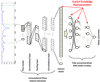 |
Fig. 1 Generic architecture for DL models in Passegger et al. (2020) and the different positions where we concatenated the values of the stellar parameters so that they could be fixed as needed in Run B. |
4 Results
All the results for each star, run, and method are listed in Tables C.1 and C.2. In the following, we discuss the results for each run. As discussed in Sect. 3.1, we compare our results to the literature median, assuming that the literature median represents accurate parameter values for each star, to investigate the consistency of our results over the different runs.
4.1 Run A
In Run A, all teams determined the stellar parameters with their methods without any restrictions. Figure 2 shows the comparison of our results with the literature median for each star. This gives a direct comparison of how each method performed.
4.1.1 Effective temperature
It can be seen in the top panel of Fig. 2 that all the methods are mostly consistent with the literature median (purple dot) within the errors and with only a few outliers. Overall, SteParSyn reproduces the literature values best. Compared to the literature median, the mean difference  is +7 K, meaning that, on average, SteParSyn derived Teff 7 K hotter. Their results fall only two times outside of the error range, which is defined from the combined error bars of the literature median and the respective method for each star. SteParSyn is followed by the Pass19-code, which is on average 50 K hotter than the literature median and falls only once outside the error range. Results from DL lean on the hotter side as well, showing an average of 75 K larger than the literature median, and also falling two times outside the error. In contrast to the previous methods, ODUSSEAS consistently determines Teff cooler than the other methods and, on average, 86 K cooler compared to the literature median. There are only two exceptions when ODUSSEAS derives hotter Teff, namely: J07558+833 and J13005+056. Both stars have large vsini, which is the most likely reason for the larger Teff values. Additionally, ODUSSEAS falls outside the error ranges five times.
Regarding large vsini, the other methods could determine values in good agreement with the literature median for these stars. In preparing Run B, we calculated the median values between the literature and the results of Run A for each star. This overall median (red dot) is also plotted in Fig. 2 for comparison. As can be seen from the plot, the overall median is consistent with the literature median for all stars and sometimes differs only by a few K. Therefore, we considered the overall median as a benchmark value for each star and took it as a fixed value for our Run B.
In order to provide a better visualization of the agreement and spread of our methods, we present modified Bland-Altman plots (Bland & Altman 1986) for each parameter of Run A in the left column of Fig. B.1. These plots show the mean value of two measurements (in our case, e.g., the Teff value from the literature median and one of our methods for each star) on the x-axis, and the difference on the y-axis. To achieve a more uniform distribution of the data points and increase the illustration of potential discrepancies the values can be plotted logarithmically or as ratio instead of the difference, as it is done here. The plot shows the same trends as described above, with DL deriving hotter Teff and ODUSSEAS cooler Teff (see top left panel of Fig. B.1).
Analyzed wavelength regions for Runs C and C2.
4.1.2 Surface gravity
As described in Sect. 2.2.2, ODUSSEAS does not provide log g. From the remaining methods, the Pass19-code performs best. The differences between the results and the literature median are almost always within 0.1 dex, and only once does their value fall outside the error range. On average, log g from the Pass19-code are 0.01 dex higher that the literature median, this difference is nearly negligible. The reason for this is likely the use of evolutionary models to constrain log g. The DL method derives on average 0.06 dex lower log g than the literature median and lies seven times outside of the error. For SteParSyn the log g has values 11 times outside the error range, being, on average, 0.10 dex higher than the literature median. In several cases, log g is significantly higher than the literature median and the other methods. The biggest outlier is GJ 338B, where SteParSyn derives a value of 0.53dex larger than the literature median. A possible explanation for these high values could be either a still remaining degeneracy in the stellar parameter space or the synthetic gap (difference in feature distribution between synthetic and observed spectra). As shown in Marfil et al. (2021), SteParSyn retrieves tentatively higher log g values for the whole CARMENES GTO sample.
In the case of GJ 1002 the overall median for log g represents the median of all our Run A results because there are no literature values for this star. In total, the literature and overall median differ less than 0.1 dex in all cases, except for GJ 493.1, which only has one literature value of 4.5 dex. Therefore, we excluded this star from the analysis of log g in this section.
4.1.3 Metallicity
The bottom panel of Fig. 2 presents the results of all methods for [Fe/H]. Although this parameter is not fixed in Run B, we calculated and plotted an overall median for the purposes of comparison. The Pass19-code performs best compared to the literature median and the other methods. On average, the metallicities are 0.02 dex lower than the literature median. All values agree with each other within their errors, for eight stars the results are within 0.1 dex difference to the literature median, and it is only for five stars that the difference is greater than 0.2 dex. An explanation for this good performance can be the careful line selection of magnetically insensitive lines in the VIS and NIR. The use of multiple lines simultaneously also cancels out most of the effects coming from the synthetic gap, which impacts DL in particular. On this note, DL performs worst when it comes to the metallicity determination. The results for 10 stars, which is more than half of our benchmark sample, lie outside the error range; for 11 stars, the values differ by more than 0.2 dex from the literature median, while only two stars have differences less than 0.1 dex. On average, DL provides metallicities 0.23 dex higher than the literature median, tentatively deriving higher values for all but one star (GJ 205).
ODUSSEAS and SteParSyn determine tentatively lower values for metallicity, with ![Mathematical equation: $\overline{\Delta {\textrm{[Fe/H]}}}$](/articles/aa/full_html/2022/02/aa41920-21/aa41920-21-eq8.png) of –0.14 dex and –0.08 dex, respectively. For ODUSSEAS, two values fall outside the error range, while for SteParSyn it is eight. Eight stars show differences of less than 0.1 dex with ODUSSEAS, and six stars differ by more than 0.2 dex compared to the literature median. For SteParSyn, eight stars fall within 0.1 dex of the literature median and five stars outside of 0.2 dex. All these numbers are summarized in Table 3 for better readability.
of –0.14 dex and –0.08 dex, respectively. For ODUSSEAS, two values fall outside the error range, while for SteParSyn it is eight. Eight stars show differences of less than 0.1 dex with ODUSSEAS, and six stars differ by more than 0.2 dex compared to the literature median. For SteParSyn, eight stars fall within 0.1 dex of the literature median and five stars outside of 0.2 dex. All these numbers are summarized in Table 3 for better readability.
As for Teff and log g, we provide a Bland-Altman plot for [Fe/H] in the bottom left panel of Fig. B.1. In order to avoid a possible division by zero on the y-axis due to values of solar metallicity, we transform [Fe/H] to the logarithmic number ratio of iron and hydrogen atoms via [Fe/H] =  , with
  (see Table 6 in Lodders et al. 2009). Overall, the Pass19-code performs best in log g and [Fe/H] compared to the literature median. For Teff, SteParSyn would be the best choice.
4.2 Run B
For Run B, all teams (except ODUSSEAS, see Sect. 3.2.2) derived only [Fe/H], with Teff and log g fixed to the median values determined from all teams in Run A and literature values. In Fig. 3 we show a comparison between our results and the literature median. Results from Run A are plotted in gray to illustrate the changes between the runs. We can see from this plot that fixing Teff and log g does not improve the metallicities derived with the Pass19-code and DL. For both methods, the discrepancies with regard to the literature median increased. This can be explained by looking at the results for Teff from Run A. If the temperatures were further away from the overall median, which was used to fix this parameter in Run B, then the deviation in metallicity in Run B is larger than in Run A. Some correlation with log g can also be found in some cases. Since in Run B, the parameter determination is reduced to a 1-D problem, there are nolonger any local minima and there is only one best value for metallicity. If the fixed values Teff and log g deviate from the best fitting values found in Run A, the deviation in metallicity will consequently increase as well. Therefore, there will be no improvement regarding metallicity, unless the other parameters Teff and log g can be chosen freely as well. We performed the same analysis of the results here as we did for Run A, with the figures summarized in Table 4. The corresponding Bland–Altman plot is presented on the left in Fig. B.2.
On the other hand, fixing parameters slightly improved the metallicities derived by SteParSyn. The number of stars outside the error range decreased, whereas the number within 0.1 dex increased. A good example here is GJ 338B: from Run A, Teff is close to the literature median, but log g is far off. By fixing log g, the metallicity improves and moves closer to the literature median. This run suggests that there is a dependency on the stellar synthetic spectra used in the analysis. The DL and the Pass19-code both rely on the PHOENIX-ACES model spectra, but do not show any improvements towards literature values, whereas SteParSyn incorporated BT-Settl model atmospheres. Therefore, the next step is for all methods to use the same synthetic models.
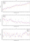 |
Fig. 2 Comparison of Teff (top), log g (middle),and [Fe/H] (bottom) for the different methods in Run A. Each method is indicated with a different symbol and color. The median of all literature values and the median of literature + Run A are shown as purple and red dots, respectively. The x-axis indicates theTeff from the literature median and the top axis shows the Gliese-Jahreiss (GJ) numbers for all sample stars, which are sorted by Teff from the literature median to display any possible trends. |
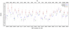 |
Fig. 3 Comparison of [Fe/H] for the different methods in Run B. Each method is indicated with adifferent symbol and color. The gray symbols indicate the results from Run A for comparison. The median of all literature values is shown as purple dots. The x-axis indicates Teff from the median literature, the top axis shows the Gliese–Jahreiss (GJ) numbers for all sample stars. |
Analysis of Run A for Teff (top), log g (middle), and [Fe/H] (bottom).
Analysis of Run B for [Fe/H].
4.3 Runs C and C2
In Run C, all teams incorporated the same normalized PHOENIX-ACES model spectra and derived the parameters from the same wavelength regions. As mentioned in Sect. 3.2.3, we carried out an additional Run C2, using a subset of 35 wavelength regions from Run C, but otherwise identical to Run C. Figure 4 presents a comparison of stellar parameters between Run A and Run C2. A comparison between Run C and C2 is shown in Fig. B.5 and as a Bland-Altman plot in the left column of Fig. B.3 and Fig. B.4. Table 5 summarizes the statistics of Runs C and C2.
Analysis of Run C/C2 for Teff (top), log g (middle), and [Fe/H] (bottom).
4.3.1 Effective temperature
We compared our results from Run C2 to those derived in Run A. Figure 4 shows that the stellar parameters do not improve from Run A to Run C2. This is most evident for Teff, where the 17 stars for SteParSyn, 13 stars for DL, and 12 stars for the Pass19-code show larger deviations to the literature median than in RunA. Analyzing Runs C and C2 shows that stellar parameters derived with DL agree better with the literature median in Run C2 than in Run C. This means an improvement towards Run C2, with all stars being closer to the literature median in Teff compared to Run C. For SteParSyn, the results from Run C and C2 are a bit more ambiguous. Half of the sample stars are closer to the literature median in Run C for Teff, the other half in Run C2. Run C exhibits a larger  of +46 K compared to Run C2 (
 = +0.1 K). Concerning the Pass19-code, Run C is clearly better than Run C2, giving values closer to the literature median. The mean difference,
  , amounts to +60 K, with all values being within the error range for all stars.
4.3.2 Surface gravity
Compared to Run A, the Pass19-code and SteParSyn show similar results as for Teff, with no improvement from Run A to Run C2. On the other hand, 14 stars with log g derived from DL are closer to the literature median in Run C2 than in Run A. For Run C, the results from DL show an improvement towards Run C2 for eleven stars. Only five stars from SteParSyn lie closer to the literature median in Run C2 than in Run C, which clearly favors the results from Run C in this case. For the Pass19-code, the results derived in Run C are tentatively lower than for Run C2. Especially in the case of hotter stars, this means that Run C is closer to the literature median, as can be seen from Fig. B.5.
4.3.3 Metallicity
Similarly to the cases of Teff and log g, the results in metallicity for the Pass19-code and SteParSyn are closer to literature in Run A than in Run C2. However, DL presents a slight improvement, deriving values which are closer to the literature median for 12 stars in metallicity. Using multiple wavelength ranges instead of only one range, as done in Runs A and B, appears to trigger this improvement. Looking at Run C, eight of 18 stars have better values in Run C2 for DL. As for log g, only a small number of five stars shows better results in Run C2 than in Run C for SteParSyn. This could be explained by the fact that SteParSyn is optimized for the wavelength ranges in Run C that are originally used by the method. Analyzing a subset of these ranges, as done in Run C2, does not improve the results. In Run C, the Pass19-code consistently derives too high metallicities, especially for cooler M-dwarfs (see Fig. B.5, bottom panel). The selection of wavelength ranges for Run C2, however, clearly improves the metallicity determination.
Comparing the numbers Table 5 to those of Runs A and B also illustrates the differences and the better performance of Run A. It can be seen, for example, that the number of stars with differences larger than 200 K and 0.2 dex from the literature median significantly increased in Run C2. One exception here is DL, which is able to lower those numbers in Run C2 for [Fe/H].
4.4 Comparison with interferometry
For 11 stars in our study, we can compare our results for Teff and log g to independent measurements coming from interferometry (Boyajian et al. 2012; von Braun et al. 2014; Newton et al. 2015; Rabus et al. 2019). Boyajian et al. (2012) and von Braun et al. (2014) used HIPPARCOS parallaxes (van Leeuwen 2007) to convert the limb-darkened angular stellar diameter, ΘLD, to stellar radius via ΘLD = 2 ⋅ R∕d, whereas Rabus et al. (2019) used Gaia DR2 data (Gaia Collaboration 2018). Newton et al. (2015) collected interferometric radii from the literature. When there was more than one measurement per star, they calculated the weighted mean. Then, Teff can be derived from the Stefan-Boltzmann law,  (with T0 = 2341 K), when the bolometric flux Fbol is known. Boyajian et al. (2012) and von Braun et al. (2014) produced spectral energy distributions (SEDs) using flux-calibrated photometry from the literature. Rabus et al. (2019) estimated Fbol by integrating the flux from synthetic photometric flux points using PHOENIX-ACES synthetic spectra. Newton et al. (2015) presented interferometric Teff from Mann et al. (2013b) and updated Teff for three stars following their approach. Mann et al. (2013b) determined Fbol by comparing the measured fluxes from observed visual and NIR spectra, incorporating BT-Settl synthetic models to cover wavelength gaps in the spectra, to photometric fluxes using a correction factor to adjust the overall flux level. From the stellar radius and mass, log g can be calculated via g = GM∕R2. This requires the stellar mass, which cannot be measured from interferometry. Therefore, Boyajian et al. (2012) and Rabus et al. (2019) used the K-band mass-luminosity relation from Henry & McCarthy (1993), and from Benedict et al. (2016) and Mann et al. (2019), respectively. von Braun et al. (2014) determined stellar mass by deriving a mass-radius relation from the results from Boyajian et al. (2012). Although Teff can be derived independently from interferometry, log g can be seen as semi-independent, since it involves interferometric radii, but also empirical mass-radius or mass-luminosity relations. Therefore, such quasi-interferometric log g tend to possess a tentatively higher level of accuracy than log g derived from, for instance, synthetic model fits alone; thus, the former can be used as a reliable comparison. A comparison plot is shown in Fig. 5. We calculated the mean difference, standard deviation, and Pearson correlation coefficient (rP) between our results and the literature, presented in Table 6. A good consistency between the samples would result in a low mean difference and standard deviation, as well as a Pearson correlation coefficient close to 1.
For Run A, SteParSyn agrees quite well with interferometry in Teff with  K, followed by the Pass19-code, which gives slightly hotter values with
  K compared to interferometry. Also, DL is on the hotter side (
 K), whereas ODUSSEAS, as mentioned before, derived tentatively cooler temperatures (
 K). In Run C (which corresponds to Run C* for ODUSSEAS), temperatures from DL and ODUSSEAS are shifted more towards the hotter side, bringing ODUSSEAS closer to the interferometric values (
 K). This is the same behavior seen in Fig. 6. In contrast, the Pass19-code provides cooler temperatures, but still mostly consistent with those from interferometry (
 K). SteParSyn performs similar to Run A, however with some larger spread at low and high temperatures, which is represented in a higher standard deviation compared to Run A. This is similar for Run C2, where SteParSyn again yields some cooler temperatures compared to Run C. Overall, SteParSyn does best in Run A, where it shows the lowest standard deviation and highest rP, similarly to the Pass19-code. On the other hand, DL shows a better 1:1 relation in Run C2, represented by the larger rP (see Table 6). This indicates that the selected wavelength ranges in Run C2 lead to an improvement in the results, although there seems to be a general offset towards hotter temperatures compared to interferometry. Again, this is also illustrated in Fig. 6.
For log g, the Pass19-code is closest to the quasi-interferometric log g for all runs, which is most likely due to the use of evolutionary models in the method. However, the values are slightly lower than those in the literature, on average. The smallest standard deviation and highest rP is presented by Run A, as for Teff. The results given by the Pass19-code in Run C are systematically lower than interferometric ones, but they improve in Run C2. In general, DL follows the relation, but those results are lower as well. A great improvement is shown for DL in Run C and even more in Run C2, where  decreases toas low as +0.001 dex, which can be clearly attributed to the use of multiple wavelength ranges. Overall, the values from SteParSyn show a large spread with a high standard deviation and low rP. The spread is persistent in Runs C and C2, although the mean difference of all SteParSyn values moves closer to the 1:1 relation.
Overall, this comparison is very similar to the comparison of the literature median and yet another indication that, for most stars, Run A gives very good results compared to the literature median, with the exception of DL, where the analysis of multiple wavelength ranges results in better measurements of log g and a higher correlation in Teff. A similar analysis could be done for metallicity, should there be independent measurements from a hotter FGK-type binary companion available.
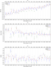 |
Fig. 4 Comparison of Teff (top), log g (middle), and [Fe/H] (bottom) for the different methods in Run C2. Each method is indicated with a different symbol and color. The gray symbols indicate the results from Run A for comparison. The median of all literature values is shown as purple dots. The x-axis indicates Teff from the literature median, the top axis shows the Gliese–Jahreiss (GJ) numbers for all sample stars. |
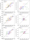 |
Fig. 5 Comparison of our results for Teff (left column) and log g (right column) from Run A (top), Run C (middle), and Run C2 (bottom) with interferometric radii from Boyajian et al. (2012), von Braun et al. (2014), Newton et al. (2015), and Rabus et al. (2019). If more than one value exists for a star in literature, we plot the mean with the RMSE for better readability. Results from ODUSSEAS in Run C correspond to their Run C*. The black line indicates the 1:1 relationship. |
Mean difference between our results and interferometric literature values,  /
/  , standard deviation of the mean difference, std. dev., and Pearson correlation coefficients, rP, for Teff / log g.
5 Discussion
We compare the results from all runs for each method in order to analyze which run gives the best results, namely, which run offers the most stars with values that are closest to the literature median. For example, in case of the Pass19-code, each star has four determined [Fe/H] values, derived in Runs A, B, C, and C2. For each value, we calculated the difference from the literature median to find the minimum difference, for example, for Run A. This particular star then counts toward Run A. The procedure is repeated for all stars and for all three stellar parameters. As a consequence, the sum over all runs for each stellar parameter is always 18, except for log g, where we excluded GJ 1002 from the analysis. In this way, we can assess which run performed best for each stellar parameter.
Figure 6 shows this number of stars for all parameters and methods. From this, we can see that for Teff, all methods but ODUSSEAS perform best in Run A. Generally, the Pass19-code works better in Run A than in the other Runs. Runs C and C2 show a similar performance for [Fe/H].
The DL results get closer to the literature median for [Fe/H] and log g in Runs C and C2, respectively. Since the continuum normalization and synthetic spectra are the same as the ones used in Runs A and B, the only explanation for the improvement is the different wavelength regions. Then, DL can determine [Fe/H] and log g significantly better by taking into account more wavelength regions than just the one between 8800 Å and 8835 Å, although this region seems to work well for Teff alone.
Similar to the Pass19-code, SteParSyn generally shows the best performance in Run A, with good results declining towards Runs C andC2. An exception is metallicity, which is best in Run B, directly followed by Run A. This indicates that the metallicity determinations with SteParSyn could be improved by taking independent estimates and fixing Teff and log g. The stellar parameters derived in Runs C and C2 show tentatively larger deviations from the literature median than Run A, which is probably due to the different synthetic spectra used. This implies that SteParSyn is optimized for the analysis of their selected wavelength ranges with BT-Settl models.
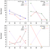 |
Fig. 6 Number of stars for each run where the stellar parameter lies closest to the literature median. Each method is shown in a separate panel. We note that ODUSSEAS does not provide log g, and their Run C* differs from our Runs C and C2 due to restrictions in the method itself. |
5.1 ODUSSEAS Run C*
As described in Sect. 3.2.3, ODUSSEAS was only able to use the bluest wavelength ranges provided for Runs C and C2. Therefore, the results cannot be directly compared to the other methods. However, it is possible to assess the performance of the algorithm itself. Since ODUSSEAS does not rely on synthetic model spectra, and a different continuum normalization does not affect the measurement of pEWs, the only difference between Runs A and C* is the choice of the wavelength ranges. In the bottom right panel of Fig. 6, it can be seen that ODUSSEAS derives the best metallicities for all 18 stars in Run A. For Teff, Run A shows tentatively lower values compared to other methods and the literature. However, their modified Run C* gives significantly better results. From this, we can conclude that the wavelength ranges used in Run A are very good for deriving metallicity, but seem to be less sensitive to Teff. On the other hand, the ranges used in Run C* appear to be more appropriate when it comes to temperature determination.
5.2 Consistency between methods
As a last step, we analyzed the consistency between the methods we employed in this experiment. A statistical analysis similar to Table 6 is presented in Table 7. We compare each method to each of the other methods to reveal trends. We plotted all these combination for further visualization in Figs. B.6–B.8 for Teff, log g, and [Fe/H] for Run A; [Fe/H] for Run B is presented in Fig. B.9, Teff, log g, and [Fe/H] for Run C in Figs. B.10–B.12, and Teff, log g, and [Fe/H] for Run C2 in Figs. B.13–B.15. The corresponding Bland-Altman plots similar to the literature comparison are shown in the right columns of Figs. B.1–B.4.
5.2.1 Run A
For Teff, SteParSyn and the Pass19-code show the best correlation with rP of 0.974, also being the only methods with a spread, namely, a standard deviation of less than 100 K between them. Both methods compare well with DL, although DL shows higher deviations at higher Teff. As illustrated in previous comparisons (see Figs. 2 and 5), ODUSSEAS derives much lower Teff values, on average, 130 K cooler compared to the other methods. Pass19-code and DL correlate quite well in log g, whereas SteParSyn exhibits a large spread compared to both other methods (see also Figs. 2 and 5).
SteParSyn, the Pass19-code, and ODUSSEAS are in good agreement in [Fe/H], having small mean differences and a large rP. The direct comparison between SteParSyn and ODUSSEAS displays a slightly larger spread and, therefore, a smaller rP. For DL, it derives much higher [Fe/H] values, which are, on average, 0.3 dex more metal-rich compared to the other methods. This behaviour can also be seen in Fig. 2.
5.2.2 Run B
As in Run A, SteParSyn and the Pass19-code are most consistent with a small mean difference of only 0.03 dex, and a similar standard deviation. However, the values are not so well correlated, exhibiting a slightly smaller rP of 0.784 (compared to rP = 0.804 in Run A). Here, DL performs even worse than it does in Run A, with ![Mathematical equation: $\overline{\Delta {\textrm{[Fe/H]}}}$](/articles/aa/full_html/2022/02/aa41920-21/aa41920-21-eq22.png) being –0.33 dex and –0.36 dex compared to the Pass19-code and SteParSyn, respectively.
being –0.33 dex and –0.36 dex compared to the Pass19-code and SteParSyn, respectively.
5.2.3 Runs C and C2
As described in Sects. 3.2.3 and 4.4, ODUSSEAS was only able to use wavelength ranges between 5300 and 6900 Å. Therefore, a direct comparison of results from this Run C* with the results from Runs C and C2 from the other methods is not meaningful. However, we included ODUSSEAS in our analysis here for completeness and to visualize relative changes between Runs C and C2 for the other methods.
A comparison of Run C with C2 reveals only minor differences for Teff. It can be seen from the numbers in Table 7 and the plot in Fig. B.10 that DL performs a bit better in Run C2, where it derives slightly lower Teff and therefore exhibits a smaller  compared to the other methods. SteParSyn and the Pass19-code show a somewhat smaller
  and spread in Run C. This is also clearly shown by the comparison of the Pass19-code and ODUSSEAS in Runs C and C2. Since for both runs the Pass19-code is compared to Run C* of ODUSSEAS, relative improvements between the runs are revealed. Overall, it can be said that the correlation coefficients for Teff are slightly greater in Run C compared to Run C2.
On the other hand, there is almost no correlation in log g for any of the methods. The only notable improvement toward Run C2 is given between the Pass19-code and DL, which present a little higher correlation and smaller  in Run C2. This can be attributed to an improvement of DL in Run C2, as already described in Sects. 4 and 4.4.
A clear difference can be seen for [Fe/H] between Runs C and C2 (see Figs. B.12 and B.15). In Run C, all methods appear more separated, also having higher mean differences. They determine, in general, higher [Fe/H] values, especially the Pass19-code, which is depicted in Fig. B.5 as well. For Run C2, the derived values are more metal-poor, which causes the results to move closer together for all methods. This reduces the mean differences, although the spread and correlation coefficient are not necessarily improved for all methods.
Overall, the closest correlation between the methods for all stellar parameters is found in Run A, however we can see some trends. The determination of log g with SteParSyn is generally not very well constrained: it has a large mean difference and spread compared to the other methods. The correlation increases toward Run C and C2, however the reason for this is not clear. In particular, ODUSSEAS shows the best consistency in Teff in Run C*, when compared to Run C using the other methods, with the smallest mean difference and a slightly better rP than in Run A. For [Fe/H], Run A as well as Run C2 show small ![Mathematical equation: $\overline{\Delta{\textrm{[Fe/H]}}}$](/articles/aa/full_html/2022/02/aa41920-21/aa41920-21-eq26.png) in general; however, in Run C2 the spread is larger and rP is smaller, therefore, the consistency in [Fe/H] is better in Run A. Only DL is able to improve the consistency toward Runs C and C2, with negligible differences between C and C2. Consequently, rP increases and
in general; however, in Run C2 the spread is larger and rP is smaller, therefore, the consistency in [Fe/H] is better in Run A. Only DL is able to improve the consistency toward Runs C and C2, with negligible differences between C and C2. Consequently, rP increases and ![Mathematical equation: $\overline{\Delta{\textrm{[Fe/H]}}}$](/articles/aa/full_html/2022/02/aa41920-21/aa41920-21-eq27.png) decreases.
decreases.
Possible improvements to increase the consistency are very specific to the method and there is no general recipe. For DL, the values in [Fe/H] are tentatively too high, using more wavelength ranges can improve [Fe/H] in Runs C and C2. However, for the determination of Teff, one wavelength range serves well. We see that ODUSSEAS derives consistently lower Teff, and the use of different wavelength ranges, as done in Run C*, would increase the level of consistency with our other methods. The analysis in this section confirms our findings in Sects. 4 and 4.4.
Statistical analysis between our methods for Runs A, B, C, and C2.
6 Summary and conclusions
In this study, we applied four different methods, including synthetic spectral fitting, pEW measurements, and machine learning, to derive the stellar parameters Teff, log g, and [Fe/H] for a sample of 18 M dwarfs from high-resolution and high-S/N CARMENES spectra. Our analysis consisted of four different runs: Run A allowed each team to use their method without restrictions, Run B fixed Teff and log g to derive only [Fe/H], and for Runs C and C2, all the teams incorporated the same synthetic model spectra, continuum normalization method, and wavelength ranges.
Although we provided several new stellar parameters for our sample, it was not our goal to measure more precise or accurate parameters for these stars in the context of a catalog, but to identify and understand discrepancies in the parameters between our groups, namely, the different parameter determination methods, with the aim to minimize these discrepancies in order to make a step forward to more consistent parameter determinations. At the beginning of this experiment, we expected that a standardization of underlying synthetic models and wavelength ranges, along with a reduction of the dimension of the parameter space by fixing stellar parameters would account for the inconsistencies between our results and literature medians. Therefore, we assumed to find the best agreement between our methods and with comparisons to the literature in Runs C and C2. However, we found that this is not necessarily the case as it is for FGK stars (e.g., Jofré et al. 2014, 2017), and that our methods generally show the greatest consistency with the literature values when used in their original setting without any standardization. In general, the mean differences to the literature median are below 100 K in Teff for all methods,and also below 0.1 dex in [Fe/H] for the Pass19-code and SteParSyn. In Runs C and C2, these differences increase significantly,up to over 200 K and 0.3 dex for some of our methods.
This consistency in Run A is an indication that each team successfully calibrated their methods and optimized them to the use of certain wavelength ranges and synthetic spectra. It also implies that there might be other components responsible for the remaining differences that we see in the stellar parameters, which requires a more thorough and in-depth investigation of the methods themselves and the underlying concepts. One example is stellar atmosphere models and their corresponding spectra, where, despite constant improvements, they still suffer from some deficiencies. Various sets of synthetic spectra also show discrepancies when comparing the same spectral lines, due to the use of different equations of state, line lists, and other hyper-parameters. It cannot be excluded that these deviations contribute to the disagreements in derived stellar parameters found in this work. However, we were able to shed some light on deficiencies of some methods, for instance, showing that the DL method would benefit from the use of multiple wavelength ranges and that ODUSSEAS could improve the Teff determination by using different sets of lines or, most importantly, by using a new reference Teff scale based on interferometry (Khata et al. 2021). This possibility is currently being explored and is expected to be implemented as an optionin an upgraded version of the tool.
Acknowledgements
We thank an anonymous referee for helpful comments that improved the quality of this paper. CARMENES is an instrument for the Centro Astronómico Hispano-Alemán de Calar Alto (CAHA, Almería, Spain). CARMENES is funded by the German Max-Planck-Gesellschaft (MPG), the Spanish Consejo Superior de Investigaciones Científicas (CSIC), European Regional Development Fund (ERDF) through projects FICTS-2011-02, ICTS-2017-07-CAHA-4, and CAHA16-CE-3978, and the members of the CARMENES Consortium (Max-Planck-Institut für Astronomie,Instituto de Astrofísica de Andalucía, Landessternwarte Königstuhl, Institut de Ciències de l’Espai, Insitut für Astrophysik Göttingen, Universidad Complutense de Madrid, Thüringer Landessternwarte Tautenburg,Instituto de Astrofísica de Canarias, Hamburger Sternwarte, Centro de Astrobiología and Centro Astronómico Hispano-Alemán), with additional contributions by the Spanish Ministry of Economy, the German Science Foundation through the Major Research Instrumentation Programme and DFG Research Unit FOR2544 “Blue Planets around Red Stars”, the Klaus Tschira Stiftung, the states of Baden-Württemberg and Niedersachsen, and by the Junta de Andalucía. E.D.M. and A.A.K. acknowledge the support by the Investigador FCT contract IF/00849/2015/CP1273/CT0003. We acknowledge financial support from NASA through grant NNX17AG24G, the Agencia Estatal de Investigación of the Ministerio de Ciencia through fellowship FPU15/01476, Innovación y Universidades and the ERDF through projects PID2019-109522GB-C51/2/3/4, AYA2016-79425-C3-1/2/3-P and AYA2018-84089, the Fundação para a Ciência e a Tecnologia through and ERDF through grants UID/FIS/04434/2019, UIDB/04434/2020 and UIDP/04434/2020, PTDC/FIS-AST/28953/2017, and PTDC/FIS-AST/32113/2017, and COMPETE2020 - Programa Operacional Competitividade e Internacionalização POCI-01-0145-FEDER-028953, and POCI-01-0145-FEDER-032113. This research has been funded by the Spanish State Research Agency (AEI) Project No. MDM-2017-0737 Unidad de Excelencia “María de Maeztu" – Centro de Astrobiología (CSIC/INTA).
Appendix A Literature summary of sample stars
Collection of stellar parameters from the literature for the selected sample of benchmark stars.
Appendix B Additional plots
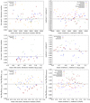 |
Fig. B.1 Modified Bland-Altman plot for Run A, showing the mean of two methods on the x-axis and the ratioon the y-axis. The left column presents the comparison between the literature median and our methods (color-coded) for Teff (top), log g (middle), and [Fe/H] (bottom). The right column presents the comparison between our methods. Each symbol represents a different combination of our methods, as shown in the legend. For [Fe/H] the y-axis shows the ratio of the number of Fe and H atoms in order to avoid division by zero. See text for details. |
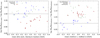 |
Fig. B.2 Modified Bland-Altman plot for [Fe/H] in Run B, showing the mean of two methods on the x-axis and on the y-axis the ratio of the number of Fe and H atoms in order to avoid division by zero. The left plot presents the comparison between the literature median and our methods (color-coded). The right plot presents the comparison between our methods. Each symbol represents a different combinationof our methods, as shown in the legend. |
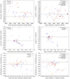 |
Fig. B.3 Modified Bland-Altman plot for Run C, showing the mean of two methods on the x-axis and the ratioon the y-axis. The left column presents the comparison between the literature median and our methods (color-coded) for Teff (top), log g (middle), and [Fe/H] (bottom). The right column presents the comparison between our methods. Each symbol represents a different combination of our methods, as shown in the legend. For [Fe/H] the y-axis shows the ratio of the number of Fe and H atoms in order to avoid division by zero. See text for details. |
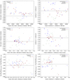 |
Fig. B.4 Modified Bland-Altman plot for Run C2, showing the mean of two methods on the x-axis and the ratioon the y-axis. The left column presents the comparison between the literature median and our methods (color-coded) for Teff (top), log g (middle), and [Fe/H] (bottom). The right column presents the comparison between our methods. Each symbol represents a different combination of our methods, as shown in the legend. For [Fe/H] the y-axis shows the ratio of the number of Fe and H atoms in order to avoid division by zero. See text for details. |
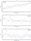 |
Fig. B.5 Comparison of Teff (top), log g (middle), and [Fe/H] (bottom) for the different methods in Run C2. Each method is indicated with a different symbol and color. The gray symbols indicate the results from Run C for comparison. The median of all literature values is shown as purple dots. The x-axis indicates Teff from the literature median, the top axis shows the Gliese-Jahreiss (GJ) numbers for all sample stars. |
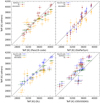 |
Fig. B.6 Comparison between our methods, showing the derived Teff in Run A. Each method is indicated by a different color and symbol. Each panel compares one method (denoted by the x-axis label) to all other methods. |
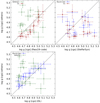 |
Fig. B.7 Comparison between our methods, showing the derived log g in Run A. Each method is indicated by a different color and symbol. Each panel compares one method (denoted by the x-axis label) to all other methods. ODUSSEAS did not derive log g. |
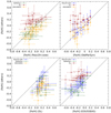 |
Fig. B.8 Comparison between our methods, showing the derived [Fe/H] in Run A. Each method is indicated by a different color and symbol. Each panel compares one method (denoted by the x-axis label) to all other methods. |
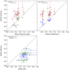 |
Fig. B.9 Comparison between our methods, showing the derived [Fe/H] in Run B. Each method is indicated by a different color and symbol. Each panel compares one method (denoted by the x-axis label) to allother methods. ODUSSEAS did not participate in Run B. |
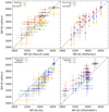 |
Fig. B.10 Comparison between our methods, showing the derived Teff in Run C. Each method is indicated by a different color and symbol. Each panel compares one method (denoted by the x-axis label) to all other methods. The values from ODUSSEAS correspond to Run C*. |
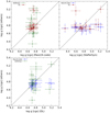 |
Fig. B.11 Comparison between our methods, showing the derived log g in Run C. Each method is indicated by a different color and symbol. Each panel compares one method (denoted by the x-axis label) to all other methods. ODUSSEAS did not derive log g. |
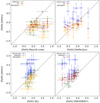 |
Fig. B.12 Comparison between our methods, showing the derived [Fe/H] in Run C. Each method is indicated by a different color and symbol. Each panel compares one method (denoted by the x-axis label) to all other methods. The values from ODUSSEAS correspond to Run C*. |
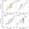 |
Fig. B.13 Comparison between our methods, showing the derived Teff in RunC2. Each method is indicated by a different color and symbol. Each panel compares one method (denoted by the x-axis label) to all other methods. The values from ODUSSEAS correspond to Run C*. |
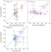 |
Fig. B.14 Comparison between our methods, showing the derived log g in RunC2. Each method is indicated by a different color and symbol. Each panel compares one method (denoted by the x-axis label) to all other methods. ODUSSEAS did not derive log g. |
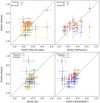 |
Fig. B.15 Comparison between our methods, showing the derived [Fe/H] in Run C2. Each method is indicated by a different color and symbol. Each panel compares one method (denoted by the x-axis label) to all other methods. The values from ODUSSEAS correspond to Run C*. |
Appendix C Results
Tables C.1 and C.2 are available in their entirety in a machine- readable form at the CDS. An excerpt is shown here for guidanceregarding their form and content.
Stellar parameters for each method from Runs A and B.
Stellar parameters for each method from Runs C and C2.
References
- Allard, F., Hauschildt, P. H., Alexander, D. R., Tamanai, A., & Schweitzer, A. 2001, ApJ, 556, 357 [Google Scholar]
- Allard, F., Homeier, D., & Freytag, B. 2011, in 16th Cambridge Workshop on Cool Stars, Stellar Systems, and the Sun, eds. C. Johns-Krull, M. K. Browning, & A. A. West, ASP Conf. Ser., 448, 91 [Google Scholar]
- Allard, F., Homeier, D., & Freytag, B. 2012, Philos. Trans. R. Soc. Lond. A, 370, 2765 [Google Scholar]
- Allard, F., Homeier, D., Freytag, B., et al. 2013, Mem. Soc. Astron. Ital. Suppl., 24, 128 [Google Scholar]
- Alonso-Floriano, F. J., Morales, J. C., Caballero, J. A., et al. 2015, A&A, 577, A128 [NASA ADS] [CrossRef] [EDP Sciences] [Google Scholar]
- Antoniadis-Karnavas, A., Sousa, S. G., Delgado-Mena, E., et al. 2020, A&A, 636, A9 [NASA ADS] [CrossRef] [EDP Sciences] [Google Scholar]
- Asplund, M., Grevesse, N., Sauval, A. J., & Scott, P. 2009, ARA&A, 47, 481 [NASA ADS] [CrossRef] [Google Scholar]
- Bayo, A., Rodrigo, C., Barrado Y Navascués, D., et al. 2008, A&A, 492, 277 [NASA ADS] [CrossRef] [EDP Sciences] [Google Scholar]
- Benedict, G. F., Henry, T. J., Franz, O. G., et al. 2016, AJ, 152, 141 [Google Scholar]
- Berger, D. H., Gies, D. R., McAlister, H. A., et al. 2006, ApJ, 644, 475 [NASA ADS] [CrossRef] [Google Scholar]
- Birky, J., Hogg, D. W., Mann, A. W., & Burgasser, A. 2020, ApJ, 892, 31 [Google Scholar]
- Bland, J. M., & Altman, D. G. 1986, The Lancet, 327, 307 [Google Scholar]
- Borsa, F., Allart, R., Casasayas-Barris, N., et al. 2021, A&A, 645, A24 [EDP Sciences] [Google Scholar]
- Boyajian, T. S., von Braun, K., van Belle, G., et al. 2012, ApJ, 757, 112 [Google Scholar]
- Bressan, A., Marigo, P., Girardi, L., et al. 2012, MNRAS, 427, 127 [NASA ADS] [CrossRef] [Google Scholar]
- Burn, R., Schlecker, M., Mordasini, C., et al. 2021, A&A, 656, A72 [NASA ADS] [CrossRef] [EDP Sciences] [Google Scholar]
- Caballero, J. A., Cortés-Contreras, M., Alonso-Floriano, F. J., et al. 2016a, in 19th Cambridge Workshop on Cool Stars, Stellar Systems, and the Sun (CS19), 148 [Google Scholar]
- Caballero, J. A., Guàrdia, J., López del Fresno, M., et al. 2016b, in Proc. SPIE, 9910, Observatory Operations: Strategies, Processes, and Systems VI, 99100E [Google Scholar]
- Casagrande, L., Flynn, C., & Bessell, M. 2008, MNRAS, 389, 585 [Google Scholar]
- Chen, Y., Girardi, L., Bressan, A., et al. 2014, MNRAS, 444, 2525 [Google Scholar]
- Chen, Y., Bressan, A., Girardi, L., et al. 2015, MNRAS, 452, 1068 [Google Scholar]
- Cifuentes, C., Caballero, J. A., Cortés-Contreras, M., et al. 2020, A&A, 642, A115 [NASA ADS] [CrossRef] [EDP Sciences] [Google Scholar]
- Claret, A., Hauschildt, P. H., & Witte, S. 2012, A&A, 546, A14 [NASA ADS] [CrossRef] [EDP Sciences] [Google Scholar]
- Dittmann, J. A., Irwin, J. M., Charbonneau, D., & Newton, E. R. 2016, ApJ, 818, 153 [NASA ADS] [CrossRef] [Google Scholar]
- Dotter, A., Chaboyer, B., Jevremović, D., et al. 2008, ApJS, 178, 89 [Google Scholar]
- Fabbro, S., Venn, K. A., O’Briain, T., et al. 2018, MNRAS, 475, 2978 [Google Scholar]
- Figueira, P., Adibekyan, V. Z., Oshagh, M., et al. 2016, A&A, 586, A101 [NASA ADS] [CrossRef] [EDP Sciences] [Google Scholar]
- Gaia Collaboration (Brown, A. G. A., et al.) 2018, A&A, 616, A1 [NASA ADS] [CrossRef] [EDP Sciences] [Google Scholar]
- Gaidos, E., & Mann, A. W. 2014, ApJ, 791, 54 [Google Scholar]
- Gaidos, E., Mann, A. W., Lépine, S., et al. 2014, MNRAS, 443, 2561 [Google Scholar]
- Gustafsson, B., Edvardsson, B., Eriksson, K., et al. 2008, A&A, 486, 951 [NASA ADS] [CrossRef] [EDP Sciences] [Google Scholar]
- Hauschildt, P. H. 1992, J. Quant. Spec. Radiat. Transf., 47, 433 [NASA ADS] [CrossRef] [Google Scholar]
- Hauschildt, P. H. 1993, J. Quant. Spec. Radiat. Transf., 50, 301 [NASA ADS] [CrossRef] [Google Scholar]
- Hauschildt, P. H., & Baron, E. 1999, J. Comput. Appl. Math., 109, 41 [NASA ADS] [CrossRef] [Google Scholar]
- Hauschildt, P. H., Baron, E., & Allard, F. 1997, ApJ, 483, 390 [Google Scholar]
- Hauschildt, P. H., Allard, F., & Baron, E. 1999, ApJ, 512, 377 [Google Scholar]
- Heiter, U., Lind, K., Bergemann, M., et al. 2021, A&A, 645, A106 [EDP Sciences] [Google Scholar]
- Henry, T. J., & McCarthy, Donald W., J. 1993, AJ, 106, 773 [NASA ADS] [CrossRef] [Google Scholar]
- Henry, T. J., Jao, W.-C., Winters, J. G., et al. 2016, in Am. Astron. Soc. Meet. Abstr., 227, 142.01 [NASA ADS] [Google Scholar]
- Hinkel, N. R., Young, P. A., Pagano, M. D., et al. 2016, ApJS, 226, 4 [CrossRef] [Google Scholar]
- Houdebine, É. R., Mullan, D. J., Doyle, J. G., et al. 2019, AJ, 158, 56 [NASA ADS] [CrossRef] [Google Scholar]
- Husser, T.-O., Wende-von Berg, S., Dreizler, S., et al. 2013, A&A, 553, A6 [NASA ADS] [CrossRef] [EDP Sciences] [Google Scholar]
- Jofré, P., Heiter, U., Soubiran, C., et al. 2014, A&A, 564, A133 [NASA ADS] [CrossRef] [EDP Sciences] [Google Scholar]
- Jofré, P., Heiter, U., Soubiran, C., et al. 2015, A&A, 582, A81 [Google Scholar]
- Jofré, P., Heiter, U., Worley, C. C., et al. 2017, A&A, 601, A38 [Google Scholar]
- Johnson, S. G., & Wuttke, J. 2019, libcerf, numeric library for complex error functions, version 1.13, https://jugit.fz-juelich.de/mlzu/libcerf [Google Scholar]
- Kausch, W., Noll, S., Smette, A., et al. 2014, in Astronomical Data Analysis Software and Systems XXIII, eds. N. Manset, & P. Forshay, ASP Conf. Ser., 485, 403 [NASA ADS] [Google Scholar]
- Khata, D., Mondal, S., Das, R., Ghosh, S., & Ghosh, S. 2020, MNRAS, 493, 4533 [NASA ADS] [CrossRef] [Google Scholar]
- Khata, D., Mondal, S., Das, R., & Baug, T. 2021, MNRAS, 507, 1869 [NASA ADS] [CrossRef] [Google Scholar]
- Lépine, S., Hilton, E. J., Mann, A. W., et al. 2013, AJ, 145, 102 [Google Scholar]
- Lindgren, S., Heiter, U., & Seifahrt, A. 2016, A&A, 586, A100 [NASA ADS] [CrossRef] [EDP Sciences] [Google Scholar]
- Lodders, K., Palme, H., & Gail, H. P. 2009, Landolt Börnstein, 4B, 712 [Google Scholar]
- Majewski, S. R., Schiavon, R. P., Frinchaboy, P. M., et al. 2017, AJ, 154, 94 [NASA ADS] [CrossRef] [Google Scholar]
- Maldonado, J., Affer, L., Micela, G., et al. 2015, A&A, 577, A132 [NASA ADS] [CrossRef] [EDP Sciences] [Google Scholar]
- Mann, A. W., Brewer, J. M., Gaidos, E., Lépine, S., & Hilton, E. J. 2013a, AJ, 145, 52 [Google Scholar]
- Mann, A. W., Gaidos, E., & Ansdell, M. 2013b, ApJ, 779, 188 [NASA ADS] [CrossRef] [Google Scholar]
- Mann, A. W., Deacon, N. R., Gaidos, E., et al. 2014, AJ, 147, 160 [CrossRef] [Google Scholar]
- Mann, A. W., Feiden, G. A., Gaidos, E., Boyajian, T., & von Braun, K. 2015, ApJ, 804, 64 [Google Scholar]
- Mann, A. W., Dupuy, T., Kraus, A. L., et al. 2019, ApJ, 871, 63 [Google Scholar]
- Marfil, E., Tabernero, H. M., Montes, D., et al. 2020, MNRAS, 492, 5470 [NASA ADS] [CrossRef] [Google Scholar]
- Marfil, E., Tabernero, H. M., Montes, D., et al. 2021, A&A, 656, A162 [NASA ADS] [CrossRef] [EDP Sciences] [Google Scholar]
- Nagel, E., Czesla, S., Kaminski, A., et al. 2021, A&A, submitted [Google Scholar]
- Nemravová, J. A., Harmanec, P., Brož, M., et al. 2016, A&A, 594, A55 [Google Scholar]
- Neves, V., Bonfils, X., Santos, N. C., et al. 2012, A&A, 538, A25 [NASA ADS] [CrossRef] [EDP Sciences] [Google Scholar]
- Neves, V., Bonfils, X., Santos, N. C., et al. 2013, A&A, 551, A36 [NASA ADS] [CrossRef] [EDP Sciences] [Google Scholar]
- Neves, V., Bonfils, X., Santos, N. C., et al. 2014, A&A, 568, A121 [NASA ADS] [CrossRef] [EDP Sciences] [Google Scholar]
- Newton, E. R., Charbonneau, D., Irwin, J., et al. 2014, AJ, 147, 20 [Google Scholar]
- Newton, E. R., Charbonneau, D., Irwin, J., & Mann, A. W. 2015, ApJ, 800, 85 [NASA ADS] [CrossRef] [Google Scholar]
- Önehag, A., Heiter, U., Gustafsson, B., et al. 2012, A&A, 542, A33 [NASA ADS] [CrossRef] [EDP Sciences] [Google Scholar]
- Parzen, E. 1962, Ann. Math. Stat., 33, 1065 [Google Scholar]
- Passegger, V. M., Wende-von Berg, S., & Reiners, A. 2016, A&A, 587, A19 [NASA ADS] [CrossRef] [EDP Sciences] [Google Scholar]
- Passegger, V. M., Reiners, A., Jeffers, S. V., et al. 2018, A&A, 615, A6 [NASA ADS] [CrossRef] [EDP Sciences] [Google Scholar]
- Passegger, V. M., Schweitzer, A., Shulyak, D., et al. 2019, A&A, 627, A161 [NASA ADS] [CrossRef] [EDP Sciences] [Google Scholar]
- Passegger, V. M., Bello-García, A., Ordieres-Meré, J., et al. 2020, A&A, 642, A22 [NASA ADS] [CrossRef] [EDP Sciences] [Google Scholar]
- Plez, B. 2012, Turbospectrum: Code for spectral synthesis [Google Scholar]
- Quirrenbach, A., Amado, P. J., Ribas, I., et al. 2018, SPIE Conf. Ser., 10702, 107020W [Google Scholar]
- Rabus, M., Lachaume, R., Jordán, A., et al. 2019, MNRAS, 484, 2674 [Google Scholar]
- Reiners, A., Zechmeister, M., Caballero, J. A., et al. 2018, A&A, 612, A49 [NASA ADS] [CrossRef] [EDP Sciences] [Google Scholar]
- Reylé, C., Jardine, K., Fouqué, P., et al. 2021, A&A, 650, A201 [Google Scholar]
- Rojas-Ayala, B., Covey, K. R., Muirhead, P. S., & Lloyd, J. P. 2012, ApJ, 748, 93 [Google Scholar]
- Rosenblatt, M. 1956, Ann. Math. Stat., 27, 832 [Google Scholar]
- Sarmento, P., Rojas-Ayala, B., Delgado Mena, E., & Blanco-Cuaresma, S. 2021, A&A, 649, A147 [NASA ADS] [CrossRef] [EDP Sciences] [Google Scholar]
- Schöfer, P., Jeffers, S. V., Reiners, A., et al. 2019, A&A, 623, A44 [Google Scholar]
- Schweitzer, A., Passegger, V. M., Cifuentes, C., et al. 2019, A&A, 625, A68 [NASA ADS] [CrossRef] [EDP Sciences] [Google Scholar]
- Ségransan, D., Kervella, P., Forveille, T., & Queloz, D. 2003, A&A, 397, L5 [NASA ADS] [CrossRef] [EDP Sciences] [Google Scholar]
- Slumstrup, D., Grundahl, F., Silva Aguirre, V., & Brogaard, K. 2019, A&A, 622, A111 [NASA ADS] [CrossRef] [EDP Sciences] [Google Scholar]
- Smette, A., Sana, H., Noll, S., et al. 2015, A&A, 576, A77 [NASA ADS] [CrossRef] [EDP Sciences] [Google Scholar]
- Souto, D., Cunha, K., García-Hernández, D. A., et al. 2017, ApJ, 835, 239 [Google Scholar]
- Souto, D., Cunha, K., Smith, V. V., et al. 2020, ApJ, 890, 133 [Google Scholar]
- Tabernero, H. M., Dorda, R., Negueruela, I., & González-Fernández, C. 2018, MNRAS, 476, 3106 [NASA ADS] [CrossRef] [Google Scholar]
- Tabernero, H. M., Dorda, R., Negueruela, I., & Marfil, E. 2021, A&A, 646, A98 [EDP Sciences] [Google Scholar]
- Tabernero, H. M., Marfil, E., Montes, D., & González Hernández, J. I. 2022, A&A, 657, A66 [NASA ADS] [CrossRef] [EDP Sciences] [Google Scholar]
- Tal-Or, L., Zechmeister, M., Reiners, A., et al. 2018, A&A, 614, A122 [NASA ADS] [CrossRef] [EDP Sciences] [Google Scholar]
- Tang, J., Bressan, A., Rosenfield, P., et al. 2014, MNRAS, 445, 4287 [NASA ADS] [CrossRef] [Google Scholar]
- Terrien, R. C., Mahadevan, S., Bender, C. F., Deshpande, R., & Robertson, P. 2015, ApJ, 802, L10 [Google Scholar]
- Valenti, J. A., & Piskunov, N. 1996, A&AS, 118, 595 [NASA ADS] [CrossRef] [EDP Sciences] [Google Scholar]
- Valenti, J. A., & Fischer, D. A. 2005, ApJS, 159, 141 [Google Scholar]
- van Leeuwen, F. 2007, Hipparcos, the New Reduction of the Raw Data, 350 [Google Scholar]
- von Braun, K., Boyajian, T. S., van Belle, G. T., et al. 2014, MNRAS, 438, 2413 [CrossRef] [Google Scholar]
- Wilson, J. C., Hearty, F., Skrutskie, M. F., et al. 2010, in Ground-based and Airborne Instrumentation for Astronomy III, eds. I. S. McLean, S. K. Ramsay, & H. Takami, 7735, International Society for Optics and Photonics (SPIE), 554 [Google Scholar]
- Zechmeister, M., Anglada-Escudé, G., & Reiners, A. 2014, A&A, 561, A59 [NASA ADS] [CrossRef] [EDP Sciences] [Google Scholar]
- Zechmeister, M., Reiners, A., Amado, P. J., et al. 2018, A&A, 609, A12 [NASA ADS] [CrossRef] [EDP Sciences] [Google Scholar]
All Tables
Mean difference between our results and interferometric literature values,
/ , standard deviation of the mean difference, std. dev., and Pearson correlation coefficients, rP, for Teff / log g.
Collection of stellar parameters from the literature for the selected sample of benchmark stars.
All Figures
|
Fig. 1 Generic architecture for DL models in Passegger et al. (2020) and the different positions where we concatenated the values of the stellar parameters so that they could be fixed as needed in Run B. |
| In the text | |
|
Fig. 2 Comparison of Teff (top), log g (middle),and [Fe/H] (bottom) for the different methods in Run A. Each method is indicated with a different symbol and color. The median of all literature values and the median of literature + Run A are shown as purple and red dots, respectively. The x-axis indicates theTeff from the literature median and the top axis shows the Gliese-Jahreiss (GJ) numbers for all sample stars, which are sorted by Teff from the literature median to display any possible trends. |
| In the text | |
|
Fig. 3 Comparison of [Fe/H] for the different methods in Run B. Each method is indicated with adifferent symbol and color. The gray symbols indicate the results from Run A for comparison. The median of all literature values is shown as purple dots. The x-axis indicates Teff from the median literature, the top axis shows the Gliese–Jahreiss (GJ) numbers for all sample stars. |
| In the text | |
|
Fig. 4 Comparison of Teff (top), log g (middle), and [Fe/H] (bottom) for the different methods in Run C2. Each method is indicated with a different symbol and color. The gray symbols indicate the results from Run A for comparison. The median of all literature values is shown as purple dots. The x-axis indicates Teff from the literature median, the top axis shows the Gliese–Jahreiss (GJ) numbers for all sample stars. |
| In the text | |
|
Fig. 5 Comparison of our results for Teff (left column) and log g (right column) from Run A (top), Run C (middle), and Run C2 (bottom) with interferometric radii from Boyajian et al. (2012), von Braun et al. (2014), Newton et al. (2015), and Rabus et al. (2019). If more than one value exists for a star in literature, we plot the mean with the RMSE for better readability. Results from ODUSSEAS in Run C correspond to their Run C*. The black line indicates the 1:1 relationship. |
| In the text | |
|
Fig. 6 Number of stars for each run where the stellar parameter lies closest to the literature median. Each method is shown in a separate panel. We note that ODUSSEAS does not provide log g, and their Run C* differs from our Runs C and C2 due to restrictions in the method itself. |
| In the text | |
|
Fig. B.1 Modified Bland-Altman plot for Run A, showing the mean of two methods on the x-axis and the ratioon the y-axis. The left column presents the comparison between the literature median and our methods (color-coded) for Teff (top), log g (middle), and [Fe/H] (bottom). The right column presents the comparison between our methods. Each symbol represents a different combination of our methods, as shown in the legend. For [Fe/H] the y-axis shows the ratio of the number of Fe and H atoms in order to avoid division by zero. See text for details. |
| In the text | |
|
Fig. B.2 Modified Bland-Altman plot for [Fe/H] in Run B, showing the mean of two methods on the x-axis and on the y-axis the ratio of the number of Fe and H atoms in order to avoid division by zero. The left plot presents the comparison between the literature median and our methods (color-coded). The right plot presents the comparison between our methods. Each symbol represents a different combinationof our methods, as shown in the legend. |
| In the text | |
|
Fig. B.3 Modified Bland-Altman plot for Run C, showing the mean of two methods on the x-axis and the ratioon the y-axis. The left column presents the comparison between the literature median and our methods (color-coded) for Teff (top), log g (middle), and [Fe/H] (bottom). The right column presents the comparison between our methods. Each symbol represents a different combination of our methods, as shown in the legend. For [Fe/H] the y-axis shows the ratio of the number of Fe and H atoms in order to avoid division by zero. See text for details. |
| In the text | |
|
Fig. B.4 Modified Bland-Altman plot for Run C2, showing the mean of two methods on the x-axis and the ratioon the y-axis. The left column presents the comparison between the literature median and our methods (color-coded) for Teff (top), log g (middle), and [Fe/H] (bottom). The right column presents the comparison between our methods. Each symbol represents a different combination of our methods, as shown in the legend. For [Fe/H] the y-axis shows the ratio of the number of Fe and H atoms in order to avoid division by zero. See text for details. |
| In the text | |
|
Fig. B.5 Comparison of Teff (top), log g (middle), and [Fe/H] (bottom) for the different methods in Run C2. Each method is indicated with a different symbol and color. The gray symbols indicate the results from Run C for comparison. The median of all literature values is shown as purple dots. The x-axis indicates Teff from the literature median, the top axis shows the Gliese-Jahreiss (GJ) numbers for all sample stars. |
| In the text | |
|
Fig. B.6 Comparison between our methods, showing the derived Teff in Run A. Each method is indicated by a different color and symbol. Each panel compares one method (denoted by the x-axis label) to all other methods. |
| In the text | |
|
Fig. B.7 Comparison between our methods, showing the derived log g in Run A. Each method is indicated by a different color and symbol. Each panel compares one method (denoted by the x-axis label) to all other methods. ODUSSEAS did not derive log g. |
| In the text | |
|
Fig. B.8 Comparison between our methods, showing the derived [Fe/H] in Run A. Each method is indicated by a different color and symbol. Each panel compares one method (denoted by the x-axis label) to all other methods. |
| In the text | |
|
Fig. B.9 Comparison between our methods, showing the derived [Fe/H] in Run B. Each method is indicated by a different color and symbol. Each panel compares one method (denoted by the x-axis label) to allother methods. ODUSSEAS did not participate in Run B. |
| In the text | |
|
Fig. B.10 Comparison between our methods, showing the derived Teff in Run C. Each method is indicated by a different color and symbol. Each panel compares one method (denoted by the x-axis label) to all other methods. The values from ODUSSEAS correspond to Run C*. |
| In the text | |
|
Fig. B.11 Comparison between our methods, showing the derived log g in Run C. Each method is indicated by a different color and symbol. Each panel compares one method (denoted by the x-axis label) to all other methods. ODUSSEAS did not derive log g. |
| In the text | |
|
Fig. B.12 Comparison between our methods, showing the derived [Fe/H] in Run C. Each method is indicated by a different color and symbol. Each panel compares one method (denoted by the x-axis label) to all other methods. The values from ODUSSEAS correspond to Run C*. |
| In the text | |
|
Fig. B.13 Comparison between our methods, showing the derived Teff in RunC2. Each method is indicated by a different color and symbol. Each panel compares one method (denoted by the x-axis label) to all other methods. The values from ODUSSEAS correspond to Run C*. |
| In the text | |
|
Fig. B.14 Comparison between our methods, showing the derived log g in RunC2. Each method is indicated by a different color and symbol. Each panel compares one method (denoted by the x-axis label) to all other methods. ODUSSEAS did not derive log g. |
| In the text | |
|
Fig. B.15 Comparison between our methods, showing the derived [Fe/H] in Run C2. Each method is indicated by a different color and symbol. Each panel compares one method (denoted by the x-axis label) to all other methods. The values from ODUSSEAS correspond to Run C*. |
| In the text | |
Current usage metrics show cumulative count of Article Views (full-text article views including HTML views, PDF and ePub downloads, according to the available data) and Abstracts Views on Vision4Press platform.
Data correspond to usage on the plateform after 2015. The current usage metrics is available 48-96 hours after online publication and is updated daily on week days.
Initial download of the metrics may take a while.