| Issue |
A&A
Volume 700, August 2025
|
|
|---|---|---|
| Article Number | A176 | |
| Number of page(s) | 20 | |
| Section | Extragalactic astronomy | |
| DOI | https://doi.org/10.1051/0004-6361/202452791 | |
| Published online | 15 August 2025 | |
Extragalactic stellar tidal streams: Observations meet simulation
1
Departamento de Física de la Tierra y Astrofísica, Universidad Complutense de Madrid, Plaza de las Ciencias 2, E-28040 Madrid, Spain
2
Leiden Observatory, Leiden University, P.O. Box 9513 2300 RA Leiden, The Netherlands
3
Instituto de Física de Partículas y del Cosmos (IPARCOS), Fac. CC. Físicas, Universidad Complutense de Madrid, Plaza de las Ciencias, 1, E-28040 Madrid, Spain
4
Centro de Estudios de Física del Cosmos de Aragón (CEFCA), Unidad Asociada al CSIC, Plaza San Juan 1, 44001 Teruel, Spain
5
ARAID Foundation, Avda. de Ranillas, 1-D, E-50018 Zaragoza, Spain
6
Instituto de Astrofísica de Andalucía, CSIC, Glorieta de la Astronomía, E-18080 Granada, Spain
7
Institute of Astronomy and Department of Physics, National Tsing Hua University, Kuang Fu Rd. Sec. 2, Hsinchu 30013, Taiwan
8
Center for Informatics and Computation in Astronomy, National Tsing Hua University, Kuang Fu Rd. Sec. 2, Hsinchu 30013, Taiwan
9
Lund Observatory, Division of Astrophysics, Department of Physics, Lund University, Box 43 SE-221 00 Lund, Sweden
10
Max Planck Institut für Astronomie, Königstuhl 17, D-69117 Heidelberg, Germany
11
Department of Physics, University of Surrey, Guildford GU2 7XH, UK
12
Universität Heidelberg, Interdisziplinäres Zentrum für Wissenschaftliches Rechnen, Im Neuenheimer Feld 205, D-69120 Heidelberg, Germany
13
Universität Heidelberg, Zentrum für Astronomie, Institut für Theoretische Astrophysik, Albert-Ueberle-Straße 2, D-69120 Heidelberg, Germany
14
Center for Theoretical Physics, Polish Academy of Sciences, Al. Lotnik ow 32/46, 02-668 Warsaw, Poland
15
Institute for Computational Cosmology, Department of Physics, Durham University, South Road, Durham DH13LE, United Kingdom
16
UAI – Unione Astrofili Italiani/P.I. Sezione Nazionale di Ricerca Profondo Cielo, 72024 Oria, Italy
⋆ Corresponding author.
Received:
29
October
2024
Accepted:
16
June
2025
Abstract
Context. According to the well-established hierarchical framework for galaxy evolution, galaxies grow through mergers with other galaxies. The ΛCDM cosmological model predicts that the stellar halos of massive galaxies are rich in remnants resulting from minor mergers. Stellar Streams Legacy Survey (SSLS) has provided a first release of a catalogue with a statistically significant sample of stellar streams in the local Universe, detected in deep images from DESI Legacy Surveys and Dark Energy Survey (DES).
Aims. The main objective is to compare observations of stellar tidal streams from the SSLS catalogue with predictions from state-of-the-art cosmological simulations regarding their abundance, up to a redshift of z < 0.02, according to the ΛCDM model.
Methods. In particular, we used the outcome of cosmological simulations from Copernicus Complexio, TNG50 of the IllustrisTNG project, and Auriga to generate mock images of nearby halos and search for stellar streams. We compared the stream frequency and characteristics found in these images, as well as the results of a photometric analysis of the simulations data with DES observations.
Results. We found a generally good agreement between the real images and the simulated ones regarding frequency and photometry of streams, while we found differences in the stream morphology between the observations and the simulations, and among the simulations themselves. By varying the sky background of the synthetic images to emulate different surface brightness limit levels, we were also able to obtain predictions for the detection rate of stellar tidal streams up to a surface brightness limit of 35 mag arcsec−2.
Conclusions. The cosmological simulations predict that with an instrument akin to the one used in DES, it would be necessary to attain a surface brightness limit of 32 mag arcsec−2 in the r-band to achieve a frequency of up to ∼70% in the detection of stellar tidal streams around galaxies in the redshift range considered here.
Key words: galaxies: evolution / galaxies: halos / galaxies: photometry / cosmology: observations / dark matter
ARAID Fellow.
© The Authors 2025
 Open Access article, published by EDP Sciences, under the terms of the Creative Commons Attribution License (https://creativecommons.org/licenses/by/4.0), which permits unrestricted use, distribution, and reproduction in any medium, provided the original work is properly cited.
This article is published in open access under the Subscribe to Open model. This email address is being protected from spambots. You need JavaScript enabled to view it. to support open access publication.
1. Introduction
According to the well-established hierarchical framework for galaxy evolution, galaxies grow through mergers with other galaxies. These mergers can be major mergers, when the merging galaxies are of similar stellar mass; a mass ratio of > 1/3 is a generally accepted threshold (see e.g. Newberg & Carlin 2016). Mergers are classed as minor when the host galaxy accretes a dwarf galaxy in its halo. The Lambda cold dark matter (ΛCDM) cosmological model predicts that the stellar halos of massive galaxies (log10M⋆/M⊙ ≳ 9) are rich in remnants from minor mergers. In the Local Universe, observations and simulations suggest that minor mergers are expected to be more frequent than major mergers (Guo & White 2008; Jackson et al. 2022).
The detection and study of extragalactic stellar tidal streams contributes to augmenting the stream census, mostly built so far from streams detected in the Milky Way (MW) and Local Volume (Belokurov et al. 2006; Martínez-Delgado et al. 2010; Hood et al. 2018; Shipp et al. 2018). In particular, with the advent of Gaia data releases containing detailed astrometry in the MW, many new streams have been discovered and studied (Shipp et al. 2019; Ferguson et al. 2022; Li et al. 2022; Woudenberg & Helmi 2024), also in combination with advanced detection methods increasing automation. For example, Ibata et al. (2019, 2021) used STREAMFINDER in combination with astrometric data from Gaia to detect streams in the MW. All this helps us to contrast the stream frequency and characteristics with the predictions of the ΛCDM model on a statistically sound basis. This ambition motivates the search for streams beyond the Local Volume (the Local Volume is considered here to be a spherical region with a radius of 11 Mpc around the MW or up to a radial velocity of redshift of z < 0.002) and up to a distance for which surveys are available with the required depth (for the most part streams are expected to be fainter than ∼30 mag arcsec−2; see e.g. Johnston et al. 2008). Due to their LSB, much less data can be gathered for each individual stream in a survey of distant hosts, in comparison to the streams in our galaxy or in the Local Volume. In particular, star-by-star photometric and kinematic measurements are usually not possible for streams at these distances.
A number of relevant surveys of tidal features beyond the Local Volume have been reported in the last decade (Duc et al. 2015; Morales et al. 2018; Bílek et al. 2020; Sola et al. 2022; Martínez-Delgado et al. 2023a; Miró-Carretero et al. 2023; Giri et al. 2023; Rutherford et al. 2024; Skryabina et al. 2024; Miró-Carretero et al. 2024). Recently, Skryabina et al. (2024) presented the results of visual inspection of a sample of 838 edge-on galaxies using images from three surveys: SDSS Strip-82, Subaru HSC, and DESI (DECals, MzLS, and BASS). That study, as our present work was motivated by the aim to construct a deep photometric sample and obtain better statistics of tidal structures in the Local Universe to make a comparison with cosmological simulations. The definition of tidal features used in that study includes also disc deformations and tidal tails, typical of major mergers. Their results will be discussed further in Section 7.
Simulations are required to interpret the observations and infer the physics that determines the origin and evolution of streams. The commonly used analytical and semi-empirical methods to study stellar streams formation in the Local Universe cannot be used when the observational data is scarce and when the central system’s mass distribution evolves with time. So, to understand the formation of the unresolved stellar streams at large distances, it is necessary to account for the full temporal evolution and cosmological simulations are needed for this purpose. However, cosmological simulations also have disadvantages. They cannot reach the high spatial and mass resolution of bespoke models. Furthermore, the impact of uncertainties in sub-grid models of baryonic astrophysics (e.g. star formation and supernova feedback) is poorly known on the very small scales probed by tidal streams.
Cosmological simulations nevertheless provide a powerful means not only to understand the origin and evolution of streams as observed in the surveys above, but also to predict their photometric characteristics. State-of-the-art models are now detailed enough to be constrained by stream observations and can also inform assessments of the design and completeness of the observations themselves. We already know that future surveys will need to be able to produce deeper images than those available today if new extragalactic streams, presumed to exist in great numbers, are to be discovered. However, it remains unclear what critical image depth is needed to significantly increase the number of known streams. This is important to motivate and plan for surveys such as ESA’s space mission Euclid (Laureijs & Euclid Collaboration 2018; Hunt et al. 2025) and the Vera C. Rubin Observatory’s Legacy Survey of Space and Time (LSST, Martin et al. 2022; Khalid et al. 2024). In the context of minor mergers, predictions for streams and their progenitor galaxies are close to the limit of the capabilities of current large-volume cosmological simulations. The robustness of those predictions has not yet been explored in detail. The use of cosmological simulations to plan for and interpret new surveys therefore has to proceed in tandem with their validation against existing extragalactic stream data, mostly at surface brightness (SB) limits brighter than ∼29 mag arcsec−2 (Shipp et al. 2023).
The use of cosmological simulations to study tidal features has also increased significantly in the recent times (Martínez-Delgado 2019; Mancillas et al. 2019; Martin et al. 2022; Vera-Casanova et al. 2022; Valenzuela & Remus 2024; Khalid et al. 2024; Riley et al. 2024; Shipp et al. 2024). Relevant work on stream detectability using mock images from cosmological simulations is reported in Vera-Casanova et al. (2022). The authors have inspected surface brightness maps generated from 30 Auriga project simulations (Grand et al. 2017) of MW-like galaxies looking for the brightest streams. They reported that no streams have been detected in images with a surface brightness limit brighter than 25 mag arcsec−2. Their stream detection frequency increases significantly between 28 and 29 mag arcsec−2. They found a correlation between the infall time and infall mass of the stream progenitors such that more massive progenitors tend to be accreted at later times. The work by Riley et al. (2024) and Shipp et al. (2024) dived into the Auriga simulations, from the beginning to the current time, to uncover the accretion history of the suspected streams. This is discussed in more detail in Section 7.
Martin et al. (2022) reported on a theoretical investigation of the extended diffuse light around galaxies and galaxy groups by visually inspecting mock images produced using the NEWHORIZON cosmological simulations. This was carried out on a sample of 37 simulated objects at redshifts z = 0.2, 0.4, 0.6, and 0.8, spanning a stellar mass range of 109.5 < M⋆ < 1011.5 M⊙. Through the production of surface brightness maps at different surface brightness limits, they predicted the fraction of tidal features that could potentially be detected at different limiting surface brightness.
Khalid et al. (2024) identified and classified tidal features in LSST-like mock images from four sets of hydrodynamical cosmological simulations: NewHorizons, EAGLE, IllustrisTNG, and Magneticum. These features comprise streams and tails, shells, plumes, or asymmetric stellar halos and double nuclei. As such, they do not distinguish between minor and major mergers as the origin of the such features. The results of this previous work and the one presented in the preceding paragraphs will be discussed in more detail in Section 7.1.
As in this work, the works by Martin et al. (2022) and Khalid et al. (2024) rely on visual inspection of mock images from cosmological simulations. However, those works focussed on the detection of tidal features and tidal tails, while we focussed our analysis on the detection and characterisation of remnants of minor mergers, LSB features that are of an accreted origin. We concur with an important conclusion from Martin et al. (2022), namely, that a higher level of domain knowledge is required to perform robust visual classifications of tidal features (more so than to separate e.g. spiral and elliptical galaxies). This work follows our previous surveys aimed at detecting stellar streams in images from the DESI Legacy Surveys (Martínez-Delgado et al. 2023b; Miró-Carretero et al. 2023, 2024). Thus, the inspection of mock images in this paper benefits from our experience gathered from working with comparable observational images.
In this work, we use the term stellar tidal streams to refer to the remnants of minor mergers, in line with the nomenclature used in Martínez-Delgado et al. (2023b)1. Our work focusses on stellar tidal streams in the Local Universe up to a distance of 100 Mpc (redshift z < 0.02). We considered stellar tidal streams to only be those LSB features that are of an accreted origin, no matter their apparent morphology (shells, circles, plumes, etc.). As we discuss later in the paper, the apparent morphology is strongly dependent on the line of sight of the observation. We can broadly characterise stellar tidal streams as LSB structures in the halo of galaxies, at distances between ∼20 and 120 kpc from the host centre and with surface brightness fainter than ∼25 mag arcsec−2 for the most part. Stellar tidal streams are thus a particular case of LSB structures and are significantly (several mag arcsec−2) fainter than tidal tails, another type of LSB feature resulting primarily from major mergers (Toomre & Toomre 1972).
The results from Dark Energy Survey (DES, Dey et al. 2019) observations presented in Miró-Carretero et al. (2024) allow for a direct, quantitative comparison of the abundance and characteristics of stellar tidal streams in the Local Universe with the predictions from state-of-the-art cosmological simulations based on the ΛCDM paradigm. In particular, we can compare statistics derived from the observed stream population (e.g. the number of stream detections at a given surface brightness limit or the distribution of photometric observables for detected streams), as well as the measured photometry parameters with those predicted by cosmological simulations. To do this, we obtain predictions of stream formation from three cosmological simulations: Copernicus Complexio (COCO, Hellwing et al. 2016), TNG50 (Pillepich et al. 2019; Nelson et al. 2019a,b), and Auriga (Grand et al. 2017).
We carried out this work in the context of Stellar Stream Legacy Survey (SSLS, see Martínez-Delgado et al. 2023a), whose main objective is to perform a systematic survey of stellar tidal streams in a parent galaxy sample of ∼3200 nearby galaxies, using images from the recently completed DESI Legacy Survey imaging surveys. Examples of stellar streams detected in the SSLS can be seen in Figure 1. A catalogue of streams from the first batch of galaxies in this survey is presented in Miró-Carretero et al. (2024). The catalogue was built with the results of inspecting a sample of ∼700 galaxies in deep images from DES. The sample was selected by applying criteria for luminosity, distance, and isolation of the host galaxy. The stellar mass range of the DES sample is 9 ≤ log10M⋆/M⊙ ≤ 11. It includes, for the first time, a photometric characterisation of the streams detected by measuring their surface brightness for the g, r, and z bands and the respective colour combinations. There were 63 streams detected in that sample at distances between 40 and 100 Mpc, including 58 streams that were not previously reported. This corresponds to a stream detection frequency of 9.1% ± 1.1% for the given surface brightness limit of the DES image sample, in agreement with previous studies. The stream progenitors were identified in 5–14% of the detected streams, depending on the confidence level.
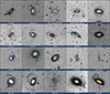 |
Fig. 1. Examples of stellar stream images from SSLS (Martínez-Delgado 2024). The cutout angular sizes vary between 3 × 3 and 10 × 10 arcmin. The images include characteristic examples of morphological types, such as great circle (NGC 1121, UGC 8717, and 2MASXJ01463936+3206305) umbrella/shell (NGC 922 and NGC 681), and great plume (ESO 199-012), as well as those of more complex, composite morphological types (IC 169 and NGC 1097). |
In this paper, we compare the stellar streams in a sample of galaxies observed by the DES survey with streams in mock images derived from the simulations listed above for a matched sample of hosts. We compare the detection frequency and photometric characteristics measured in both samples and discuss the results. In Section 2 we introduce the main characteristics of the cosmological simulations. The selection of the halos from the simulations to be analysed is presented in Section 3. Section 4 is devoted to the process of generating mock images. In Section 5, we present the predicted detectability of streams at different surface brightness limits. In Section 6, we present the results of the photometry measurements in the mock images. The results of the comparison are discussed in Section 7 and the summary, conclusions, and outlook are given in Section 8.
2. Cosmological simulations
This work makes use of several different cosmological simulations. An overview of the available cosmological simulations, as well as the underlying tools and modelling paradigms, can be found in Vogelsberger et al. (2020) and are also part of the AGORA collaboration (Roca-Fàbrega et al. 2024). For our work, we selected three simulation sets, each belonging to one of the broad categories in which the cosmological simulations are classified at the highest level:
-
Volume simulations produce large, statistically complete samples of galaxies, but they are typically not resolved on spatial scales smaller than ∼100 pc. Physical processes on scales smaller than the explicit hydrodynamical scheme, such as star formation and feedback, are incorporated via semi-analytical ‘sub-grid’ models.
-
Zoom-in simulations produce smaller samples of galaxies with a higher spatial and mass resolution and, therefor, model baryonic processes on smaller scales.
-
Semi-analytical simulations are the result of a combination of numerical dark matter-only simulations and analytic models for the prescription of baryonic physics. They are computationally much more efficient than the above categories, at the cost of self-consistency in the dynamics of the baryonic component.
For our comparison with the observational data, we chose one state-of-the-art simulation suite of each of the types listed above.
2.1. Copernicus Complexio
The Copernicus Complexio (COCO; Hellwing et al. 2016) is a ΛCDM cosmological N-body simulation post-processed with a semi-analytic galaxy formation model and the Stellar Tags in N-Body Galaxy Simulations (STINGS) particle tagging technique (Cooper et al. 2010, 2017). COCO provides both high mass resolution and an approximate analogue of the Local Volume (a high-resolution spherical region of radius ∼25 Mpc, with a density that is slightly lower than the cosmic mean, embedded in a lower-resolution box of 100 Mpc/side). The specific characteristics of the COCO simulations are listed in Table 1. The Galform semi-analytic model of Lacey et al. (2016) was used to predict the evolution of the baryonic component in each dark matter halo. This is a forward model, in which the exchange of mass between the circumgalactic gas, the cold ISM, stars and central supermassive black holes is tracked by a coupled network of differential equations describing processes such as radiative cooling, star formation, recycling, and supernova feedback. Merger trees extracted from the simulation provide boundary conditions for these equations in terms of the growth rates of individual dark matter halos. The model is calibrated to a range of low- and high-redshift observables, including optical and near-IR luminosity functions, the HI mass function, and the relationship between the masses of bulges mass and central supermassive black holes. In addition to these calibrations, it is relevant to this work that predictions for the luminosity function of low-mass galaxies in Lacey et al. (2016) are in good agreement with the observations, including those in the regime of the MW satellites (e.g. Bose et al. 2018).
After the COCO merger trees have been processed with the Lacey et al. model, the six-dimensional (6D) phase space of each single-age stellar population formed is mapped to an individual subset of dark matter particles using the STINGS technique. The resulting simulated galaxy population2 is described in detail by Cooper et al. (2025). COCO is complementary to the hydrodynamical TNG simulations (described below); it provides predictions that are sufficiently calibrated to the stellar mass-halo mass relation inferred from abundance matching, as well as to the observed relation between galaxy size and stellar mass, both of which have a direct influence on the counts and luminosity of tidal features around hosts of a given virial mass. Cooper et al. (2025) demonstrated that the COCO model predictions are in good agreement with the available data on accreted stellar mass fractions and surface density profiles in the LSB regime.
It is still unclear to what extent galactic gravitational potentials are modified by gas dynamical processes (e.g. through the formation of massive gaseous and stellar disks or through feedback-induced transformations of satellite density profiles) and how such modifications affect the disruption of satellite galaxies. Since both COCO and TNG are adequately calibrated to the observed galaxy stellar mass function, comparisons between these two models can explore these baryonic effects: galactic potentials and tidal stripping in TNG may be influenced by the gravitation of the baryons, but by construction, this is not the case in COCO (see e.g. Cooper et al. 2017, for an extensive discussion of comparisons between hydrodynamical and particle tagging simulations).
2.2. TNG50
IllustrisTNG is a suite of large volume, cosmological, magnetohydrodynamical simulations run with the moving-mesh code AREPO (Springel 2010) and with publicly available data (Nelson et al. 2019a). One such run, at the highest resolution, is known as TNG50-1, or simply TNG50 (Pillepich et al. 2019; Nelson et al. 2019b). This is the run used in this work, with its key characteristics listed in Table 1.
Characteristics of the cosmological simulations used in this work.
The TNG50 simulation includes a comprehensive model for galaxy formation physics, which is able to realistically follow the formation and evolution of galaxies across cosmic time (Weinberger et al. 2017; Pillepich et al. 2018). TNG50 self-consistently solves the coupled evolution of dark matter, cosmic gas, luminous stars, and supermassive black-holes from a starting redshift of z = 127 to the present day, z = 0. In this work, we focus on the snapshots at z < 0.02.
The TNG50 simulation3 delivers 198 MW/M31 analogues, namely, disk galaxies with stellar mass in the range of M⋆ = 1010.5 − 11.2 M⊙, along with a MW-like stellar morphology and a cosmological environment at z = 0 (Pillepich et al. 2024). The mass resolution is 8.5 × 10⁴ M⊙ for baryonic particles and 4.5 × 10⁵ M⊙ for dark matter particles. The average spatial resolution in the star-forming regions is ∼150 pc. The simulation features a large range of galaxy and halo properties, as well as past histories and the simulated galaxies display global properties that are consistent with those measured for the MW and Andromeda.
Regarding applications, TNG50 is widely used for scientific studies on diverse aspects of galaxy formation and evolution. A list of 12 ongoing applications is captured in Table 2 of Pillepich et al. (2024). The aspects that are relevant for this paper include the abundance and properties of the current satellites of MW/Andromeda-like galaxies in the TNG50 simulations yielded results that are consistent with the observations (Engler et al. 2021, 2023). The TNG50 simulation has been used for the study of dwarf galaxy accretion in the MW in Folsom et al. (2025), which is particularly relevant to our application.
2.3. Auriga
The Auriga simulations (Grand et al. 2017, 2024) are a set of cosmological zoom-in magnetohydrodynamical simulations also carried out with the AREPO code. Auriga re-simulates at higher resolution a sample of halos selected by the EAGLE project (Schaye et al. 2015) and implements models for black hole (BH) accretion and feedback, stellar feedback, stellar evolution, chemical evolution, metallicity-dependent cooling, star formation, and magnetic fields, as reported in Grand et al. (2017).
From the simulations available on the Auriga portal4 we used all 30 halos in the Original/4 series. These simulations have a baryonic (dark matter) mass resolution of 5 × 10⁴ (3 × 10⁵) and, thus, a slightly higher mass particle resolution than the TNG50 simulations, offering an additional valid comparison with observations and smooth particle hydrodynamics (SPH) modelling. Higher resolution Auriga simulations exist (see discussion in Section 7), but with a much lower number of halos, which would render our analysis statistically non-representative. The key characteristics of the Auriga simulations applied to our work are listed in Table 1.
The Auriga simulations have been extensively used for studying accretion in MW-like galaxies, including tidal streams, leading to recent publications (Vera-Casanova et al. 2022; Shipp et al. 2024; Riley et al. 2024; Pu et al. 2025). This allows for a comparison with our findings from the same simulations, as presented in Section 7. In addition, Auriga and TNG50 have been applied to the study of satellites undergoing ram pressure stripping (RPS) during their infall on MW- analogues selected in the SAGA study. Comparisons of both simulations with observations of the Canada–France–Hawaii Telescope and the Jansky Very Large Array show a consistent global behaviour (Jones et al. 2024).
3. Halo selection
To allow for a consistent comparison between the cosmological simulations and the DES image sample, we selected samples of simulated halos in a comparable range of both stellar mass and halo mass. To determine the range of host stellar mass in the DES sample, we constructed an empirical relation between the absolute magnitude of the galaxies in the B-band, MB, available from the HyperLeda database5 (Makarov et al. 2014), and their stellar mass, M⋆, as determined by the Spitzer Survey of Stellar Structure in Galaxies (S4G, Sheth et al. 2010). We find the following relation:
 (1)
(1)
As shown in Figure 2, this empirical relation is linear over the magnitude range of the DES host sample, with small scatter; that is, generally less than 0.2log10(M*/M⊙) bar a few outliers.
 |
Fig. 2. Stellar mass versus B-band absolute magnitude from the Spitzer S4G catalogue. The red line represents the empirical correlation in Equation (1). |
The histogram in Figure 3 shows the stellar mass distribution of the DES sample and of the selected halos in the COCO, TNG50, and Auriga simulations. The average stellar mass of the DES sample is log10M⋆/M⊙ = 10.00 and a standard deviation of σ = 0.38. While the average of the distributions is not the same, there is sufficient overlap between the DES sample stellar mass range and the stellar mass range of the simulated halos selected for the comparison. Figure 4 shows the halo massdistribution of the selected halos in the COCO, TNG50, and Auriga simulations. Here, all the simulations overlap and the average values are close to one another. In this stellar mass range, COCO galaxies occupy a broader range of halo masses than the TNG50 galaxies.
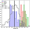 |
Fig. 3. Histogram of log10M⋆ for the observed DES sample of 689 galaxies (grey) and simulated galaxy samples from COCO (108 host galaxies, in blue) TNG50 (60 host galaxies, in red), and Auriga (30 host galaxies, in green). The black vertical line shows the average of the DES sample (log10M⋆/M⊙ = 10.00) and the dark grey vertical lines the ±1σ range around that average, [9.62, 10.38]. The light grey vertical line shows the average of the DES sample +2σ = 10.76. The maximum value of each histogram has been re-scaled to 1 for this comparison. |
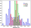 |
Fig. 4. Histogram of the log10 halo mass. Colours correspond to simulation sets, as shown in the legend and Figure 3. The maximum value of each histogram was re-scaled to 1 for this comparison. |
Figure 5 shows the stellar mass versus the halo mass for the selected sample of galaxies in the COCO, TNG50, and Auriga simulations, compared with the empirical correlation by Moster et al. (2018) ±2σ. The horizontal lines indicate the mean value, mean value −1σ and mean value +2σ for the DES galaxy sample stellar mass distribution. While TNG50 galaxies are within Moster’s correlation ±2σ, some Auriga galaxies seem to be slightly above the = 2σ correlation range. COCO shows a larger scatter of stellar mass in the region above log10Mhalo/M⊙ and has a rather sparse sample of galaxies around the MW region. These COCO simulation characteristics are discussed in depth in Cooper et al. (2025).
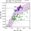 |
Fig. 5. Stellar mass versus halo mass for the selected sample of galaxies in the COCO, TNG50, and Auriga simulations compared with the empirical correlation by Moster et al. (2018) ±2σ. The horizontal lines indicate the DES galaxy sample stellar mass distribution: mean value (dotted line); mean value −1σ (lower dashed line) and mean value +2σ (upper dashed line). The yellow star represents the MW. |
4. Mock images
To compare the predictions of cosmological simulations with the observations from the DES sample, we generated mock images from snapshots of the simulations described in Section 2 in the redshift range 0 < z < 0.02. The continuous stellar mass density field in all these simulations is represented by discrete tracers, called star particles6. The stellar mass associated with each star particle corresponds to a stellar population with a single age and metallicity. The assumption of a SSP for mass particles can be considered as adequate for our work, based on the findings in Grand et al. (2017) where the simulated galaxy stellar populations were compared to observations. They report that the distribution of simulated galaxies is centred around a mean stellar age of ∼5–7 Gyr, which is roughly the age range expected for galaxies like the MW from the observations of Gallazzi et al. (2005). Also, the rightmost panel of their Figure 20 shows that the metallicities of the simulated galaxies reproduce the observed metallicity of MW-like galaxies. As in any N-body realization of a density field, each particle notionally corresponds to an irregular volume of phase space centred on the location of the particle.
We applied the following transformations to the properties of the star particles from the simulation snapshots in order to recover the observables that can be identified in real images:
-
Expansion of the discrete star particles into an approximation of the implied continuous 3D of stellar mass distribution, via a convolution with an adaptive smoothing kernel.
-
Projection of the continuous distribution of stellar mass into a 2D plane. The orientation of the central galaxy relative to the observer’s line of sight is a parameter of our method, and can be either random or specific (for example, to view the galaxy face-on or edge-on).
-
Conversion of stellar mass density to luminosity density, via a convolution of an SED appropriate to the age and metallicity of each particle with a specific photometric bandpass.
We used the open source tool pNbody7 (Revaz 2013) to produce mock images by implementing the transformations above. Figure 6 shows, as an example, the r-band surface brightness map produced by processing one of the COCO galaxies with pNbody. The contour lines identify the isophotes for an intuitive view of the possible LSB structures present in the image. We carried out tests to assess the robustness of the resulting mock images to variations in the pNbody configuration parameters for generating mock images with the DECam instrument.
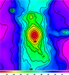 |
Fig. 6. Example of a surface brightness map produced with pNbody. The black contours mark the isophotes of surface brightness, starting with 20 mag arcsec−2 in the centre of the host galaxy and separated by increments of 1 mag arcsec−2. |
To assess the impact of the host distance on the detectability of streams, we generated mock images at different distances (50, 70, and 90 Mpc), covering the distance range of the observed DES sample hosts with their streams, which ranges from 40 to 100 Mpc. Although the surface brightness is independent of the distance, the distance has an impact on the S/N at pixel level that may, in turn, impact the observability. However, as expected, this small relative difference in distance does not show a noticeable difference in the visual perception of the images. Changing the distance within the DES galaxy sample range does not noticeably influence the detectability of streams; therefore, we generated mock images from surface brightness maps with host galaxies at a distance of 70 Mpc from the Sun, as representative distance for the DES galaxy sample.
For the expansion (smoothing) step, we distributed the luminosity (flux) of each particle over the image pixels by convolution with a Gaussian kernel. The scale of this kernel, h, which we refer to as the smoothing scale, is set to a parametrized multiple of the root-mean-square average distance to the 16th-nearest star particle neighbour, h16. It therefore adapts to the local star particle density. The logic for setting h is broadly similar to that used to determine the kernel scale in a smoothed particle hydrodynamics calculation. However, the smoothing in our case only serves to interpolate between the original particles and does not have any physical significance. It is therefore somewhat arbitrary; our method reflects a balance between smoothing sufficiently to reduce the visual impression of a discrete particle distribution, while preserving the small-scale features.
Figure 7 shows mock images of the same three galaxies (left to right) with kernels of scale h = 0.6 h16 (top row) and h = 0.3 h16 (bottom row). Over this range (with the DESI pixel scale) the bulk of the particle granularity in the image is removed, but nature, extent and surface brightness of tidal features relevant to our subsequent visual inspection (see Section 5) are not noticeably different.
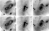 |
Fig. 7. Comparison of smoothing methods. The top panels show the surface brightness map of three different halos generated with a smoothing length up to the 16th neighbour multiplied by the factor 0.6. The bottom panels show the surface brightness maps of the same halos but applying a factor of 0.3 to the smoothing length to the 16th neighbour. |
We use the mock images (i) to assess the detectability of streams over a range of surface brightness limits and (ii) to measure the photometry of the streams that would be detectable at the surface brightness limit of the DES observations. To follow the same process of stellar stream detection by visual inspection as with real images, we transformed the surface brightness maps into counts images. Then we added background noise to the images, which depends on the type of analysis to be carried out.
In order to assess the detectability of the streams under different image depths, a simple realization of background noise was added to the images, as flat Gaussian noise with variable amplitude. This gives us the flexibility to emulate different surface brightness limits in an easy way; we choose limits between 25 and 34 mag arcsec−2 in intervals of 1 mag arcsec−2. For this purpose we used the state-of-the-art GNU Astronomy Utilities (Gnuastro)8 software (Akhlaghi 2019a,b; Akhlaghi & Ichikawa 2015).
To asses the impact of the smoothing length on the detection of a possible stream in the mock images by visual inspection, we examined count images with different choices of smoothing length, after adding background noise corresponding to a surface brightness limit of 29 mag arcsec−2. Figure 8 shows this test for smoothing lengths h = 0.6 h16, h = 0.3 h16 and an alternative smoothing scheme in which h is instead set to the absolute distance to the 5th nearest neighbour. Again, regarding stream detection by visual inspection, we find no significant difference between the images. We therefore adopt a smoothing scale of h = 0.6 h16.
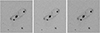 |
Fig. 8. Comparison of smoothing methods. Images generated from the surface brightness maps, by transforming the surface brightness to counts, and adding background noise to emulate a surface brightness limit of 29 mag arcsec−2. The left and centre images correspond to a smoothing length equal to the distances to the 16th nearest neighbour multiplied by a factor of 0.3 (left) and a factor of 0.6 (centre). The right panel shows the image produced with a different smoothing length, considering the distance to the fifth neighbour. |
To measure photometric properties of the mock images and compare the results with those of the DES sample, we add a more realistic sky background to the mock images. We first extract the sky background from selected real DES sample images, removing the central galaxy and replace it with a real sky background from an area of the same image without significant point sources. The image from which we extracted this fiducial background image was selected according to the following criteria: (i) the central galaxy should be edge-on, in order to minimise its area of influence on the image; (ii) the image should have no stream detection, in order not to interfere with the synthetic halo image; and (iii) the image should have an r-band surface brightness limit representative of the DES sample. The selected image had a surface brightness limit of 28.65 mag arcsec−2. The fiducial sky background extracted from this image, as above, was then superimposed onto the mock images generated directly from the surface brightness maps, that have only a central galaxy andpossibly other accompanying galaxies but no sky background, creating an image with a synthetic central galaxy and a real DES background.
We use Gnuastro to replace the central galaxy and its surroundings with a section of the same image extracted from a region without bright sources. The size and orientation of the ellipsoidal mask is such that covers the area of influence of the central galaxy in its surroundings; namely, it reaches up to the point where the surface brightness profile flattens.
Figure 9 shows examples of TNG50 and COCO mock images with streams around the central galaxies. Panels B show images to which we added the sky background of a real DES image with a surface brightness limit of 28.65 mag arcsec−2. We compare these images to those in panels A, to which we added an artificial Gaussian sky background equivalent to the same surface brightness limit. The streams, though faint, can be clearly appreciated in the images with real DES background and, although they are more obvious in the image with artificial background, their appearance is consistent in both images. Consequently, adding a synthetic background to the mock images does not seem to impact significantly the detection of streams by means of visual inspection with respect to the real background in this surface brightness limit regime. This method is very efficient to emulate different levels of surface brightness limit and we adopt it in this work to assess the detectability of streams at those levels currently not achieved in available surveys. However, we acknowledge that for much fainter surface brightness limits, this method provides only an approximation as the confusion of sources and possibly cirri will become much more significant and the difference between the synthetic background and the real background will increase.
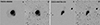 |
Fig. 9. Comparison of mock images with simulated and real DES sky background: examples of a TNG50 (left) and a COCO (right) simulated galaxy with stream stacked with a real DES sky background (panels B), and with artificial flat background (panels A) both having the same surface brightness limit of 28.65 [mag arcsec−2]. |
5. Stream detection
In this section, we analyse the detectability of tidal streams under different image depths on the basis of mock images. At present, there is no effective automatic method for detecting tidal streams, although this is an important subject of current research. Therefore, detectability is based here on the method that combines visual inspection and image analysis tools, as discussed in Section 1. This is the method applied to the detection of streams in real images, as presented in Miró-Carretero et al. (2024) and that has been the basis for generating the stream catalogue presented there.
The analysis was done on the basis of the r-band images. We chose this band as it has been used in other relevant observational studies on tidal features (Miskolczi et al. 2011; Morales et al. 2018; Bílek et al. 2020; Sola et al. 2022; Skryabina et al. 2024), thus allowing for a comparison of results across different studies. In the mock images, the SDSS r-filter produces brighter measurements of the stream than the SDSS g-filter, in agreement with the observations. Depending on the region in the image this difference can be up to ∼0.6 mag arcsec−2.
We transformed the surface brightness maps into images with counts and generated mock images by adding sky background corresponding to 10 levels of surface brightness limit between 25 and 34 mag arcsec−2 (see Section 4). As we increase the depth of the image (apply a lower background noise level to the image, corresponding to a fainter surface brightness limit), streams become more visible and can be detected by visual inspection, as illustrated in Figures A.1, A.2, and A.3.
We inspected the resulting mock images and for each host galaxy, the surface brightness limit at which a stream could be visually detected for the first time was identified and noted. The inspection was carried out on the image FITS-format files, displayed with the SAO DS9 tool. As for the inspection of the observational images, suitable colour, scale, and analysis block level options were selected to improve the perception. The curve corresponds to detections for which we have a reasonable level of confidence that are streams; namely, the morphology is typical of streams we have observed in real images. When we detected a LSB feature but still had doubts about whether that LSB feature constitutes a stream, we took the conservative approach of not counting it towards the results represented in the figure. We took into account the fact that the smooth background added to the image makes streams easier to detect in comparison with the real background of the DES sample images. Thus, we reported one level fainter of the surface brightness limit, when the stream cannot be clearly distinguished by visual inspection at a certain surface brightness limit level.
5.1. Stellar streams in the COCO simulation
For comparison with the DES sample, we first selected a sample of simulated COCO halos containing central galaxies with stellar mass in the range within the DES stellar sample average ±1σ, that is, between 4.17 × 10⁹ M⊙ (log10M⋆/M⊙ = 9.62) and 2.4 × 10¹⁰ M⊙ (log10M⋆/M⊙ = 10.38). To be able to compare also with the other simulations containing more massive host galaxies, we then extended the selected sample of simulated COCO halos to contain central galaxies with stellar mass corresponding to the DES host sample average stellar mass value +1σ and +2σ (log10M⋆/M⊙ = 10.76) and retained this sample for the stream detectability analysis.
For the COCO simulations, 108 halos have been selected with central galaxy stellar masses overlapping with 70% of the DES sample with streams, see Figure 3. This yields ∼1000 images for visual inspection, taking into account that for each surface brightness map, ten mock images were generated: one for each of the surface brightness limit considered.
The result is a curve indicating the percentage of galaxies with detected streams within the COCO halo sample as a function of the image depth, that is, as a function of the image surface brightness limit. This is depicted in Figure 10. The curve follows an approximately linear trend between surface brightness limits of 26 and 34 mag arcsec−2, with a 12.5% increase in streams detected per 1 mag arcsec−2 increase in surface brightness limit. In 97% of the mock images, we detect by visual inspection what we consider to be (part of) a stream up to a SB limit of 34 mag arcsec−2. However, we estimate that only 89% of such faint structures could actually be measured with a reasonable level of error in real images.
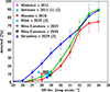 |
Fig. 10. Stellar stream detection rate, i.e. percentage of galaxies for which at least one stream could be detected as a function of the image surface brightness limit. Continuous lines represent the results for the TNG50 (red), COCO (blue) and AURIGA (green) simulations, with error bars showing the Poisson confidence interval. The plot also shows the results of observational stream surveys from the literature, discussed in Section 7.1. (1) The calculation of the SB limit follows a different method than the one applied in this work. (2) The detection rate has been derived for all LSB features, including streams. For the DES sample (black square symbol), the x and y dimensions of the symbol indicate the dispersion in surface brightness limit of the DES sample and the dispersion in the detection rate according to a binomial distribution, respectively, see Miró-Carretero et al. (2024). |
Regarding the stream morphology, in the COCO sample, at SB limit 28–29 arcsec−2, around 70–80% of the detected streams are shells – a segment of the wider morphology class known as umbrella, see stream morphology classification in Miró-Carretero et al. (2024) – while at SB limit 34 arcsec−2 around 80–90% of the detected streams are shells, with only 2–3% of the streams displaying a circular morphology.
We investigated a possible correlation between the surface brightness limit at which streams are detected and the host galaxy stellar mass. In particular, we analysed whether more massive host galaxies show streams at a lower (brighter) surface brightness limit. Figure 11 shows the stellar mass distribution for the galaxies identified as hosting streams versus the surface brightness limit at which those streams have been detected. No correlation is evident.
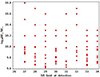 |
Fig. 11. Plot shows the log10M⋆/M⊙ distribution of the COCO halos vs the surface brightness limit at which their streams are detected. |
5.2. Stellar streams in the TNG50 simulation
We generated surface brightness maps from the TNG50 simulation for 60 halos. 40 of these have central galaxies in the stellar mass range between between 3.02 × 10¹⁰ M⊙ (log10M⋆/M⊙ = 10.48) and 5.73 × 10¹⁰ M⊙ (log10M⋆/M⊙ = 10.76), corresponding to the range of stellar mass between the average value of the DES sample +1σ and +2σ. In order to compare with MW-like galaxies (such as those in the Auriga simulations) we selected 20 additional halos in an extension of the stellar mass range to 8.0 × 10¹⁰ M⊙ (log10M⋆/M⊙ = 10.9), see Section 3 for details. We visually inspected the resulting ∼600 images and for each halo and host galaxy, the surface brightness limit at which a streams could first be visually appreciated was identified and noted.
Figure 10 shows the resulting curve indicating the percentage of galaxies with detected streams within the TNG50 halo sample as a function of the image surface brightness limit. The curve shows a steep gradient between SB limit = 30 and SB limit = 32 mag arcsec−2, of about 25% increase in streams detected per 1 mag arcsec−2 increase in surface brightness limit. In ∼70% of the mock images a (part of a) stream can be detected by visual inspection at a SB limit of 34 mag arcsec−2. The detection percentage level resulting from inspection of the TNG50 mock images at a SB limit of 28.65 mag arcsec−2 (the SB limit value corresponding to the average SB limit for the DES sample in the r band) is between 3% and 10% (corresponding to the SB limit values for 28 and 29 mag arcsec−2 in the curve, respectively).
To assess the dependency of the detection rate for a certain SB limit on the host stellar mass, we compared the detectability curve obtained for 40 halos in the stellar mass range between log10M⋆/M⊙ = 10.48 and log10M⋆/M⊙ = 10.76 with the one obtained for 60 halos in an extended stellar mass range up to log10M⋆/M⊙ = 10.9. As can be seen in Figure 12, both curves are very similar, the one for the extended mass range appearing smoother, due to the increased population of galaxies included. This seems to reinforce the speculation made in Section 5.1 using COCO simulations that the stellar mass of the host galaxy does not noticeably influence the brightness of the streams around it. The morphology analysis shows 20–43% of shells (part of the cosmological umbrella/shell class) and 10–16% circular shapes, some showing a clear loop around the host.
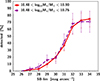 |
Fig. 12. Stellar streams detection rate as a function of the image surface brightness limit for the TNG50 simulation. The percentage of the streams detected by visual inspection is plotted versus the surface brightness limit at which such detection was possible. The solid line corresponds to a stellar mass range of log10M⋆/M⊙ = 10.48 and log10M⋆/M⊙ = 10.76, while the dashed line corresponds to an extended mass range up to log10M⋆/M⊙ = 10.9. |
5.3. Stellar streams in the Auriga simulation
We had access to 30 Auriga zoom simulations of MW-mass halos at z < 0.02. Since this sample may not be statistically representative, and in order to compare with the COCO and TNG50 simulations, two surface brightness maps have been generated from each halo, taking two orthogonal axes of the simulation coordinate system as lines of sight. None of the axes are aligned with face-on or edge-on direction, so that overall the orientation of the galaxies is random. This process results in 60 surface brightness maps, each of which is complemented with sky backgrounds as explained above, thus yielding 600 mock images in total. Examples of halos with streams of different morphology can be seen in Figure A.3.
Figure 10 shows the detection rate curve obtained for Auriga from visual inspection of the mock images, together with those obtained for COCO and TNG50, and the observational results of the DES sample. The figure shows the percentage of the sample for which at least one stream is detected for each of the 10 surface brightness limit levels analysed. Two of the halos (Au11 and Au30) seem to show an ongoing major merger between two galaxies of similar apparent size, clearly visible at a surface brightness limit of 26 and 27 mag arcsec−2, respectively. These two halos have been discarded, because we are looking for remnants of minor mergers only. LSB structures that could appear similar to streams at fainter surface brightness limits in these halos are not accounted for in the detectability curve, as it cannot be ascertained that these features are not the result of the major merger.
The curve shows that there are no stream detections at a SB limit 26 mag arcsec−2 or brighter. Between 26 and 29 mag arcsec−2 there is an increase in detections with a gradient of around 4% detection rate per mag arcsec−2 the SB limit, reaching ∼12% detection rate at 29 mag arcsec−2. Between 29 and 31 mag arcsec−2 the gradient is about 4 times steeper, reaching ∼34% detection rate at 31 mag arcsec−2. The gradient increases again to ∼25% per mag arcsec−2 increase in the SB limit between 31 and 32 mag arcsec−2 reaching ∼65% detection rate at this SB limit. Beyond this value, the gradient flattens. We detect streams by visual inspection with a reasonable level of confidence in 95% of the mock images up to a SB limit of 34 mag arcsec−2. The percentage of streams detected in the AURIGA sample at a SB limit corresponding to the average SB limit for the DES sample in the r band (28.65 mag arcsec−2) is between 8% and 13% (corresponding to the SB limit values for 28 and 29 mag arcsec−2 in the curve, respectively).
The morphology analysis yields 41–62% shells and 11–24% circular shapes. However, the observed stream morphology is strongly dependent on the line-of-sight from which the streams is observed (Youdong et al., in prep.). As an example, Figure 13 shows halos Au14 and Au29 seen from two different lines of sight. As can be appreciated in the images, looking at the same halo from these two different perspectives would suggest a different morphological classification.
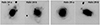 |
Fig. 13. Example of the impact of the line-of-sight on morphology classification. Left: Two views of Auriga halo 14 at a surface brightness limit of 31 mag arcsec−2 from different line of sight. Right: Same views for Auriga halo 29 at a surface brightness limit of 31 mag arcsec−2. |
Percentages of the principal stream morphologies in observation and simulations.
6. Stream photometry
We carried out a photometric analysis of the mock images generated from cosmological simulations through the process described in Section 4. We present here the results of the characterisation and photometric analysis of the mock imagesgenerated from the COCO, TNG50, and Auriga simulations and compare them with the ones obtained from the DES observations sample reported in Miró-Carretero et al. (2024)). To measure photometry parameters such as surface brightness and colours on the mock images the corresponding surface brightness maps have been generated for the SDSS r,g and z filters and transformed into counts images.
To compare the photometry of images with a similar surface brightness limit, the output of the simulations has been enhanced by superimposing a real DES sky background selected to have a surface brightness limit corresponding to the average surface brightness limit of the DES image sample with streams, namely 28.65 mag arcsec−2 (see Section 4). As a result, only those mock images have been selected for the comparison, in which a stream was detected at a surface brightness limit of ≲28.65 This resulted in 21 mock images from the COCO simulation, 8 mock images from the TNG50 simulation, and 6 mock images from the Auriga simulation. Their photometry parameters are compared against those from 63 images of the DES sample with streams. This means that a statistically sound comparison is not possible; nevertheless, the comparison is useful to see whether the cosmological simulations can reproduce real photometric observations, which requires realistic predictions of particle metallicity and age. These, in turn, are the result of the modelling of the physical processes involved.
The comparison between the mock images photometry and the observations from the DES galaxy sample is carried out on the basis of the average stream surface brightness, average stream (g − r)0 colour as well as the average distance of stream to the host centre. The resulting histograms are shown inFigures 14, 15, and 16.
 |
Fig. 14. Histogram of the distribution of average surface brightness measured on the stream for the g (top) r (centre) and z (bottom) bands. |
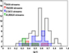 |
Fig. 15. Histogram of the distribution of average (g − r)0 colour measured on the stream. |
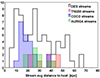 |
Fig. 16. Histogram of the distribution of average distance of the streams to the centre of the host galaxy. |
7. Discussion
We go on to compare the predictions of the cosmological simulations with one another and with the observational data regarding frequency, detectability, and morphology of streams as well as their photometric properties. Looking at Figure 10, the cosmological simulations all seem to predict that, for a surface brightness limit of 32 mag arcsec−2, almost 70% of galaxies in the mass range we study have one or more detectable streams.
However, the simulations show discrepancies with one another regarding detection rates for surface brightness limits brighter than 32 mag arcsec−2. In particular, the two hydrodynamical simulations, TNG50 and Auriga, agree well with each other but predict a lower detectability rate than COCO. For limits fainter than 32 mag arcsec−2, however, TNG50 has a lower detection rate than COCO and Auriga (which agree well with each other, in this regime). The simulations also show discrepancies with one another regarding the morphology of the streams detected, as will be discussed further down in this section.
The small differences in the stellar mass ranges of the samples of galaxies drawn from the three simulations (see Figure 3) do not seem to play an important role in stream detectability for the range of stellar masses analysed in this work, as discussed in Section 5.1. We therefore speculate that these differences can be attributed mainly to the treatment of baryon physics in the simulations (all the simulations use the same N-body treatment of gravitational dynamics and very similar cosmological parameters). Pinpointing specific explanations for these differences will require an in-depth analysis, outside of the scope of this work. However, since the most striking difference concerns the apparently greater number of relatively brighter streams detectable in the COCO particle tagging models, compared to the two hydrodynamical simulations, we speculate on why differences in the dynamical treatment of the baryons may give rise to this result.
As discussed in Cooper et al. (2017), when comparing particle tagging simulations with hydrodynamical methods, even with identical initial conditions, it can be difficult to separate effects due to the dynamical approximation of particle tagging from the effects of different star formation models. In our case, the IllustrisTNG and COCO models have both been calibrated to observations of the galaxy mass and luminosity functions at z = 0 (in the case of COCO via the semi-analytic model of Lacey et al. 2016), as well as other low-redshift data, notably the galaxy size–mass relation. The fundamental relationship between stellar mass and virial mass in both simulations agrees well with (for example) that inferred from galaxy abundance matching. Although the typical star formation histories of host galaxies in our sample, and their stream progenitors, may still differ in detail between the two simulations, we expect that they are broadly similar. This makes it more likely (although by no means certain) that the differences we observe are related to dynamical factors, rather than differences in how stars populate dark matter halos.
Two particularly relevant dynamical factors are neglected (by construction) in particle tagging models. First, the gravitational potentials of stream progenitors can be altered by the inflow and outflow of baryons associated with cooling and feedback; this may make satellites either more or less resilient to tidal stripping, depending on whether baryonic processes produce density cores or density cusps. Second, stars (and gas) could make a significant contribution to the central potential of the host halo, in particular through the formation of a massive baryonic disk.
Cooper et al. (2017) explore the consequences of neglecting these factors when predicting satellite disruption (and hence stream and stellar halo formation) in particle tagging models. In the hydrodynamical model used in that work, massive satellites were found to disrupt somewhat earlier than realizations of the same systems in a particle tagging model9. This could explain why more streams are visible at surface brightness limits of ≲28 mag arcsec−2 in COCO compared to IllustrisTNG; if satellites are disrupted earlier in IllustrisTNG, their streams may have more time to phase mix, lowering their surface brightness. A similar argument could also explain the greater abundance of shells detected in COCO. Shells originate from satellites on radial orbits (Newberg & Carlin 2016). The relative fraction of radial and circular orbits may differ between IllustrisTNG and COCO, because the evolution of the progenitor’s orbit during pericentric passages (due to exchange of angular momentum with the host) may be significantly different with and without a massive baryonic disk. Valenzuela & Remus (2024) explore a related effect by studying the relation between the rotation of the hosts and the presence and morphology of tidal features. One of the conclusions of that work is that shells appear more frequently in slow rotating hosts than in fast rotating hosts. This hypothesis could be tested in future work. More generally, further exploration of these differences particle tagging and hydrodynamical simulations could help to understand how observations of streams can constrain the nature of the gravitational potentials of stream progenitors and their host galaxies.
Turning to comparisons between the simulations and the observational data, 8.7 ± 1.1% of galaxies in the DES sample have detectable streams at an average r-band surface brightness limit of 28.65 mag arcsec−2. This seems to match very well with the predictions of TNG50 and Auriga, and is lower than the prediction from COCO.
Stream morphology is not an observable that can be used reliably to constrain simulations, because it is strongly dependent on the line of sight along which the stream is observed. Nevertheless, comparison of the fraction of streams with differentmorphologies is interesting because it could be related to the same dynamical differences between simulations methods that give rise to differences in stream abundance. 20–43% of streams in the TNG50 sample are shells, which is within the range found in the DES sample, and 10–16% have circular morphology, which is also not too far from the observations. As noted above, there is a significant discrepancy in the relative fractions of different stream morphologies between observations and the COCO simulations. In the COCO mock images, 70–90% of streams are identified as having an umbrella or shell morphology, while in the DES sample, only 27–38% of streams are identified as such. The COCO mock images show only 2–3% of streams with circular morphologies, compared to 21–35% in the DES images. Auriga predicts 41–62% of streams with umbrella/shell morphologies, significantly above the fraction in the DES sample, and 10–24% of stream with circular morphology, somewhat below the DES figures. Table 2 summarises the stream morphology findings for the different samples derived from the total number of streams detected. We note that more than one stream is detected in some of the halos. It is beyond the scope of this work to analyse the reasons for these discrepancies in stream morphology; as noted above, further works would be a valuable contribution to understanding the relationship between the observable properties of streams and the galaxy formation process as a whole.
Regarding the stream photometry measurements, the stream average surface brightness range in the COCO simulation matches generally well the observations in the DES stream sample, though the distribution is skewed towards the brighter end of the range (Figure 14). This is consistent with the abundance of shell-shaped streams, typically brighter than other stream morphologies, as confirmed by the observations. The range of the stream average surface brightness in the TNG50 simulation falls pretty much within the central region of the DES sample range. For the Auriga simulations, the surface brightness conforms well with the other simulations, through falls slightly on the brighter side of the DES sample. Due to the very small number of galaxies analysed for TNG50 and Auriga (8 and 6, respectively) in comparison with COCO and the DES sample (18 and 60, respectively) any detailed comparison is out of scope, however, it is reassuring to see that the range of the photometry parameters in the simulations overlap with one another and are within the range of the observational sample.
The stream (g − r)0 colour distribution of the COCO simulations also matches generally well the observations. The mean value of the COCO simulation distribution is 0.54 ± 0.12 mag, versus 0.57 ± 0.14 mag for the DES observations sample. However, the simulations are slightly skewed towards the blue end as can be seen in Figure 15. The TNG50 and Auriga simulation results, though not statistically significant, show a (g − r)0 colour distribution spanning almost the full range covered by the DES observations.
Consistent with the overabundance of shell stream morphology in the COCO simulations, the average distance of the streams to the host galaxy is between 10 and 30 kpc, thus covering the lower end of the DES sample distance range, see Figure 16. The streams from the TNG50 simulation are at an average distance between 20 and 50 kpc from the host centre, covering the central part of the distance range observed in the DES sample. This is very similar to the Auriga simulations that show distances between 15 and 45 kpc.
7.1. Comparison with previous work
In this section, we present a comparison with other observations of streams as far as reported in the literature. Miskolczi et al. (2011) reported a frequency of 6–19% at a SB limit of ∼27 mag arcsec−2. We considered the lowest value of 6% as the most reliable for maximising purity in the detection of streams (see Figure 10).
Atkinson et al. (2013) reported a LSB feature (a superset of tidal streams) detection frequency of 12–18% at an average SB limit of ∼27.7 mag arcsec−2 for the g-band. We note that the g-band in the DES sample is fainter in average than the r-band by ∼0.5 mag arcsec−2. It is also to be noted that the calculation of the SB limit in that paper is based on 1σ of the noise variation in apertures of 1.2 arcsec2 placed on empty regions of the images and, therefore, it differs from the one applied in this work [3σ, 100 arcsec2] that follows the standard proposed in Román et al. (2020). Morales et al. (2018) reports a frequency of ∼10% at a SB limit of 28 mag arcsec−2. Bílek et al. (2020) reports 15% of tidal features, including 5 ± 2% for streams and 5 ± 2% shells (which we consider together in our curve) at a SB limit of 28.5–29 mag arcsec−2 for the g-band. We note that the g-band in the DES sample is fainter in average as the r-band by ∼0.5 mag arcsec−2.
Sola et al. (2022) characterised the morphology of more than 350 LSB structures up to a distance of 42 Mpc through annotation of images from the Canada–France Imaging Survey (CFIS2) and the Mass Assembly of early-Type gaLAxies with their fine Structures survey (MATLAS, Duc 2020; Bílek et al. 2020). They obtained 84 annotations for streams and 260 for shells; however, from these figures alone, it is not possible to derive detectability figures for the brightest streams and shells, as there could be several of them in one image.
Miró-Carretero et al. (2023) reported on the search of stellar tidal streams in DESI Legacy Survey images of MW-like galaxies, at distances between 25 and 40 Mpc, from the SAGA II galaxy sample (Geha et al. 2017; Mao et al. 2021). Applying the same detection and characterisation methods as in this work, their statistical analysis yielded a stream detection frequency of 12.2 ± 2.4% at a SB limit of 28.40 mag arcsec−2.
Rutherford et al. (2024) used deep imaging from the Subaru-Hyper Suprime Cam Wide data to search for tidal features in massive [log10M⋆/M⊙ > 10] early-type galaxies (ETGs) in the SAMI Galaxy Survey. They report a tidal feature detection rate of 31 ± 2% at a surface brightness limit of 27 ± 0.5 mag arcsec−2 for the r-band. They calculated the surface brightness limit following the same approach as Atkinson et al. (2013), which is in contrast to our method [3σ, 100 arcsec2]. For comparison, our method applied to a test Subaru HSC image yielded a surface brightness limit of 29.79 mag arcsec−2.
Skryabina et al. (2024) presented the results of visual inspection of a sample of 838 edge-on galaxies using images from three surveys: SDSS Strip-82, Subaru HSC, and DESI (DECals, MzLS, and BASS). In total, 49 tidal features out of 838 images are reported, equivalent to a frequency of 5.8% at a SB limit of 28.60 mag arcsec−2. In that study, tidal features include also disc deformations and tidal tails, typical of major mergers. Also, a number of papers in the literature report the frequency of tidal features (including streams and shells) in cosmological simulations, as described below.
Martin et al. (2022) reported on detections of tidal features inspecting mock images produced using the NEWHORIZON cosmological simulations. Through the production of surface brightness maps at different surface brightness limits, they predicted the fraction of tidal features that can be expected to be detected at different levels of limiting surface brightness. In this study, tidal features comprise: (i) stellar streams; (ii) tidal tails; (iii) asymmetric stellar halos; (iv) shells; (v) tidal bridges; (vi) merger remnants; and (vii) double nuclei – of which only (i) and (iv) are clearly of an accreted nature. For a surface brightness limit of 35 mag arcsec−2, expert classifiers were able to identify specific tidal features in close to 100 per cent of galaxies (M⋆ > 109.5 M⊙), in agreement with our results. For the range of stellar mass of the DES sample, log10M⋆/M⊙ = 10, they reported a detection rate of ∼25% for streams and shells together at a surface brightness limit of 30 mag arcsec−2 in the r-band. The detection rate becomes 35% for a surface brightness limit of 31 mag arcsec−2. These figures match very well our predictions with Auriga and TNG50.
In Khalid et al. (2024), the results of identification and classification of tidal features in LSST-like mock images from cosmological simulations are reported. Four sets of hydrodynamical cosmological simulations are used: NewHorizons, EAGLE, IllustrisTNG, and Magneticum. The frequency of tidal features, expressed in fractions of the total number of images, is between 0.32 and 0.40 showing consistency across the different simulations. Tidal Features comprise streams and tails, shells, plumes, or asymmetric stellar halos and double nuclei. Looking only at streams and shells, the percentage of detections varies between 5–15% depending on the level of confidence, for a SB limit of 30.3 mag arcsec−2 in the r-band.
In Vera-Casanova et al. (2022), the authors reported the results of inspecting surface brightness maps generated from 30 Auriga cosmological simulations (Grand et al. 2017) of MW-like galaxies looking for the brightest streams. These simulations are the same as those that we applied in this work. They report that no streams have been detected in images with a surface brightness limit brighter than 25 mag arcsec−2 and that the stream detection frequency increases significantly between 28 and 29 mag arcsec−2. For a surface brightness limit of 28.50 mag arcsec−2 in the r-band, they reported a detection rate of ∼18–30%. This is higher than our results show with the same Auriga simulations and we believe the reason is the different pixel size of the mock images. While we used the pixel size of the DECam instrument, 0.262 arcsec, equivalent to 0.08 kpc at 70 Mpc distance, Vera-Casanova et al. (2022) used a pixel size of 1 kpc. This is relevant for the visual inspection of counts images, as it has an impact on the S/N per pixel and could account for a significant difference in the surface brightness limit at which the streams are detected. Rebinning the DECam images to a 1 kpc pixel size shows that this difference exceeds 2 mag arcsec−2.
In Shipp et al. (2024) and Riley et al. (2024) the authors analysed the impact of stellar mass resolution in the Auriga cosmological simulation on the disruption of dwarf satellites. To do that they traced back the accreted particles in the simulation to the halos where they originated, by inspecting the simulation snapshots and identifying the merger trees from redshift z = 0 to z = 127. They considered three states of particles: intact dwarfs, streams and phase-mixed and concluded that approximately 50–70% of progenitors in Auriga were in the process of actively disrupting. The sensitivity of the results to the mass particle resolution, which is most relevant for our work, is assessed by comparing the simulations with level 4 resolution (m⋆ = 5.4 × 10⁴, mDM = 2.9 × 10⁵ M⊙, the one used in our work) with levels 3 (m⋆ = 6.7 × 10³, mDM = 3.6 × 10⁴ M⊙) and 2 (m⋆ = 8.5 × 10², mDM = 4.6 × 10³ M⊙). They found consistency in the stellar morphology of the individual objects across the different resolution levels, although due to the limited number of simulations, in particular for levels 3 and 2 (6 and 1, respectively) these results cannot be considered as statistically meaningful. A relevant finding is that many of the Auriga simulations have stellar streams on orbits consistent with the MW dwarf galaxy streams (rperi ≤ 20 kpc, rapo ≤ 50 kpc) which is also consistent with our findings (see Figure 16). However, they did not analyse the detectability of the streams using mock images (which they left to a future work); therefore, a direct comparison of detectability for the different resolution levels is not possible.
Valenzuela & Remus (2024) used the Magneticum Box4 hydrodynamical cosmological simulations to detect tidal features (streams, shells, and tidal tails) and connected their morphology to the internal kinematics of their host galaxies. In Table 1, they present the fraction of galaxies with the different types of tidal features for host galaxies with M⋆ ≥ 1011 M⊙. Looking at their Figure 3, the fraction of shells and streams together is ∼10% for galaxies with 1010 M⊙ < M⋆ < 1011 M⊙, comparable with the stellar mass range of our simulations, at a surface brightness limit of 28.5–29 mag arcsec−2. These results are similar to those obtained in this work.
7.2. Caveats
The comparison of our stream observability results with those of other surveys and cosmological simulations is not always straightforward, due to: (i) the range of halo mass and stellar mass is not always the same, although our analysis of stream observability does not reveal a significant correlation of the stream observation rate with the host stellar mass within the range of stellar masses considered in this work; (ii) the method applied for the visual inspection of the images, some of the previous works seem to be based on the inspection of surface brightness maps with cut-offs of the surface brightness limit, while we inspect count images, where the pixel size bears an influence on the S/N per pixel and thereby on the detectability of streams; (iii) the different ways of calculating the surface brightness limits of the images by the different authors, as pointed out in the previous section; and (iv) the different classification schemes used for the LSB features and their meaning; for instance, streams, shells or tidal tails used by the different authors.
The observability result obtained with mock images can only be seen as an indicative reference for predicting the stream frequency to be met by present and future surveys for a number of reasons. First, this result has been obtained with an idealised flat image background, while in real-life observations the background is often not sufficiently flat, preventing the detection to reach the theoretical surface brightness limit, as explained in Miró-Carretero et al. (2024) regarding DES images. As mentioned earlier, for surface brightness limits much fainter than those of the DES sample, the confusion of sources and possibly cirri will become more significant and the synthetic background will be less representative of the real one, making detection more difficult. Second, this prediction is dependent on the modelling assumptions underlying the cosmological simulations. Nevertheless, the fact that hydrodynamic simulations provide very similar results with one another and match also the results from observations of the DES sample, as well as previous surveys and simulation analyses, provides confidence in the predictions.
Regarding the method of visual inspection of images, it is clear that the human factor plays a role in the results of the detection. However, the confidence in the method can be increased by having a team with experience in searching specifically for streams in real observations, and a systematic and rigorous method to proceed. Although different scientists may come to different conclusions in specific cases, overall, in a large survey, these differences may not have a significant influence on the global results. Furthermore, the inspection of mock images with a flat background (as seen in Figures) does not leave a large margin of interpretation regarding the presence of tidal features. It is in the classification of these features that the divergences are more likely to appear. In any case, as discussed above, the morphology is a weak observable because its perception is dependent on the line of sight. In the absence of a mature automatic detection method for extragalactic streams, visual inspection remains the state-of-the-art approach adopted in all the works in this domain reported in the literature.
8. Conclusions and outlook
From the results obtained from comparing the stream frequency, characteristics, and photometry of the DES galaxy sample observations with cosmological simulations, we can conclude that the methods applied in this study generally work well and constitute a valid reference for the analysis of extragalactic stellar streams.
Overall, the predictions of the simulations are in agreement with the results of the analysis carried out on the DES sample, as reported in Miró-Carretero et al. (2024) where the same approach to the visual inspection was followed as in the present work. These predictions are also in agreement with previous works reported in the literature, as presented in Section 7.1. This provides a degree of confidence in the simulation predictions regarding detection of streams in future surveys at surface brightness limits for which we do not have observations today. The cosmological simulations we analysed here predict that in the absence of a confusion limit due to background and foreground sources, along with a pixel size that is similar to the one of the DECam instrument, it is possible to achieve a frequency of almost 70% in the detection of streams around galaxies for a surface brightness limit of 32 mag arcsec−2. This prediction can be extrapolated to other observations taking into account the effect of the pixel size on the S/N.
Nevertheless, there are some noticeable differences in the stream morphologies between the observations and the simulations and among the simulations themselves. They should be further analysed in order to understand their origin and be able to evolve the specific simulation resolution and physics modelling required for stream analysis where needed.
We present a method for comparing stream observations with cosmological simulations based on novel tools for generation of mock images and measurement of photometry parameters. When inspecting the mock images, we followed exactly the same approach and applied the same criteria, within the same team, as we did for inspecting the DES observational image sample, as reported in Miró-Carretero et al. (2024).
In this work, we only made a comparison with the output of the simulations at z = 0. Exploring the evolution of streams from high redshift to the current time in the simulations would provide more insight into the history, mass ratio and kinematics of the preceding mergers, allowing for further comparisons to be made of the simulated reality with the conclusions drawn from the visual inspection. This may also help to understand the differences in stream morphology that have been highlighted in this work.
Overall, our results indicate that surveys with an instrument of similar characteristics and pixel-size as DECam, capable of reaching a surface brightness limit fainter than 31 mag arcsec−2, would be required to attain a stellar tidal stream detection rate of at least 50%. This would allow us to test the predictions of the ΛCDM model, as implemented by state-of-the-art cosmological simulations.
Great circles, hereinafter referred to as circles, are streams that result from satellites along mildly eccentric orbits, with an arc-like shape, sometimes featuring complete loops around the host, but in most cases (in our sample) seen as covering only a small part of a loop; umbrellas, structures often appearing on both sides of the host galaxy, displaying an elongated shaft ending in the form of a shell (sometimes only the shells are visible) resulting from satellites that were on more eccentric, radial orbits; giant plumes, hereinafter referred to as plumes, structures appearing to shoot out of the host, generally for quite a long distance.
Data from this simulation are available at https://github.com/nthu-ga/stings-data; for details see (Cooper et al. 2025).
In the COCO simulation, stellar mass is associated with a subset of the collisionless particles in post-processing, rather than an independent particle species in the original simulation, but the principle is the same from the point of view of our analysis; more details are given in Cooper et al. (2017).
This of course depends on the detail of the hydrodynamical scheme and its subgrid recipes for star formation and feedback; the specific scheme used in IllustrisTNG was not examined by Cooper et al. (2017). A detailed case study of a single bright stream relevant to this discussion is given in Appendix A of that paper.
Acknowledgments
JMC thanks the Leiden Observatory for hosting and providing computer infrastructure and facilities for carrying out part of this work, as well as the Universidad Complutense de Madrid for providing computer infrastructure used in this work. JMC thanks Yves Revaz for support in the use of the pNbody tool. JMC and MAGF acknowledge financial support from the Spanish Ministry of Science and Innovation through the project PID2022-138896NB-C55 DMD acknowledges the grant CNS2022-136017 funding by MICIU/AEI/10.13039/501100011033 and the European Union NextGenerationEU/PRTR and financial support from the Severo Ochoa Grant CEX2021-001131-S funded by MCIN/AEI/10.13039/501100011033 and project (PDI2020-114581GB-C21/AEI/10.13039/501100011033). APC acknowledges support from a Taiwan Ministry of Education Yushan Fellowship and Taiwan National Science and Technology Council grants 112-2112-M-007-017 and 113-2112-M-007-009. SRF acknowledge financial support from the Spanish Ministry of Economy and Competitiveness (MINECO) under grant numbers AYA2016-75808-R, AYA2017-90589-REDT, PID2021-123417OB-I00 and S2018/NMT-429. For this work we have used GNU Astronomy Utilities (Gnuastro, ascl.net/1801.009) versions 0.17, 0.18 and 0.20. Work on Gnuastro has been funded by the Japanese MEXT scholarship and its Grant-in-Aid for Scientific Research (21244012, 24253003), the European Research Council (ERC) advanced grant 339659-MUSICOS, and from the Spanish Ministry of Economy and Competitiveness (MINECO) under grant number AYA2016-76219-P. MA acknowledges the financial support from the Spanish Ministry of Science and Innovation and the European Union – NextGenerationEU through the Recovery and Resilience Facility project ICTS-MRR-2021-03-CEFCA and the grant PID2021-124918NA-C43. This work used high-performance computing facilities operated by the Center for Informatics and Computation in Astronomy (CICA) at National Tsing Hua University. This equipment was funded by the Ministry of Education of Taiwan, the Ministry of Science and Technology of Taiwan, and National Tsing Hua University. This work is supported by the National Science Center, Poland under Agreement No. 2020/39/B/ST9/03494. SB is supported by the UK Research and Innovation (UKRI) Future Leaders Fellowship (grant number MR/V023381/1). CSF acknowledge STFC Consolidated Grant ST/X001075/1 and support from the European Research Council through ERC Advanced Investigator grant, DMIDAS [GA 786910] to CSF. This work used the DiRAC@Durham facility managed by the Institute for Computational Cosmology on behalf of the STFC DiRAC HPC Facility (www.dirac.ac.uk). The equipment was funded by BEIS capital funding via STFC capital grants ST/K00042X/1, ST/P002293/1 and ST/R002371/1, Durham University and STFC operations grant ST/R000832/1.DiRAC is part of the National e-Infrastructure.
References
- Akhlaghi, M. 2019a, ASPC, 521, 299A [Google Scholar]
- Akhlaghi, M. 2019b, arXiv e-prints [arXiv:1909.11230] [Google Scholar]
- Akhlaghi, M., & Ichikawa, T. 2015, ApJS, 220, 1 [Google Scholar]
- Atkinson, A. M., Abraham, R. G., & Ferguson, A. M. N. 2013, ApJ, 765, 28 [Google Scholar]
- Belokurov, V., Zucker, D. B., Evans, N. W., et al. 2006, ApJ, 642, L137 [Google Scholar]
- Bílek, M., Duc, P.-A., Cuillandre, J.-C., et al. 2020, MNRAS, 498, 2138 [Google Scholar]
- Bose, S., Deason, A. J., & Frenk, C. S. 2018, ApJ, 863, 123 [Google Scholar]
- Cooper, A. P., Cole, S., Frenk, C. S., et al. 2010, MNRAS, 406, 744 [Google Scholar]
- Cooper, A. P., Cole, S., Frenk, C. S., et al. 2017, MNRAS, 469, 1691 [NASA ADS] [CrossRef] [Google Scholar]
- Cooper, A. P., Frenk, C. S., Hellwing, W. A., et al. 2025, MNRAS, 540, 2049 [Google Scholar]
- Dey, A., Schlegel, D. J., Lang, D., et al. 2019, AJ, 157, 168 [Google Scholar]
- Duc, P.-A. 2020, arXiv e-prints [arXiv:2007.13874] [Google Scholar]
- Duc, P.-A., Cuillandre, J.-C., Karabal, E., et al. 2015, MNRAS, 446, 120 [Google Scholar]
- Engler, C., Pillepich, A., Pasquali, A., et al. 2021, MNRAS, 507, 4211 [NASA ADS] [CrossRef] [Google Scholar]
- Engler, C., Pillepich, A., Joshi, G. D., et al. 2023, MNRAS, 522, 5946 [NASA ADS] [CrossRef] [Google Scholar]
- Ferguson, P. S., Shipp, N., Drlica-Wagner, A., et al. 2022, AJ, 163, 18 [NASA ADS] [CrossRef] [Google Scholar]
- Folsom, D., Lisanti, M., Necib, L., et al. 2025, ApJ, 983, 119 [Google Scholar]
- Gallazzi, A., Charlot, S., Brinchmann, J., et al. 2005, MNRAS, 362, 41 [NASA ADS] [CrossRef] [Google Scholar]
- Geha, M., Wechsler, R. H., Mao, Y.-Y., et al. 2017, ApJ, 847, 4 [NASA ADS] [CrossRef] [Google Scholar]
- Giri, G., Barway, S., & Raychaudhury, S. 2023, MNRAS, 520, 5870 [CrossRef] [Google Scholar]
- Grand, R. J. J., Gómez, F. A., Marinacci, F., et al. 2017, MNRAS, 467, 179 [NASA ADS] [Google Scholar]
- Grand, R. J. J., Fragkoudi, F., Gómez, F. A., et al. 2024, MNRAS, 532, 1814 [NASA ADS] [CrossRef] [Google Scholar]
- Guo, Q., & White, S. D. M. 2008, MNRAS, 384, 2 [NASA ADS] [CrossRef] [Google Scholar]
- Hellwing, W. A., Frenk, C. S., Cautun, M., et al. 2016, MNRAS, 457, 3492 [NASA ADS] [CrossRef] [Google Scholar]
- Hood, C. E., Kannappan, S. J., Stark, D. V., et al. 2018, ApJ, 857, 144 [NASA ADS] [CrossRef] [Google Scholar]
- Hunt, L. K., Annibali, F., Cuillandre, J.-C., et al. 2025, A&A, 697, A9 [NASA ADS] [CrossRef] [EDP Sciences] [Google Scholar]
- Ibata, R. A., Malhan, K., & Martin, N. F. 2019, ApJ, 872, 152 [Google Scholar]
- Ibata, R., Malhan, K., Martin, N., et al. 2021, ApJ, 914, 123 [NASA ADS] [CrossRef] [Google Scholar]
- Jackson, R. A., Kaviraj, S., Martin, G., et al. 2022, MNRAS, 511, 607 [NASA ADS] [CrossRef] [Google Scholar]
- Johnston, K. V., Bullock, J. S., Sharma, S., et al. 2008, ApJ, 689, 936 [Google Scholar]
- Jones, M. G., Sand, D. J., Karunakaran, A., et al. 2024, ApJ, 966, 93 [NASA ADS] [CrossRef] [Google Scholar]
- Khalid, A., Brough, S., Martin, G., et al. 2024, MNRAS, 530, 4422 [Google Scholar]
- Lacey, C. G., Baugh, C. M., Frenk, C. S., et al. 2016, MNRAS, 462, 3854 [Google Scholar]
- Laureijs, R.& Euclid Collaboration 2018, Peering towards Cosmic Dawn, 333, 238 [Google Scholar]
- Li, T. S., Ji, A. P., Pace, A. B., et al. 2022, ApJ, 928, 30 [NASA ADS] [CrossRef] [Google Scholar]
- Makarov, D., Prugniel, P., Terekhova, N., et al. 2014, A&A, 570, A13 [NASA ADS] [CrossRef] [EDP Sciences] [Google Scholar]
- Mancillas, B., Duc, P.-A., Combes, F., et al. 2019, A&A, 632, A122 [NASA ADS] [CrossRef] [EDP Sciences] [Google Scholar]
- Mao, Y.-Y., Geha, M., Wechsler, R. H., et al. 2021, ApJ, 907, 85 [NASA ADS] [CrossRef] [Google Scholar]
- Martin, G., Bazkiaei, A. E., Spavone, M., et al. 2022, MNRAS, 513, 1459 [NASA ADS] [CrossRef] [Google Scholar]
- Martínez-Delgado, D. 2019, Highlights on Spanish Astrophysics X, 146 [Google Scholar]
- Martínez-Delgado, D. 2024, NASA Astronomical Picture of the Day, September 27th, 2024, https://apod.nasa.gov/apod/ap240927.html [Google Scholar]
- Martínez-Delgado, D., Gabany, R. J., Crawford, K., et al. 2010, AJ, 140, 962 [Google Scholar]
- Martínez-Delgado, D., Cooper, A. P., Román, J., et al. 2023a, A&A, 671, A141 [NASA ADS] [CrossRef] [EDP Sciences] [Google Scholar]
- Martínez-Delgado, D., Roca-Fàbrega, S., Miró-Carretero, J., et al. 2023b, A&A, 669, A103 [NASA ADS] [CrossRef] [EDP Sciences] [Google Scholar]
- Miró-Carretero, J., Martínez-Delgado, D., Farràs-Aloy, S., et al. 2023, A&A, 669, L13 [NASA ADS] [CrossRef] [EDP Sciences] [Google Scholar]
- Miró-Carretero, J., Martínez-Delgado, D., Gómez-Flechoso, M. A., et al. 2024, A&A, 691, A196 [NASA ADS] [CrossRef] [EDP Sciences] [Google Scholar]
- Miskolczi, A., Bomans, D. J., & Dettmar, R.-J. 2011, A&A, 536, A66 [NASA ADS] [CrossRef] [EDP Sciences] [Google Scholar]
- Morales, G., Martínez-Delgado, D., Grebel, E. K., et al. 2018, A&A, 614, A143 [NASA ADS] [CrossRef] [EDP Sciences] [Google Scholar]
- Moster, B. P., Naab, T., & White, S. D. M. 2018, MNRAS, 477, 1822 [Google Scholar]
- Nelson, D., Springel, V., Pillepich, A., et al. 2019a, Comput. Astrophys. Cosmol., 6, 2 [Google Scholar]
- Nelson, D., Pillepich, A., Springel, V., et al. 2019b, MNRAS, 490, 3234 [Google Scholar]
- Newberg, H. J., & Carlin, J. L. 2016, in Tidal Streams in the Local Group and Beyond, (Springer International Publishing Switzerland), Astrophysics and Space Science Library, 420 [Google Scholar]
- Pillepich, A., Springel, V., Nelson, D., et al. 2018, MNRAS, 473, 4077 [Google Scholar]
- Pillepich, A., Nelson, D., Springel, V., et al. 2019, MNRAS, 490, 3196 [Google Scholar]
- Pillepich, A., Sotillo-Ramos, D., Ramesh, R., et al. 2024, MNRAS, 535, 1721 [NASA ADS] [CrossRef] [Google Scholar]
- Pu, S.-Y., Cooper, A. P., Grand, R. J. J., et al. 2025, ApJ, 980, 63 [Google Scholar]
- Revaz, Y. 2013, Astrophysics Source Code Library [record ascl:1302.004] [Google Scholar]
- Riley, A. H., Shipp, N., Simpson, C. M., et al. 2024, MNRAS, submitted [arXiv:2410.09144] [Google Scholar]
- Roca-Fàbrega, S., Kim, J.-H., Primack, J. R., et al. 2024, ApJ, 968, 125 [Google Scholar]
- Román, J., Trujillo, I., & Montes, M. 2020, A&A, 644, A42 [NASA ADS] [CrossRef] [EDP Sciences] [Google Scholar]
- Rutherford, T. H., van de Sande, J., Croom, S. M., et al. 2024, MNRAS, 529, 810 [NASA ADS] [CrossRef] [Google Scholar]
- Schaye, J., Crain, R. A., Bower, R. G., et al. 2015, MNRAS, 446, 521 [Google Scholar]
- Sheth, K., Regan, M., Hinz, J. L., et al. 2010, PASP, 122, 1397 [Google Scholar]
- Shipp, N., Drlica-Wagner, A., Balbinot, E., et al. 2018, ApJ, 862, 114 [Google Scholar]
- Shipp, N., Li, T. S., Pace, A. B., et al. 2019, ApJ, 885, 3 [NASA ADS] [CrossRef] [Google Scholar]
- Shipp, N., Panithanpaisal, N., Necib, L., et al. 2023, ApJ, 949, 44 [NASA ADS] [CrossRef] [Google Scholar]
- Shipp, N., Riley, A. H., Simpson, C. M., et al. 2024, MNRAS, submitted [arXiv:2410.09143] [Google Scholar]
- Skryabina, M. N., Adams, K. R., & Mosenkov, A. V. 2024, MNRAS, 532, 883 [Google Scholar]
- Sola, E., Duc, P.-A., Richards, F., et al. 2022, A&A, 662, A124 [NASA ADS] [CrossRef] [EDP Sciences] [Google Scholar]
- Springel, V. 2010, ARA&A, 48, 391 [NASA ADS] [CrossRef] [Google Scholar]
- Toomre, A., & Toomre, J. 1972, ApJ, 178, 623 [Google Scholar]
- Valenzuela, L. M., & Remus, R.-S. 2024, A&A, 686, A182 [NASA ADS] [CrossRef] [EDP Sciences] [Google Scholar]
- Vera-Casanova, A., Gómez, F. A., Monachesi, A., et al. 2022, MNRAS, 514, 4898 [NASA ADS] [CrossRef] [Google Scholar]
- Vogelsberger, M., Marinacci, F., Torrey, P., et al. 2020, Nat. Rev. Phys., 2, 42 [Google Scholar]
- Weinberger, R., Springel, V., Hernquist, L., et al. 2017, MNRAS, 465, 3291 [Google Scholar]
- Woudenberg, H. C., & Helmi, A. 2024, A&A, 691, A277 [NASA ADS] [CrossRef] [EDP Sciences] [Google Scholar]
Appendix A: Additional figures
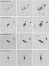 |
Fig. A.1. Examples of COCO mock images COCO-287449-153, COCO-381188-153, COCO410049-153, and COCO-98767-153 at different surface brightness limits. From left to right 29, 30, and 31 mag arcsec−2. The streams appear clearer as the depth of the image increases from left to right. All images are 10 × 10 arcmin. |
 |
Fig. A.2. Examples of TNG50 mock images TNG50-394621, TNG50-440407, TNG50-469487, and TNG50-472548 at different surface brightness limits. From left to right 29, 30, and 31 mag arcsec−2. The streams appear clearer as the depth of the image increases from left to right. All images are 10 × 10 arcmin. |
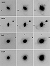 |
Fig. A.3. Examples of AURIGA mock images, Au4, Au14, Au21, and Au29 at different surface brightness limits. From left to right 29, 30, and 31 mag arcsec−2. The streams appear clearer as the depth of the image increases from left to right. All images are 10 × 10 arcmin. |
All Tables
Percentages of the principal stream morphologies in observation and simulations.
All Figures
|
Fig. 1. Examples of stellar stream images from SSLS (Martínez-Delgado 2024). The cutout angular sizes vary between 3 × 3 and 10 × 10 arcmin. The images include characteristic examples of morphological types, such as great circle (NGC 1121, UGC 8717, and 2MASXJ01463936+3206305) umbrella/shell (NGC 922 and NGC 681), and great plume (ESO 199-012), as well as those of more complex, composite morphological types (IC 169 and NGC 1097). |
| In the text | |
|
Fig. 2. Stellar mass versus B-band absolute magnitude from the Spitzer S4G catalogue. The red line represents the empirical correlation in Equation (1). |
| In the text | |
|
Fig. 3. Histogram of log10M⋆ for the observed DES sample of 689 galaxies (grey) and simulated galaxy samples from COCO (108 host galaxies, in blue) TNG50 (60 host galaxies, in red), and Auriga (30 host galaxies, in green). The black vertical line shows the average of the DES sample (log10M⋆/M⊙ = 10.00) and the dark grey vertical lines the ±1σ range around that average, [9.62, 10.38]. The light grey vertical line shows the average of the DES sample +2σ = 10.76. The maximum value of each histogram has been re-scaled to 1 for this comparison. |
| In the text | |
|
Fig. 4. Histogram of the log10 halo mass. Colours correspond to simulation sets, as shown in the legend and Figure 3. The maximum value of each histogram was re-scaled to 1 for this comparison. |
| In the text | |
|
Fig. 5. Stellar mass versus halo mass for the selected sample of galaxies in the COCO, TNG50, and Auriga simulations compared with the empirical correlation by Moster et al. (2018) ±2σ. The horizontal lines indicate the DES galaxy sample stellar mass distribution: mean value (dotted line); mean value −1σ (lower dashed line) and mean value +2σ (upper dashed line). The yellow star represents the MW. |
| In the text | |
|
Fig. 6. Example of a surface brightness map produced with pNbody. The black contours mark the isophotes of surface brightness, starting with 20 mag arcsec−2 in the centre of the host galaxy and separated by increments of 1 mag arcsec−2. |
| In the text | |
|
Fig. 7. Comparison of smoothing methods. The top panels show the surface brightness map of three different halos generated with a smoothing length up to the 16th neighbour multiplied by the factor 0.6. The bottom panels show the surface brightness maps of the same halos but applying a factor of 0.3 to the smoothing length to the 16th neighbour. |
| In the text | |
|
Fig. 8. Comparison of smoothing methods. Images generated from the surface brightness maps, by transforming the surface brightness to counts, and adding background noise to emulate a surface brightness limit of 29 mag arcsec−2. The left and centre images correspond to a smoothing length equal to the distances to the 16th nearest neighbour multiplied by a factor of 0.3 (left) and a factor of 0.6 (centre). The right panel shows the image produced with a different smoothing length, considering the distance to the fifth neighbour. |
| In the text | |
|
Fig. 9. Comparison of mock images with simulated and real DES sky background: examples of a TNG50 (left) and a COCO (right) simulated galaxy with stream stacked with a real DES sky background (panels B), and with artificial flat background (panels A) both having the same surface brightness limit of 28.65 [mag arcsec−2]. |
| In the text | |
|
Fig. 10. Stellar stream detection rate, i.e. percentage of galaxies for which at least one stream could be detected as a function of the image surface brightness limit. Continuous lines represent the results for the TNG50 (red), COCO (blue) and AURIGA (green) simulations, with error bars showing the Poisson confidence interval. The plot also shows the results of observational stream surveys from the literature, discussed in Section 7.1. (1) The calculation of the SB limit follows a different method than the one applied in this work. (2) The detection rate has been derived for all LSB features, including streams. For the DES sample (black square symbol), the x and y dimensions of the symbol indicate the dispersion in surface brightness limit of the DES sample and the dispersion in the detection rate according to a binomial distribution, respectively, see Miró-Carretero et al. (2024). |
| In the text | |
|
Fig. 11. Plot shows the log10M⋆/M⊙ distribution of the COCO halos vs the surface brightness limit at which their streams are detected. |
| In the text | |
|
Fig. 12. Stellar streams detection rate as a function of the image surface brightness limit for the TNG50 simulation. The percentage of the streams detected by visual inspection is plotted versus the surface brightness limit at which such detection was possible. The solid line corresponds to a stellar mass range of log10M⋆/M⊙ = 10.48 and log10M⋆/M⊙ = 10.76, while the dashed line corresponds to an extended mass range up to log10M⋆/M⊙ = 10.9. |
| In the text | |
|
Fig. 13. Example of the impact of the line-of-sight on morphology classification. Left: Two views of Auriga halo 14 at a surface brightness limit of 31 mag arcsec−2 from different line of sight. Right: Same views for Auriga halo 29 at a surface brightness limit of 31 mag arcsec−2. |
| In the text | |
|
Fig. 14. Histogram of the distribution of average surface brightness measured on the stream for the g (top) r (centre) and z (bottom) bands. |
| In the text | |
|
Fig. 15. Histogram of the distribution of average (g − r)0 colour measured on the stream. |
| In the text | |
|
Fig. 16. Histogram of the distribution of average distance of the streams to the centre of the host galaxy. |
| In the text | |
|
Fig. A.1. Examples of COCO mock images COCO-287449-153, COCO-381188-153, COCO410049-153, and COCO-98767-153 at different surface brightness limits. From left to right 29, 30, and 31 mag arcsec−2. The streams appear clearer as the depth of the image increases from left to right. All images are 10 × 10 arcmin. |
| In the text | |
|
Fig. A.2. Examples of TNG50 mock images TNG50-394621, TNG50-440407, TNG50-469487, and TNG50-472548 at different surface brightness limits. From left to right 29, 30, and 31 mag arcsec−2. The streams appear clearer as the depth of the image increases from left to right. All images are 10 × 10 arcmin. |
| In the text | |
|
Fig. A.3. Examples of AURIGA mock images, Au4, Au14, Au21, and Au29 at different surface brightness limits. From left to right 29, 30, and 31 mag arcsec−2. The streams appear clearer as the depth of the image increases from left to right. All images are 10 × 10 arcmin. |
| In the text | |
Current usage metrics show cumulative count of Article Views (full-text article views including HTML views, PDF and ePub downloads, according to the available data) and Abstracts Views on Vision4Press platform.
Data correspond to usage on the plateform after 2015. The current usage metrics is available 48-96 hours after online publication and is updated daily on week days.
Initial download of the metrics may take a while.