| Issue |
A&A
Volume 700, August 2025
|
|
|---|---|---|
| Article Number | A237 | |
| Number of page(s) | 34 | |
| Section | Extragalactic astronomy | |
| DOI | https://doi.org/10.1051/0004-6361/202452891 | |
| Published online | 26 August 2025 | |
The GECKOS survey: Identifying kinematic sub-structures in edge-on galaxies
1
European Southern Observatory, Karl-Schwarzschild-Straße 2, Garching 85748, Germany
2
ARC Centre of Excellence for All Sky Astrophysics in Three Dimensions (ASTRO-3D), Australia
3
School of Physics, University of New South Wales, NSW 2052, Australia
4
Centre for Extragalactic Astronomy, Department of Physics, Durham University, South Road, Durham DH1 3LE, UK
5
National Research Council of Canada, Herzberg Astronomy and Astrophysics Research Centre, 5071 W. Saanich Rd., Victoria, BC V9E 2E7, Canada
6
Centre for Astrophysics and Supercomputing, Swinburne University of Technology, PO Box 218 Hawthorn, VIC 3122, Australia
7
Astrophysics Research Institute, Liverpool John Moores University, 146 Brownlow Hill, Liverpool L3 5RF, UK
8
Sub-department of Astrophysics, Department of Physics, University of Oxford, Denys Wilkinson Building, Keble Road, Oxford OX1 3RH, UK
9
Max-Planck-Institut für Extraterrestrische Physik, Gießenbachstraße 1, 85748 Garching, Germany
10
International Centre for Radio Astronomy Research (ICRAR), The University of Western Australia, M468, 35 Stirling Highway, Crawley, WA 6009, Australia
11
Research School of Astronomy and Astrophysics, Australian National University, Cotter Road, Weston Creek, ACT 2611, Australia
12
Sydney Institute for Astronomy, School of Physics, A28, The University of Sydney, NSW 2006, Australia
13
Department of Astrophysics, University of Vienna, Türkenschanzstraße 17, 1180 Vienna, Austria
14
Observatoire de Paris, LERMA, CNRS, PSL University, Sorbonne University, 75014 Paris, France
15
Collège de France, 11 Pl. Marcelin Berthelot, 75231 Paris, France
16
Cardiff Hub for Astrophysics Research & Technology, School of Physics & Astronomy, Cardiff University, Queens Buildings, Cardiff CF24 3AA, UK
17
Instituto de Astrofísica de Canarias, Calle Vía Láctea s/n, E-38205 La Laguna, Tenerife, Spain
18
Departamento de Astrofísica, Universidad de La Laguna, Av. del Astrofísico Francisco Sánchez s/n, E-38206 La Laguna, Tenerife, Spain
19
Institute for Computational Cosmology, Department of Physics, Durham University, South Road, Durham DH1 3LE, UK
20
Homer L. Dodge Department of Physics & Astronomy, University of Oklahoma, 440 W. Brooks St., Norman, OK 73019, USA
21
Research Centre for Astronomy, Astrophysics, and Astrophotonics, Department of Physics and Astronomy, Macquarie University, NSW 2109, Australia
22
European Southern Observatory, Alonso de Córdova 3107, Vitacura, Región Metropolitana, Chile
23
Universidade Cidade de São Paulo/Universidade Cruzeiro do Sul, Rua Galvão Bueno 868, São Paulo-SP 01506-000, Brazil
24
Universitäts-Sternwarte, Fakultät für Physik, Ludwig-Maximilians-Universität München, Scheinerstr. 1, 81679 München, Germany
25
Department of Physics and Astronomy, University of Utah, Salt Lake City, UT 84112, USA
⋆ Corresponding authors: This email address is being protected from spambots. You need JavaScript enabled to view it.
Received:
5
November
2024
Accepted:
12
June
2025
Abstract
The vertical evolution of galactic discs is governed by the sub-structures within them. Several of these features, including bulges and kinematically distinct discs, are best studied in edge-on galaxies, as the viewing angle allows the easier separation of component light. For this work, we examined the diversity of kinematic sub-structure present in the first 12 galaxies observed from the GECKOS survey, a VLT/MUSE large programme providing a systematic study of 36 edge-on Milky Way-mass disc galaxies. Employing the NGIST analysis pipeline, we derived the mean luminosity-weighted line-of-sight stellar velocity (V⋆), velocity dispersion (σ⋆), skew (h3), and kurtosis (h4) for the sample, and examined 2D maps and 1D line profiles. Common clear kinematic signatures were observed: all galaxies display h3 – V⋆ sign mismatches in the outer disc regions consistent with a (quasi-)axisymmetric, rotating disc of stars. After scrutinising visual morphologies, we found that the majority of this sample (8/12) possess boxy-peanut bulges and host the corresponding kinematic structure predicted for stellar bars viewed in projection. Inferences were made on the bar viewing angle with respect to the line of sight from the strength of these kinematic indicators; we found one galaxy whose bar is close to side-on with respect to the observer, and two that are close to end-on. Four galaxies exhibit strong evidence for the presence of nuclear discs, including central h3–V⋆ profile anti-correlations, croissant-shaped central depressions in σ⋆ maps, strong gradients in h3, and positive h4 plateaus over the expected nuclear disc extent. The strength of the h3 feature corresponds to the size of the nuclear disc, measured from the h3 turnover radius, taking into account geometric effects. We can explain the features within the kinematic maps of the four unbarred galaxies via disc structure(s) alone. We do not find any need to invoke the existence of dispersion-dominated bulges in any of the sample galaxies. Obtaining the specialised data products for this paper and the broader GECKOS survey required significant development of existing integral field spectroscopic (IFS) analysis tools. Therefore, we also present the NGIST pipeline: a modern, sophisticated, and easy-to-use pipeline for the analysis of galaxy IFS data, and the key tool employed by the GECKOS survey for producing value-added data products. We conclude that the variety of kinematic sub-structures seen in GECKOS galaxies requires a contemporary view of galaxy morphology, expanding on the traditional view of galaxy structure, and uniting the kinematic complexity observed in the Milky Way with the extragalactic.
Key words: galaxies: bulges / galaxies: evolution / galaxies: general / galaxies: kinematics and dynamics / galaxies: structure
© The Authors 2025
 Open Access article, published by EDP Sciences, under the terms of the Creative Commons Attribution License (https://creativecommons.org/licenses/by/4.0), which permits unrestricted use, distribution, and reproduction in any medium, provided the original work is properly cited.
This article is published in open access under the Subscribe to Open model. This email address is being protected from spambots. You need JavaScript enabled to view it. to support open access publication.
1. Introduction
Most galaxies are multi-component systems that consist of multiple photometrically, chemically, and kinematically distinct stellar structures. In the local Universe, the majority of Milky Way-mass galaxies comprise a rotationally supported disc (e.g. Guo et al. 2020), a bulge1 (e.g. Gadotti 2009), a stellar bar (e.g. Erwin 2018), and a diffuse stellar halo (e.g. Helmi 2020).
The Milky Way itself is largely considered to be a typical disc galaxy (e.g. Bland-Hawthorn & Gerhard 2016). In addition to the structural components listed above, the Milky Way disc may be separated into two chemically distinct discs, whose stellar populations can be divided into two groups: young, metal-rich, and [α/Fe]-poor; and old, metal-poor, and [α/Fe]-rich (e.g. Gilmore & Reid 1983; Haywood et al. 2013; Hayden et al. 2015). Observations of external galaxies have hinted at similar chemical structures (e.g. Pinna et al. 2019a,b; Scott et al. 2021). The kinematic thick disc of the Milky Way has also been found to host stars with a larger velocity dispersion and slower net rotation than stars in the thin disc (e.g. Chiba & Beers 2000; Soubiran et al. 2003; Girard et al. 2006). Similar vertical dispersion gradients are also seen in external galaxies (e.g. Yoachim & Dalcanton 2008; Comerón et al. 2019; Pinna et al. 2019a,b; Kasparova et al. 2020; Martig et al. 2021; Bhattacharya et al. 2023). Lastly, the Milky Way also hosts a bar and a boxy-peanut (BP) bulge (e.g. Kent et al. 1991; Wegg & Gerhard 2013; Ness & Lang 2016). This means that the integrated kinematic measurements along a line of sight in an extragalactic Milky Way-like galaxy will include contributions from at least four different kinematic sub-structures near the centre.
The diversity of the galactic kinematic sub-structure is most conspicuous in the central regions, where many structures may contribute to the overall surface brightness distribution. Each sub-structure hosts stars on specific orbits, though the diversity of central structure (including the relative contributions of various stellar orbital families) is not well quantified and lacks comprehensive kinematic descriptors to categorise the central structure, despite many efforts (e.g. Fabricius et al. 2012; Méndez-Abreu et al. 2014). In fact, it seems that the more depth with which one studies galactic sub-structures, the more complicated they become (e.g. Gadotti et al. 2020).
Edge-on galaxies represent a unique opportunity to study galactic central components, as the light that bulges out of the disc is readily observable for these geometries. One such central structure to which much work has been devoted is the BP bulge (e.g. Burbidge & Burbidge 1959; Lütticke et al. 2000), widely believed to be the out-of-plane projection of a buckled stellar bar (e.g. de Souza & Dos Anjos 1987; Kuijken & Merrifield 1995; Bureau & Freeman 1999). Present in ∼80% of Milky Way-mass galaxies (Erwin & Debattista 2017), this structure is a natural consequence of disc galaxy evolution (e.g. Combes & Sanders 1981; Debattista et al. 2006; Valluri et al. 2016; Fragkoudi et al. 2017; Parul et al. 2020; Tahmasebzadeh et al. 2024). Detecting the presence of a BP bulge and bar can be difficult from imaging alone, as these structures leave distinct photometric imprints for only a limited range of bar viewing angles. Complicating matters, they can visually resemble a ellipsoidal ‘classical’ bulge in projection when viewed end-on (e.g. Combes et al. 1990; Laurikainen & Salo 2017). For this reason, the addition of kinematic information can aid in identifying BP bulges and bars within their host galaxies.
Significant progress in quantifying the motions of stars within BP bulges has been made, both in- and off-plane. Several studies have applied stellar kinematic indicators to classify the behaviour of the stars (e.g. Chung & Bureau 2004; Bureau & Athanassoula 2005; Méndez-Abreu et al. 2008, 2014), and dynamically, the bar orbits are well-understood and modelled. Barred galaxies contain stars on more elongated orbits, chiefly the x1 orbits coincident with the canonical bar shape, and the x2 orbits, which are smaller, generally more circular, and oriented perpendicular to the x1 orbits (e.g. Athanassoula 1992; Sellwood & Wilkinson 1993). The angle at which the bar is viewed by the observer (i.e. more side-on or more end-on) determines (i) the relative contribution of each bar orbit family to a given line-of-sight velocity distribution (LOSVD) and (ii) the shape of the LOSVD of that orbit (as bar orbits are not axisymmetric); hence, the bar viewing angle has a measurable effect on the stellar kinematics observed.
Chung & Bureau (2004) and Bureau & Athanassoula (2005) investigated the kinematics of BP bulge galaxies and compiled a set of kinematic criteria from long-slit observations that described the various structures present in the mid-plane. They describe rotation curve ‘humps’, and velocity dispersion peaks and plateaus. They also see a complex relation between the mean velocity (V⋆) and the skewness of the LOSVD (h3), which anti-correlate, correlate, and anti-correlate again in the nuclear disc, bar, and outer disc regions, respectively. Taken together, these models and observations provide a solid foundation to begin investigating the kinematic sub-structure behaviour, although only in one dimension (i.e. radially along the mid-plane).
The advent of large-scale integral field spectroscopic (IFS) observations, including highly spatially resolved observations, has allowed studies off the plane of galactic discs and prompted observations of kinematic structures in the form of 2D moment maps (e.g. de Zeeuw et al. 2002; Guérou et al. 2016; Pinna et al. 2019a; Poci et al. 2019; Martig et al. 2021). Motivated by the influx of such data, studies such as Iannuzzi & Athanassoula (2015) and Li et al. (2018) have provided a set of 2D kinematic predictors of various central structures, including BP and classical bulges. The off-plane structure of the kinematic high-order moments is coherent, and 1D long-slit data insufficient to fully describe the kinematic trends seen in BP bulge galaxies. The more complex AURIGA cosmological zoom-in simulations (Grand et al. 2017) confirm that off-plane kinematic structure is a regular feature in disc galaxies (Pinna et al. 2024), and that BP bulges contribute to distinct kinematic signatures in the inner regions of galaxies (Fragkoudi et al. 2020).
Much can also be learnt about stellar kinematic distributions from simpler analytic galactic models. Wang et al. (2024) generated mock IFS data cubes of the Milky Way by forward-modelling the chemodynamical model of Sharma et al. (2021). Based on star particles distributed in a simple disc structure (i.e. no bulge, halo, or nuclear disc structure), outputs were provided in the form of spatially binned 2D maps of stellar velocity moments, allowing a direct comparison to observations. In particular, once analysed by industry-standard spectral fitting packages, output stellar velocity dispersion maps displayed high dispersion values in the central region and up to several kiloparsecs off the plane, much higher than the input from the mock IFS cube. Importantly, this dispersion peak was caused only by the disc structure; there was no central spheroid included in these models.
Some galactic features are difficult to model. The small scales of some central galactic features such as nuclear discs (Gadotti et al. 2020) have precluded them from being resolved in cosmological or even zoom-in simulations. The numerical heating of stellar particles also wreaks havoc on the size and shape of small thin discs, even at high resolutions (e.g. Ludlow et al. 2019; Galán-de Anta et al. 2023). Furthermore, most mock observations from simulations tend not to include typical observational features such as dust lanes, although some advances have been made in this area (e.g. Barrientos Acevedo et al. 2023). Given the prevalence and obvious complexity of galactic kinematic sub-structures coupled with both simulation predictions and limitations, a census of kinematic sub-structures in a representative sample of Milky Way-mass galaxies will allow us to make progress towards a better interpretation and framework of all central disc structures.
In this paper we categorise the diversity of kinematic sub-structures in the first 12 galaxies observed as part of the GECKOS2 survey. Our aim is to define a range of kinematic sub-structures and link them to the assembly and evolutionary history of the host galaxies. In Section 2 we describe the GECKOS survey (including data reduction and analysis) and ancillary data. In Section 3 we identify BP bulges from imaging and present 1D and 2D stellar kinematics. In Section 4 we interpret the results within a framework of galactic central structure assembly. We also introduce the NGIST 3 package in Appendix A; it is a modern freely available IFS data analysis package, flexible enough to analyse any galaxy IFS data. Throughout this paper, we use ΛCDM cosmology, with Ωm = 0.30, ΩΛ = 0.70, and H0 = 70 km s−1 Mpc−1, and a Chabrier (2003) initial mass function.
2. Data
Our sample consists of the first 12 galaxies from the GECKOS survey, an ESO/VLT large programme awarded 317 hours on MUSE (van de Sande et al. 2024). In Section 2.1-2.3 we summarise the sample selection, observing strategy, and data reduction respectively, but a full description will be presented in van de Sande et al. (in prep.). We also introduce the updated data analysis pipeline package NGIST in Section 2.4 and Appendix A.
2.1. GECKOS sample
GECKOS aims to investigate the relative importance of the internal and external physical processes that drive the evolution of disc galaxies. The GECKOS MUSE survey consists of 36 edge-on disc galaxies, covering out to a surface brightness of  , similar to that at the Sun’s position in the Galactic disc when viewed face-on (Melchior et al. 2007). Targets were selected within a distance range of 10 < D [Mpc]< 70, 25 of which were sourced from the S4G survey (Sheth et al. 2010) and the remaining 11 from HyperLeda (Makarov et al. 2014). Seven of these galaxies that meet our sample selection criteria possess MUSE archival observations.
Galaxies with a stellar mass within ±0.3 dex of the Milky Way ( ; Bland-Hawthorn & Gerhard 2016) that are edge-on (or highly inclined) are targeted. Furthermore, GECKOS aims to include a diversity of morpho-kinematic and star formation properties by selecting galaxies within a 2 dex range of mid-IR-derived star formation rates (SFRs; Cutri et al. 2013; Leroy et al. 2021). The GECKOS targets are evenly divided into three bins of SFR, comprising a sub-main sequence, a main sequence, and a super-main sequence sample. This spread in SFR not only maximises the variety of possible assembly histories, but also increases the probability of detecting outflows, present in ∼30 − 50% of main sequence galaxies (Stuber et al. 2021) and ubiquitous in starbursts (e.g. Veilleux et al. 2020).
Galaxies with clear signs of ongoing or recent mergers are avoided, as are those near the centre of clusters where external gas-removal processes may strongly impact disc evolution (e.g. Cortese et al. 2021). The final GECKOS sample contains BP bulges, non-BP bulges, and some galaxies with no visible bulge, with the hope being that given the diversity in observables, as wide a range in assembly histories as possible is covered.
For this paper we used all galaxies whose observations were completed by December 2023, for either the entire galaxy or the central pointing. This sub-set of galaxies forms the core of the GECKOS first internal data release (iDR1) and includes fully reduced and mosaicked data cubes for the galaxies ESO 484-036, NGC 5775, ESO 079-003, UGC 00903, ESO 120-016, NGC 3279, NGC 0360, PGC 044931, IC 1711, and NGC 3957, and the central pointing only of NGC 0522 and IC 5244. While not a statistical nor representative sample of the local Universe, this sub-sample contains galaxies from all three bins of star formation rate, and is hence a representative sample of GECKOS galaxies.
2.2. GECKOS MUSE observing strategy
GECKOS galaxies are observed using VLT/MUSE (Bacon et al. 2010) in wide-field mode (field of view 1′ × 1′,  pixel sampling), and the nominal wavelength coverage of 4800–9300 Å with 1.25 Å pixel−1 wavelength sampling (R ∼ 3000). The GECKOS tiling strategy is based on the science requirement to measure the stellar kinematics and stellar populations out to the 23.5 V mag arcsec−2 isophote.
Depending on the distance to each galaxy, one MUSE pointing is required for the most distant galaxies, and up to six radially tiled pointings for the nearest objects. For the super-main sequence sample, the MUSE coverage extends to a height of 10 kpc, based on the extent of the outflow in M82 (Shopbell & Bland-Hawthorn 1998). For the six most highly star-forming galaxies, we therefore add a pointing off the plane of the disc near the centre.
All galaxies are observed in natural seeing conditions. However, to ensure a spatial resolution of < 200 pc as set by the science requirements, depending on the distance to the target, we requested the observations to be carried out in the turbulence category < 30%–< 85%, or a seeing threshold of 0 7–1
7–1 3 (Martinez et al. 2010). Exposure times were calculated using the ESO MUSE exposure time calculator based on a S/N requirement of S/N > 40 Å−1 for a spatial bin with a maximum size of 200 pc.
Observations commenced in October 2022 and were carried out in service mode, split into one-hour observation blocks (OBs). Within each OB, four ∼9 − 10 min object (O) and two ∼2 − 3 min sky observations (S) were executed in an OSOOSO sequence. Within each one-hour OB, four 90 degree rotations combined with small offset dithers were used to optimise data homogeneity in the final cube. Between pointings, a 3″ overlap was adopted to create a smooth and continuous final mosaicked data cube.
2.3. Data reduction
The dedicated PYTHON package PYMUSEPIPE v2.23.4 4 was utilised to calibrate the science exposures and create mosaicked data cubes. PYMUSEPIPE is a nearly fully automated pipeline, described in detail in Emsellem et al. (2022). It serves as a data organiser and wrapper for the sequential execution of the ESO Recipe Execution Tool (ESOREX; ESO Cpl Development Team 2015) recipes, and also provides additional utilities for improved alignment, flux and sky calibration, and mosaicking. PYMUSEPIPE is built around the MUSE Data Reduction Pipeline (DRP) that was developed to remove instrumental signatures (Weilbacher et al. 2020)5. A full description of the GECKOS data reduction workflow will be presented in van de Sande et al. (in prep.), and we note that a similar setup was used in Watts et al. (2024).
Three-colour g′ri images reconstructed from the MUSE cubes of the 12 galaxies used in this paper are shown in Figure 1. We note here that while the MUSE nominal wavelength range of ∼4800–9300 Å covers the SDSS r and i bands well, the g band is truncated, and so we refer to it as g′. The reconstructed g′ band image follows the SDSS g-band filter response curve for ∼4800–5500 Å.
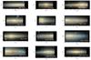 |
Fig. 1. g′ri colour images of the sample galaxies reconstructed from the MUSE data cubes of the first 12 galaxies observed as part of the GECKOS survey. In each case, the mosaicked cube has been rotated and aligned such that the photometric major axis is horizontal, and if the dust lane is offset from it, it is always on the lower side of the image. For galaxies not exactly edge-on this means that we look at them from above (i.e. the lower half is the near half) if the dust lane is assumed to be in the mid-plane of the galaxy. The GECKOS pointing strategy was such that the entire (visible) bulge was always included within the MUSE field of view, and at least one side of the galactic disc. Here we show only regions where the signal-to-noise ratio is greater than 2.5; the MUSE field of view often extends further vertically. |
2.4. Data analysis
There exist many pipelines for the analysis of IFS data, several of which wrap existing well-established spectral fitting routines, for example, the data analysis pipelines of MaNGA (Westfall et al. 2019) and PHANGS (Emsellem et al. 2022), PIPE3D (Sánchez et al. 2016) and the GIST pipeline (Bittner et al. 2019). The future of extragalactic, spatially resolved spectroscopy will involve pushing current instrumentation to its limits, requiring highly customisable analysis software packages. The GECKOS survey alone necessitates the development of techniques to deal with low S/N, and highly sky-dominated regions to extract science from the galactic outer disc regions. Additionally, large co-added mosaics of several pointings of nearby galaxies are becoming a common technique to resolve the small-scale physics driving galaxy evolution. Such mosaics are large, and computationally expensive to run through existing, non-optimised software. Here, we present NGIST, an upgraded version of the GIST pipeline, with added features, improved usability, and retained functionality and core principles. Described more fully in Appendix A, NGIST is publicly available, documented, and maintained via a GitHub repository.
NGIST is flexible, and allows user specification of over 40 different variables via a compact and human-readable configuration file. A full description of all input parameters used for GECKOS iDR1 for each NGIST module will appear in van de Sande et al. (in prep.) and the NGIST documentation6. Here, we describe the data products produced and employed in this work.
For this work, we employ the NGIST version 7.2.1 to output 2D maps of stellar kinematics Voronoi binned to S/N = 100 pixel−1 (or 80 Å−1, calculated over 4800–7000 Å). We chose this wavelength range so that the S/N estimate includes a minimal number of sky lines. We chose this binning S/N to ensure the highest-quality kinematic maps possible, whilst noting that the science goals mostly concern the central regions of the galaxies for this work, where S/N is typically very high. Spaxels with a S/N < 5 were masked along with bright stars and any other contaminating foreground objects. We tested the effects on the derived stellar kinematics from the wavelength range employed. We present the results in Appendix C, and determine that for our science goal of understanding the kinematics of structures at the centres of galaxies, whilst still recovering h3 and h4 in the outskirts of low-dispersion discs, a wavelength range of 4800–8900 Å yielded the best results compared to small ranges centered on individual features such as Hβ and Mg b in the blue and the Calcium II triplet (CaT) in the red. All spectroscopic analyses are run over the wavelength range 4800–8900 Å, and a Milky Way foreground dust extinction was calculated and corrected for, using the Cardelli et al. (1989) dust extinction model.
The NGIST stellar kinematics (KIN) module employs the PYTHON implementation of the penalised Pixel Fitting (PPXF) routine of Cappellari & Emsellem (2004) and Cappellari (2017) and the X-shooter stellar library DR3 (Verro et al. 2022). We chose the X-shooter library for its extended wavelength coverage and excellent spectral resolution about the CaT, and following the recommendations of previous works that stars are generally preferred over SSPs for stellar kinematic determinations (e.g. van de Sande et al. 2017; Belfiore et al. 2019). Motivated by previous IFS works including SAURON (Emsellem et al. 2004), ATLAS3D (Cappellari et al. 2011), SAMI (van de Sande et al. 2017), MaNGA (Belfiore et al. 2019; Westfall et al. 2019), and PHANGS (Emsellem et al. 2022), to improve the quality of the derived kinematics, we fit a 23rd order additive Legendre polynomial to provide a closer match between data and the spectral templates. This polynomial order was guided by the detailed analysis of the effect of polynomial order as a function of wavelength range by van de Sande et al. (2017). We additionally fit a first-order multiplicative polynomial, to mitigate any small variation in continuum shape from imperfect sky subtraction and dust attenuation. We mask spectral regions affected by sky emission and nebular gas emission lines. Initial guesses for velocities were taken from the NASA Extragalactic Database, and an initial guess for the stellar velocity dispersion of 100 km s−1. Example spectral fits can be seen in Figure A.4.
We use a PPXF penalising bias optimised for our specific science case. The default penalisation is too high, in particular in the outer discs where the velocity dispersion is close to, or below the instrumental resolution. In those regions, the default or auto bias resulted in the high-order moments being penalised to zero, whereas a run without any penalising bias showed a significant detection of h3 and h4.
Following the recommendations outlined in the PPXF code documentation, we determined the optimised bias value by performing a large ensemble of Monte Carlo simulations, testing how well the LOSVD parameters are recovered as a function of velocity dispersion. The ideal bias is defined as one that reduces the scatter in the velocity dispersion, h3 and h4, without creating a systematic offset in the velocity and velocity dispersion when the dispersion is larger than the spectrum’s velocity scale (41 km s−1). In the tests, we used a MILES SSP with an age of 5.01 Gyr, [M/H] = 0.0, and a wavelength range of 4800–7000 Å.
Based on the examples in Emsellem et al. (2004), Cappellari et al. (2011), and van de Sande et al. (2017), we derived a simple analytic expression for the ideal penalising bias for MUSE spectra as a function of S/N, implemented by invoking the muse_snr_prefit option for the BIAS keyword in NGIST. We find
 (1)
(1)
To account for changes in the wavelength range and a number of masked spectral pixels, we then adopt a function similar to the PPXF auto bias:
 (2)
(2)
Here Nλpixels is the number of unmasked spectral pixels used in the PPXF fit.
For an S/N = 100 and wavelength range of 4800–5500 Å, 4800–7000 Å, and 4800–8900 Å, typical values for the penalising bias are 0.27, 0.18, and 0.14, respectively. For our study, we use the S/N of each individual Voronoi bin to calculate the optimal bias.
2.5. Imaging
For comparison to kinematic indicators, we examined the visual morphologies of the galaxies. r-band The Dark Energy Camera Legacy Survey (DECaLS) images (Dey et al. 2019) are available for the whole sample, which were downloaded as 10-arcmin cutouts. Mid-IR imaging suffers less from dust obscuration, and can therefore help identify structures that would otherwise have been hidden by dust. Spitzer imaging is available for NGC 3957, NGC 0522, IC 1711, NGC 0360, UGC 00903, NGC 3279, and NGC 5775, and cutouts of 3.6 μm imaging were obtained for these galaxies from the NASA IPAC Infrared Science Archive, shown in Appendix D.
3. Results
3.1. Off-plane structure from unsharp masked imaging
We first wish to classify the visual morphology of the off-plane structures in the GECKOS galaxies. To do so, we examine unsharp-masked DECaLS DR9 r-band images of each galaxy in the sample and 3.6−μm Spitzer imaging where available. To supplement our imaging data, we also refer to historical morphological classifications from the literature.
Unsharp masking is a common technique whereby a smoothed version of an image is divided by the unsmoothed version to highlight ‘sharp’ high-spatial-frequency features. It has been shown to work well for identifying X-shaped BP bulge features (e.g. Aronica et al. 2003; Bureau et al. 2006; Laurikainen & Salo 2017). We chose DECaLS imaging for this task, as it has good spatial resolution and an average full width at half maximum of 1″.2 in the r band (Dey et al. 2019). In addition, this imaging is available for the entire GECKOS iDR1 sample. We note that the three-colour images derived from the MUSE cubes themselves could also be suitable for this purpose, though given that the whole galaxy is not included in the MUSE field of view, it can be a little more difficult to elucide central structures. We first smooth a DECaLS r-band cutout image of each galaxy with a 2D circular Gaussian kernel with σ = 7 − 20 pixels depending on galaxy distance (corresponding to ∼2 − 5″), and then divide the original image by this smoothed image.
The results of the unsharp masking are shown in Figure 2. Immediately, we identify two obvious X-shaped bulges from the DECaLS imaging: PGC 044931 and NGC 0522. In addition, faint peanut-shaped structure is seen in IC 5244, IC 1711, ESO 079-003, ESO 484-036, and possibly ESO 120-016. NGC 3279 and UGC 00903 do not display any BP bulge structure, and while spiral arms are visible in NGC 0360 and NGC 5775, no vertically extended bulge features are seen in these galaxies, either.
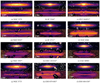 |
Fig. 2. r-band DECaLS image (top) scaled with an inverse hyperbolic sine (arcsinh) scaling with surface brightness contours overlaid in white (units of r-band magnitude arcsec−2), and unsharp masked image created with a Gaussian smoothing kernel of width σ = 7 − 20 pixels (bottom). Galaxy names marked with a ⋆ are considered to host a boxy-peanut central structure in this work. The orientation of galaxies here, and throughout, is the same as in Fig. 1. |
IR imaging can also help to reveal BP bulge structures as it suffers less from dust obscuration, and Spitzer 3.6 μm imaging is shown where available in Figure D.1. We also perform unsharp masking on the 3.6 μm imaging as a comparison. We note that a faint boxy or peanut shape is visible in NGC 3957, NGC 0522, and IC 1711, and clear spiral arms for NGC 0360 and NGC 5775.
From the combined DECaLS and Spitzer images (where available), we reach the consensus that NGC 3957, PGC 044931, NGC 0522, IC 1711, IC 5244, ESO 079-003, and ESO 484–036 contain BP bulge structures. For ESO 120-016, we find tentative evidence for a boxy shape.
3.2. Visual morphologies from the literature
There have been several previous surveys that classified central structure in large samples of galaxies from imaging of varying spatial resolution, including Lütticke et al. (2000) and Buta et al. (2015). The results of literature classifications for the galaxies in this work are shown in Table 1, along with the classifications from unsharp masking described above. Neither ESO 484-036 nor PGC 044931 were classified by either of these works, though PGC 044931 has been studied extensively and classified as boxy/peanut by works such as Bureau & Freeman (1999) and Chung & Bureau (2004). The classification of NGC 3957 by Bureau & Freeman (1999) differs from Lütticke et al. (2000), where the former classifies it as an ellipsoidal bulge, while the latter calls it boxy. In this current work, we see a clear X-shape in the Spitzer imaging, confirming the unsharp masking results of Bureau et al. (2006). Lütticke et al. (2000) also classify NGC 0360 as ‘close to box-shaped’, while we see no evidence of this in the DECaLS or Spitzer imaging. Indeed, central, tightly wound spiral arms are clearly visible in the 3.6 μm imaging, which may have been confused for a box shape in optical and lower-resolution imaging. Given the poor spatial resolution of DSS imaging, we take the classifications from this current work, Buta et al. (2015), and Bureau & Freeman (1999) as our primary references.
Summary of galaxy morphological classifications from the literature.
3.3. Stellar kinematic maps and radial profiles
In Figures 3 and B.1–B.11, we present the derived stellar line-of-sight luminosity-weighted mean velocity (V⋆), velocity dispersion (σ⋆), and high-order moments skew (h3) and kurtosis (h4) for the GECKOS galaxies, derived over the wavelength range 4800–8900 Å. We also tested just the Calcium II triplet (CaT) range (8450–8735 Å, similar to McDermid 2002), but found that while the redder wavelength range resulted in more spatially coherent structure in the high-order moment maps, this short wavelength range often failed to produce a cohesive h3 and h4 signal in the outer, lower dispersion regions of some of the galactic discs. For a further discussion of wavelength-dependent kinematic structures, see Appendix C. In Figures 3 and B.1–B.11 each galaxy is rotated such that the photometric major axis lies horizontal and the dust lane (if offset), is always to the lower side of the image. We note that for some galaxies, the MUSE mosaic covers only one side of the disc. The GECKOS pointing strategy was such that the entirety of the bulge was included in the MUSE pointings, however. At first glance, all galaxies appear to host regularly rotating discs. However, upon more careful examination, the diversity in structure in the kinematic maps isconsiderable.
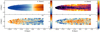 |
Fig. 3. Stellar luminosity-weighted line-of-sight velocity, V⋆ (top left), velocity dispersion, σ⋆ (top right, with r-band surface brightness contours overlaid in white), h3 (bottom left) and h4 (bottom right) maps derived with NGIST and binned to S/N = 100 for the galaxy NGC 3279, a galaxy with no obvious visual bulge structure. Galaxies are shown such that the dust lane (and photometric major axis) are oriented horizontally, and such that the dust lane (if offset) is to the lower side of the image. Holes in the maps are regions where bright stars have been masked. Flux contours are overlaid on the σ⋆ maps to highlight the dust lane effects, but not for the V⋆, h3, and h4 maps, to aid in central structure recognition. |
For a more straightforward comparison to previous literature, Figures 4 and 5 depict the 1D radial profiles extracted from the corresponding 2D maps. These profiles were extracted from slits of width 1 kpc between  , which we found to be wide enough to encompass central kinematic structure of interest, whilst minimising the contribution of dust lane regions, keeping in mind that the dust lanes are always offset to the lower side of the images for which we place the slits on. Furthermore, rather than presenting h3 directly against V⋆, we present all 1D kinematic quantities as a function of galactocentric radius. To facilitate interpretation, for 1D profiles we compare the radial gradients of V⋆ and h3, where if both gradients are positive or negative, the quantities are correlated, but if one is positive and the other is negative, the two quantities are anti-correlated. For the 2D maps, we discuss the sign of the V⋆ and h3 regions (i.e. a positive value of V⋆ and h3 have a matching sign).
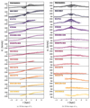 |
Fig. 4. 1D line profiles, extracted from slits of |

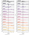 |
Fig. 5. As in Figure 4, but for the 1D line maps of h3 (left) and h4 (right). The typical median errors are h3, err = 0.016 and h4, err = 0.017. |
To aid in the recognition of kinematic structure, we have flipped the direction of the profiles of ESO 120-016, NGC 0360, NGC 0522, ESO 484-036, IC 1711, and IC 5244 such that the receding side of the resultant rotation curve is on the right for all galaxies. Below, we describe the trends seen in the 2D kinematic maps and 1D radial profiles, and in Section 4 we interpret these results in terms of galactic sub-structures.
3.3.1. Velocity maps and profiles
The top left panels of Figures 3 and B.1–B.11 display velocity (V⋆) maps, corrected for systemic velocity using a box of width 2 kpc extending perpendicular to the galaxy kinematic major axis, centred on the flux centre of the galaxy, and extending to only the side of the galaxy that is less dust affected (i.e. positive values of z in Figures 3 and B.1–B.11). We mask regions with E(B-V) > 0.4, and recalculate the median velocity within this region before subtracting it from the maps. In all cases, we see evidence of well-behaved, regularly rotating discs, with the notable exception of UGC 00903, which appears to comprise two counter-rotating stellar discs (see van de Sande et al. in prep. for further insight). In some cases, the dust lane is evident as a region lighter in colour, indicating velocity magnitude lower than its surroundings, located just below the z = 0 line. For many galaxies the V⋆ = 0 isovelocity line is not straight; rather, often warps, wedges, or other structures are visible both along the z = 0 line, and at higher latitudes. For several galaxies (e.g. PGC 044931, NGC 0522, NGC 0360, and ESO 079-003), the kinematic minor axis displays a wedge-like structure within ±0.5kpc of the z = 0 line. The co-spatial nature of young stars and dust make light-weighted stellar kinematic maps difficult to interpret in highly obscured regions, though we speculate on the commonly observed features in Section 4.1.2.
For IC 1711, NGC 3957, and PGC 044931, the most striking feature is a small, darker-coloured region within the central kiloparsec that is rotating faster than the surrounding disc, likely a kinematically decoupled discy component. For comparison to previous literature, in Figure 4a, we plot the galaxy rotation curves, extracted from slits of width 1 kpc. All galaxies host rapidly rising rotation curves, though the slope of the curve is much steeper in the central regions of PGC 044931, NGC 3957, IC 1711, and IC 5244. The characteristic ‘double-humped’ rotation curve (i.e. a rotation curve that first rises rapidly to reach a local maximum, then drops slightly to create a local minimum, and then rises again slowly up to its flat section) described by Bureau & Athanassoula (2005) is seen in these four galaxies.
3.3.2. Stellar velocity dispersion, σ⋆, maps and profiles
The top right panels of Figures 3 and B.1–B.11 show σ⋆ maps. Here, we see a great deal of variation between galaxies, and several features of note. First, we acknowledge the dark purple strips of low σ⋆ crossing most galaxies, coincident with the position of the dust lane, and highlighted by the non-symmetric nature of the flux contours overlaid in white. Given that dust blocks light from the galactic plane regions from reaching the observer, we expect to be viewing just the stars which are intrinsically exterior to the dust lanes in these regions.
In addition to the dust lanes, we also observe central regions of high-velocity dispersion, transitioning to lower dispersion at greater radii in most of the galaxies, except NGC 3279 and UGC 00903. Central σ⋆ maxima range from 70–130 km s−1, with an average of σ⋆ ∼ 90 km s−1. The increase in σ⋆ from the outskirts to the central regions, Δσ⋆, is on average ∼50 km s−1. In NGC 3957 and PGC 044931, this central high σ⋆ region is ‘croissant-shaped’, with a lower dispersion region embedded within the high σ⋆ region at the centre of the galaxy. We expect that these are not the result of dust obscuration, as neither of these galaxies is perfectly edge-on and the effect of the dust is visible below the z = 0 line. Additionally, the low σ⋆ regions are offset from the projection of the main dust lane in the 2D maps; co-located with the kinematically decoupled disc indicator seen in the V⋆ maps. For IC 5244 and IC 1711, the central region withσ⋆ > 100 km s−1 is extended and nearly circular, with dispersions exceeding 110 km s−1.
Correspondingly, the 1D σ⋆ profiles shown in Figure 4b are also quite varied. While some galaxies host gently peaked line profiles, the strong peaks of IC 1711 and IC 5244 are clear. Interestingly, a large spread in central σ⋆ is seen in the four galaxies with the steepest-rising rotation curves: IC 5244, IC 1711, NGC 3957, and PGC 044931.
3.3.3. Skew, h3, maps and profiles
The bottom left panels of Figures 3 and B.1–B.11 show the high-order Gauss-Hermite moment h3 (or skew). The colour map is such that red indicates a positive skew value (where excess low velocities are present in the LOSVD beyond that of a pure Gaussian), and blue a negative (where excess high velocities are present in the LOSVD). While there is more stochasticity between neighbouring bins than the V⋆ and σ⋆ maps, some spatially coherent features are readily visible.
We observe small, oval-shaped regions of highly positive and negative h3 at the very centre of the galaxy and only along the z = 0 line for IC 5244, IC 1711, NGC 3957, and PGC 044931. Compared to their V⋆ maps, these regions are opposite in sign. Additionally, this feature is also seen in the 1D radial profiles of Figure 5a. A strong, negative gradient in h3 as a function of galactic radius is seen in the h3 profiles of PGC 044931, NGC 3957, IC 1711, IC 5244, and UGC 00903. For these galaxies, the extrema of the h3 coincide radially with the V⋆ humps pointed out in Section 3.3.1. The two h3 extrema present close to the galaxy centre imply large gradient in the central h3 radial 1D profile between them, and since the signs of these extrema are opposite to those of V⋆, the corresponding gradient of the V⋆ radial profile is of opposite sign and therefore h3 and V⋆ anti-correlate within the radius of the h3 extrema. We expect these features to be the signature of a dynamically cold disc, and discuss them further in Section 4.2.
At larger scales, we see varying h3 behaviour along the z = 0 line compared to off the plane for a given R in several galaxies: NGC 3957, NGC 0522, PGC 044931, IC 5244, and perhaps best illustrated in ESO 079-003. We observe ∼0.5 kpc-wide strips where h3 and V⋆ are of opposite sign along the kinematic major axis of these galaxies, discussed in Section 4.1.3. These strips often extend to the radial extent of the MUSE field of view. We note that the correlations seen in 1D profiles often extend only to small scales (e.g. ∼1 kpc for IC 1711), whereas when sign-matching, additional coherent regions of sign matching and mismatching are also obvious at larger scales. For IC 1711, both above and below the z = 0 line, these opposing signs in V⋆ and h3 switch to matching signs, and we observe coherent positive (negative) regions of h3, corresponding to positive (negative) values of V⋆, extending 0–3 kpc radially, and 0.5–2 kpc off the z = 0 line of the disc. We see the largest regions of matching h3 and V⋆ sign in IC 5244, and IC 1711, but also see this feature to varying degrees in all other BP bulge galaxies, though the signal is faint in ESO 120-016 and NGC 0522. In the radial outskirts of all galaxies in this sample, we note coherent regions of h3 and V⋆ opposing signs, extending to the edges of the MUSE field of view. For galaxies with the most coherent h3 structure, moving from the central regions to the galactic outskirts, we observe the signs of h3 and V⋆ to oppose, match, and then oppose again.
We note that for PGC 044931 (Fig. B.2) and NGC 0360 (Fig. B.5) the h3 values in the very outer disc region tend to zero. There are several possible causes for this behaviour, including inappropriate penalisation of the PPXF solution in the outermost bins, most of which possess a lower S/N than the desired value. Even with a S/N-dependent PPXF bias determination, we found that outer bins were extremely susceptible to small changes in penalising bias. The h3 behaviour seen is also common when the measured velocity dispersion is well below the instrumental resolution, and also present in the work of e.g. Seidel et al. (2015) for the SAURON spectrograph, and in mock IFS datacubes by Wang et al. (2024). In the wavelength range investigated in this work, the MUSE spectral resolution is ∼40 km s−1 (e.g. Bacon et al. 2017). The measured σ⋆ of both PGC 044931 and NGC 0360 in the outskirts of their discs is ∼20 km s−1. For this work, we are interested mostly in the central regions of the galaxies, where the dispersion is higher, whereas the analysis of the kinematics in the outskirt regions will be presented in future work.
3.3.4. Kurtosis, h4, maps and profiles
In Figures 3 and B.1–B.11, we present the line-of-sight kurtosis, or h4, maps. There are fewer spatially coherent features visible in these maps, possibly the result of observational challenges related to retrieving high-order velocity moments from medium-resolution spectra (e.g. Wang et al. 2024). Nevertheless, we do notice some trends. Given their co-spatial nature, we expect that the large longitudinally extended regions of high positive h4 around the centres of some galaxies that correspond to low σ⋆ and clear deviations from symmetry in the surface brightness contours are caused by the dust lanes. In some galaxies, including PGC 044931, NGC 3957, NGC 0522, and ESO 079-003, we see regions of high positive h4 extending from the central regions of the galaxy 1–2 kpc off the z = 0 line. In PGC 044931, IC 1711, and NGC 3957, the small, inner areas of opposing h3 and V⋆ sign are co-spatial with a coherent region of high positive h4. The strength of these features with respect to the surrounding disc are highlighted in the 1D profiles of Figure 5b.
Also of note are the asymmetries in h4 in the disc regions on IC 5244 and ESO 484-036. While analysis is ongoing, we expect that these features are likely unphysical and caused by variations in sky subtraction across the frames (and between neighbouring mosaics).
4. Discussion
Here we attempt to connect the observations of Section 3.3 to an understanding of the central kinematic sub-structures in the GECKOS galaxies. Already clear is the diversity of structures in the V⋆ maps (visible central kinematically decoupled rapidly rotating structures), σ⋆ maps (structure and intensity of sigma peaks at the centre of the galaxy, effects of dust lanes, central ‘croissant’ features), h3 (coherent areas of matching/opposing sign with V⋆), and h4 (small, highly peaked central regions). That said, some features are similar throughout the sample: all galaxies possess a rotating disc structure and some degree of h3 and V⋆ sign mismatch in the outer disc regions of the galaxy. In the following, we explore these observations as possible tracers of kinematic sub-structures.
4.1. The presence of bars and the effect of bar viewing angle
Several studies have investigated the kinematic properties of bars and BP bulges, both theoretically and observationally, and in one and two dimensions. We focus first on the 1D, mid-plane results.
4.1.1. Mid-plane features
From N-body models, Bureau & Athanassoula (2005) developed a set of characteristic stellar-kinematic bar signatures, and predicted that along a slit aligned with the photometric major axis of an edge-on galaxy one should observe:
-
A ‘double-hump’ rotation curve, with a stellar mean line-of-sight velocity (V⋆) profile exhibiting an initial rise, followed by a hump or plateau, and then a secondary rise, before flattening out. The authors surmise that the hump is caused by (mostly inner) bar x1 orbits, the elongated family of orbits that follow the major axis of the bar (e.g. Contopoulos & Papayannopoulos 1980; Athanassoula 1992), adding a distinct component to the LOSVD.
-
A flat-topped or weakly peaked radial velocity dispersion (σ⋆) profile, sometimes with a local central minimum. Broad ‘shoulders’ or secondary maxima may be present in strong bars, usually towards the end of the bar, just inside the inner ring. Bureau & Athanassoula (2005) attributed the central σ⋆ peak to the large variety of orbital shapes encountered in strongly barred discs, particularly along the major axis. They posited that the σ⋆ ‘shoulders’ are produced by the tips of the x1 orbits and the inner 4:1 orbits. In particular, x1 orbits with loops around the major axis are expected in strong bars, causing a local increase in the velocity dispersion, strongest for bars seen end-on (Athanassoula 1992). The higher energy inner 4:1 orbits have similar loops, which increase σ⋆ for bars seen both side-on and end-on.
-
A h3 profile that is correlated with V⋆ over the expected bar length. This key tracer of triaxiality is driven by the elongated bar orbits (e.g. x1, 4:1, etc) creating a tail of high-velocity material, required for V⋆ and h3 to correlate (Bureau & Athanassoula 2005).
Crucially, Bureau & Athanassoula (2005) also show that the strength of these kinematic features is correlated with bar viewing angle, such that the strongest signals are seen when the bar is oriented end-on to the viewer. Through observations of 30 edge-on spiral galaxies, Chung & Bureau (2004) provided an alternative explanation for the ‘double-hump’ rotation curve by taking into account the central minimum behaviour of the σ⋆ profile and h3–V⋆ profile anti-correlation in this region. From these observations, they suggest that the inner regions of the galaxy are both cold, and also very close to axisymmetric. They speculate that these regions have largely decoupled from the rest of the galaxy (and the bar) and circularised, to form a nuclear disc.
Our Figures 4 and 5 can be directly compared to the Bureau & Athanassoula (2005) predictions to search for kinematic evidence of bar structure in the GECKOS galaxies. Clear ‘double hump’ rotation curves are observed in PGC 044931, NGC 3957, IC 1711, and IC 5244. In all galaxies except NGC 3279 and UGC 00903, we observe either a flat-topped or peaked dispersion profile, but given that we expect that other structures could also give rise to central dispersion peaks, taken alone, this is not an adequate bar predictor. Shoulders are seen in the dispersion profiles of PGC 044931, NGC 3957, IC 1711, and the strongest example in IC 5244, the profile of which is strikingly similar to that that the intermediate bar strength and 45° viewing angle case of Bureau & Athanassoula (2005).
Comparing the h3 1D profiles of Figure 5a with V⋆ in Figure 4a, some h3 − V⋆ correlations are seen in the central few kiloparsecs of PGC 044931, NGC 3957, IC 1711, IC 5244, ESO 484-036, and ESO 079-003. Taken with the trends seen in the V⋆ and σ⋆ profiles, we can reliably report that these galaxies host strong evidence of bar structure from their stellar kinematics along the z = 0 line.
Finally, we discuss the effects of dust on the 1D line profiles. Prominent dust lanes are seen in every galaxy in this sample. When this dust absorbs or scatters stellar photons, it does the same to kinematical information contained within these photons. Baes et al. (2003) present model galaxy rotation curves and σ⋆ profiles both with and without the application of radiative transfer models incorporating absorption and scattering by interstellar dust grains. They find that for highly inclined galaxies,rotation curves and central σ⋆ peaks are significantly flattened, leading to significant underestimation of the true rotational velocity of the inner regions (e.g. Davies 1990; Bosma et al. 1992; Catinella et al. 2006). For this reason, we do not further quantify the shapes of the rotation curves observed beyond the presence of ‘double hump’ features, but do note that Baes et al. (2003) report that even a slight deviation from exactly edge-on inclinations dramatically reduces dust effects.
4.1.2. Off-plane features
Iannuzzi & Athanassoula (2015) extended previous long-slit work by providing 2D, projected line-of-sight kinematics for a set of barred/BP bulge dynamical models featuring star formation, one of which also hosted a spherical bulge. The velocity maps presented in that work, whilst appearing qualitatively similar to those seen here, differ in the uniform nature of the kinematic minor axis. In all cases, the kinematic minor axis was aligned perpendicular to the photometric major axis. In the GECKOS galaxies, we often see central wedge-shaped deviations, as illustrated in NGC 0522, for example. These deviations are generally coincident with the dust lane, as shown by the overlaid flux contours on the σ⋆ maps, and so it is reasonable to attribute them to dust. The kinematic minor axis is straight in the model predictions as regardless of bar viewing angle, all star particles on bar orbits will be accounted for, regardless of their position on the near or the far side of the disc. Dust breaks the bi-symmetry of a bar (and indeed any disc), as light from stars on the near side of the bar will contribute far more than those from the far side obscured by dust. This net radial flow manifests itself as the ‘wedge’ shape of the kinematic axis of GECKOS galaxies PGC 044931, NGC 0522, ESO 079-003, all of which are barred, but also NGC 0360 which we have not classified as barred. Further analysis of these structures in conjunction with complementary ALMA data will give us additional information on the location of the near side of the bar, and is planned for future work.
Relatedly, we examine the lighter-coloured regions of the V⋆ maps, indicative of a velocity magnitude lower than the surroundings. These regions are co-spatial with the dust lane, as seen from the surface brightness contours overlaid on the σ⋆ maps. As illustrated in Davies (1990), the component of rotational velocity recovered from a highly inclined galaxy with an optically thick inner region is lower than expected. Coupled with observational results showing that dust-free rotation curve measures such as HI and CO generally produce steeper inner rotation curves compared to optical measures (e.g. Bosma et al. 1992), we assume that the regions of lower velocity magnitude are the direct result of dust attenuation.
Finally, we mention also the off-plane deviations from a straight V⋆ = 0 isovelocity line in PGC 044931, NGC 0360, ESO 120-016, NGC 5775, ESO 079-003, and ESO 484-036. These deviations are clearest on the lower sides of the velocity maps, given that we calculated the systemic velocities from the top half. Given that the lower half of the V⋆ maps contains the dust lane (if the galaxy is not perfectly edge-on), we expect this side to be more dust-obscured than the top side. We hypothesise that it is the greater degree of dust obscuration that causes these deviations from a perfectly straight V⋆ = 0 isovelocity line.
In addition to confirming 1D predictions and observations, Iannuzzi & Athanassoula (2015) found that the 2D line-of-sight mean velocity maps do not provide a robust predictor of the presence of BP bulges as the degree of cylindrical rotation (i.e. mean stellar velocity independent of height above the disc) varies. In their work, Iannuzzi & Athanassoula (2015) reported a tendency for the degree of cylindrical rotation to weaken when simulations are seen from side-on to progressively more end-on bar angles, though the importance of this effect varies from case to case without a clear trend in BP bulge strength. A variation in BP bulge rotational properties is also reported by Athanassoula & Misiriotis (2002), who attribute this behaviour to different disc and halo contributions to the total circular velocity curve in their various models. Williams et al. (2011)’s observations support this idea with observations of five edge-on discs hosting BPs that show a variety of projected off-plane velocity behaviours. However, Molaeinezhad et al. (2016) developed a new technique to measure the degree of cylindrical rotation and found a wide range of cylindrical rotation, but on average, BP bulges displayed higher values for this parameter than non-BP bulges. We do not look further into cylindrical rotation indicators in this work, though note that the GECKOS sample willprovide an excellent opportunity to understand the off-plane velocity behaviour of BP bulges.
When considering σ⋆ maps, Iannuzzi & Athanassoula (2015) reported a gradual increase of the central velocity dispersion as the bar viewing angle changes from side-on to end-on, corresponding to the line of sight being increasingly along the long axis of the x1 orbits, leading to higher velocities and thus higher dispersions (also Athanassoula 1992; Bureau & Freeman 1999). IC 1711 and IC 5244 are the galaxies in the GECKOS sample with the highest peak σ⋆ values (remembering that all galaxies should be approximately Milky Way stellar mass). This, coupled with the shape of the high σ⋆ regions in these galaxies supports a hypothesis that these two galaxies host bars that are close to end-on orientation. Iannuzzi & Athanassoula (2015) concluded that full 2D spatial coverage is not required to describe adequately the σ⋆ behaviour; the major-axis information is sufficient to describe the global σ⋆ variation.
Next, we look at to high-order velocity moments, which can encode additional information on galaxy sub-structures. Iannuzzi & Athanassoula (2015) noted that, contrary to V⋆ and σ⋆, h3 and h4 require full 2D maps to fully capture the richness of the features expected, as confirmed by Li et al. (2018). Iannuzzi & Athanassoula (2015) added the identification of strictly peanut-related signatures in rough spatial correspondence with the projected edges of the structure, offset from the major axis:
-
Elongated ‘wings’ of large values h3. Again, the bar viewing angle is important for both the amplitude and morphology of h3 maps. Iannuzzi & Athanassoula (2015) and Li et al. (2018) analyse separate N-body models of barred systems hosting a BP bulge at several different bar viewing angles and conclude that while bar-driven signatures in h3 are barely visible when the bar is side-on to the observer, considerable changes occur as the bar is rotated, such that large regions of h3 maxima and minima develop roughly in the regions corresponding to the peanut, increasing in size such that they are largest at intermediate bar viewing angles (30-60°), and magnitude such that they are strongest when the bar is viewed end-on.
-
An ‘X’-shaped region of deep h4 minima, becoming deeper and better spatially defined as bar viewing angle moves from side-on to end-on.
Both h3 and h4 features become stronger at larger BP bulge strengths (for a given bar viewing angle) in edge-on galaxies.
Taking these predictions to the GECKOS sample, we see coherent areas of h3 of same sign as V⋆ at the centres of all BP bulge galaxies (though to varying degrees). We see an excellent example of the predicted wing structure in IC 5244 and IC 1711. These areas of coherent h3 sign originate in the central galactic regions and extend up to 2 kpc off the disc, and up to 5 kpc radially. We expect that these regions correspond to the area of influence of the bar, with the radial width related to the bar viewing angle.
Along the mid-plane, Bureau & Athanassoula (2005) observe central h4 minima, a peak at the ends of the BP, and then secondary minima at radii beyond the bar. These features are strongest when the bar is seen end-on, and weaken as the bar is rotated towards a side-on position. Given the correlation between h4 and σ⋆ behaviour, they found that these described features are likely due to the inner x1 orbits. The GECKOS h4 maps do not match the Bureau & Athanassoula (2005) nor the Iannuzzi & Athanassoula (2015) predictions; we do not witness any deep h4 minima in any BP bulge galaxies. Rather, apart from structure relating to dust lanes, we note three distinct features. In some galaxies, rather than areas of deep h4 minima, we notice large-scale regions of h4 maxima emanating off the disc to a height of at least 2 kpc in the centre and extending 2–4 kpc radially in a bi-conical manner; PGC 044931 and NGC 0522 present good examples of this behaviour. In the case of ESO 484-036 and IC 5244 a wide-scale h4 gradient is seen spanning the entire disc. Finally, the other coherent structure that we see is small highly positive h4 regions at the very centres of PGC 044931, NGC 3957, and IC 1711.
There could be many reasons for the lack of similarity with simulation predictions, ranging from physical to instrumental. In the case of the disc-wide h4 gradient seen in ESO 484-036 and IC 5244, it is possible that our kurtosis measures are being affected by a spatially variable LSF or residuals from an imperfect sky subtraction or telluric correction. Further investigation into possible instrumental effects is ongoing. The large-scale regions of h4 maxima and small-scale regions are more difficult to explain, though given the co-spatial nature of the small-scale feature with other nuclear disc indicators (discussed further in Section 4.2), we expect that a nuclear disc is what is causing this feature.
Wang et al. (2024) examined true and recovered h4 in an edge-on Milky Way mock (unbarred) galaxy. The mock was created from integrated spectra using SSP models and the mock stellar catalogue from E-GALAXIA (Sharma et al., in prep.) and then PPXF was applied to recover stellar kinematic moments. Their analysis indicated that, at a MUSE spectral resolution, PPXF could recover similar structures in the true h3 distribution of particles in E-GALAXIA. However, structures in the true h4 distribution were not detectable in the PPXF outputs. This suggests that h4 is inherently more difficult to measure accurately than h3 using full spectral fitting methods.
Iannuzzi & Athanassoula (2015) applied Voronoi binning to their particle data before fitting the LOSVD with a Gauss-Hermite to obtain their kinematics; an equivalent strategy to Wang et al. (2024). We believe that the reason that these simulation studies found strong h4 features that are not seen in the GECKOS data is most likely due to observational limitations, i.e. the process of transferring particle statistics to spectra, and then extracting the h4 from weak spectral features. Due to this process, all of the ‘real’ h4 features become shallower or disappear. We refer to Sections 3.3 and 4.1 of Wang et al. (2024) for a more thorough discussion on this point.
4.1.3. Inclination effects
Iannuzzi & Athanassoula (2015) investigate the effects of galaxy inclination on high order kinematic maps. When a galaxy is inclined to be perfectly edge-on to the viewer, a radially extended (![Mathematical equation: $ 2\lesssim\rm{R[kpc]}\lesssim7 $](/articles/aa/full_html/2025/08/aa52891-24/aa52891-24-eq10.gif) ) region of h3 maxima corresponding to a sign match with V⋆ occurs along the z = 0 line. In the 80° case, these regions move off the z = 0 line to z ∼ 2 kpc, extending upwards of 5 kpc both above and below the z = 0 line. The h3 maxima along the z = 0 line changes sign, though remains of high magnitude.
) region of h3 maxima corresponding to a sign match with V⋆ occurs along the z = 0 line. In the 80° case, these regions move off the z = 0 line to z ∼ 2 kpc, extending upwards of 5 kpc both above and below the z = 0 line. The h3 maxima along the z = 0 line changes sign, though remains of high magnitude.
Bureau & Athanassoula (2005) report similar behaviour along the mid-plane, attributing the switch in sign from a h3–V⋆ correlation to an anti-correlation to the projected signature of the outer disc disappearing, which in turn increases the observed mean velocities, and shifts the asymmetric tail of material in the LOSVDs from high to low velocities. We observe qualitatively similar behaviour to the Iannuzzi & Athanassoula (2015) 80° inclination case in NGC 3957, NGC 0522, PGC 044931, IC 5244, and ESO 079-003, all of which exhibit h3 maxima corresponding to a sign match with V⋆ located as coherent regions both above and below the z = 0 line. Given the slight inclinations apparent from the unsharp masked optical images and Spitzer maps, we expect that the majority of the GECKOS galaxies possess inclinations between 80–90°. Work to accurately characterise the GECKOS sample inclinations via detailed orbital modelling techniques are underway; however, we speculate that a slight deviation from perfectly edge-on geometry is the cause of these regions of h3–V⋆ sign match moving off the z = 0 line.
4.1.4. Bar viewing angle
h3 maps vary considerably in both amplitude and morphology with bar viewing angle, according to both the Iannuzzi & Athanassoula (2015) and Li et al. (2018) model predictions. The physical extent and maximum value of the observed h3 ‘blobs’ appears least conspicuous in the side-on case, and increases in both size and magnitude (whilst still maintaining the appearance of extended blobs), as the bar is rotated toward the viewer. The h3 blobs are most prominent when the bar is seen end-on. In 3 and B.1–B.11, we see the strongest degree of coherent h3 structure (correlating in sign with regions of V⋆) in the central regions of IC 5244 and IC 1711, adding weight to the idea that these galaxies possess end-on bars. We see the lowest degree of h3 structure in ESO 120-016 and NGC 0522. While it is possible that ESO 120-016 is indeed not a BP bulge galaxy, NGC 0522 possesses a definite X shape in the DECaLS and Spitzer imaging. For this reason, we expect that NGC 0522 must possess a bar that is close to side-on orientation. For all other galaxies, we infer from the h3 maps that the bar viewing angle is somewhat intermediate between side-on and end-on.
Chung & Bureau (2004) note that the kinematic signatures of bar presence often contrast almost perfectly with visual morphology, such that the strongest box/peanut shapes often show very little indication of bar structure in their kinematic maps, and those with strong h3–V⋆ correlations often display the rounded morphology of end-on bars (incidentally often mistaken for classical bulges). Our findings are mostly in line with this observation, though we note the case of PGC 044931: this galaxy possesses both strong kinematic and morphological indicators of a bar. ‘Strength’ is a difficult term to define in terms of BPs, and it may be that BPs do not grow linearly in strength with time, nor appear the same for a given bar viewing angle from galaxy to galaxy.
While we cannot constrain the bar viewing angle through kinematic measurements alone (though this will be investigated further with cold gas in future work), we can infer that IC 5244 and IC 1711 are both close to end-on bars. The kinematic signatures of NGC 0522 are very faint, and the corresponding BP bulge is very strong in imaging, leading us to conclude that this bar is likely close to side-on. For the other BPs in the sample, we expect that the bars are at intermediate viewing angles.
Deep CO observations could provide additional information to help understand bar frequency in BP bulge galaxies (e.g. Alatalo et al. 2013; Topal et al. 2016). Molecular gas is colder than ionised, both dynamically and in temperature, so it reacts more strongly to a bar potential than warmer components. All non-axisymmetric signatures are therefore more prominent. Additionally, molecular gas observations, being at mm wavelengths, are unaffected by dust, and so the (near) edge-on orientation of the GECKOS sample is inconsequential. The more highly spectrally resolved cold gas maps could be examined for the telltale ‘X’ shape in position-velocity diagrams (e.g. Kuijken & Merrifield 1995; Bureau & Freeman 1999), a feature not readily distinguished in ionised gas profiles at MUSE’s spectral resolution.
4.2. Evidence for nuclear discs
Following from the predictions of Bureau & Athanassoula (2005), an additional predictor of bar structure along the kinematic major axis of edge-on galaxies was provided by Chung & Bureau (2004), who illustrate the features mentioned in Section 4.1 in their Figure 9, and observed a strong anti-correlation between h3 and V⋆ profiles in the innermost region of BP bulge galaxies, which they attributed to the presence of a cold, rapidly rotating nuclear disc built by a bar. This anti-correlation switches back to a correlation outside of the nuclear disc region but still within the bar region, in line with the Bureau & Athanassoula (2005) prediction.
Evidence for the presence of nuclear discs is observed in the V⋆, σ⋆, h3, and h4 maps of IC 1711, IC 5244, NGC 3957, and PGC 044931. Whilst all show modest increases in rotational velocity in small regions at their very centres, NGC 3957 and PGC 044931 also show a ‘croissant’-shaped feature in their velocity dispersion maps, with a central depression of lower σ⋆. All four galaxies also show h3-V⋆ sign mismatches in these central regions, co-located with regions of high positive h4.
These features are perhaps better shown in the 1D line profiles of Figures 4 and 5, where the four galaxies in question lie at the top of these figures. The central minima in the dispersion profiles of PGC 044931, NGC 3957, and IC 1711 are features that are sometimes referred to as ‘sigma drops’ (e.g. Emsellem et al. 2001). Observationally, this feature has been frequently seen in long-slit spectra (e.g. Emsellem et al. 2001; Márquez et al. 2003; Chung & Bureau 2004; Comerón et al. 2008; Méndez-Abreu et al. 2014) and IFS data (e.g. Crocker et al. 2011; Lin et al. 2017; Pinna et al. 2019a; Shimizu et al. 2019). We expect that these σ drops are due to the presence of a dynamically cold and kinematically decoupled central stellar disc originating from gas inflow. Interestingly, upon closer inspection of the σ⋆ radial profiles of PGC 044931, NGC 3957, and IC 1711, we see that their profiles bifurcate in the central regions, with one population of stars of low σ⋆ (the nuclear disc stars), and one population with higher σ⋆. In fact, in IC 5244 we see only a σ⋆ peak, with perhaps only a tiny hint of a drop. We expect that the peaks are due to bar orbits, as discussed in Section 4.1.
The N-body models of Bureau & Athanassoula (2005) do not include nuclear discs, but do reproduce this central σ⋆ minima, attributing it to the orbital structure of strongly barred discs. More recent N-body and SPH simulations that include stars, gas, and star formation show that young stars born in the nuclear regions from dynamically cold gas have a velocity dispersion lower than the older stellar population (Wozniak et al. 2003; Michel-Dansac & Wozniak 2004; Wozniak 2007; Cole et al. 2014; Portaluri et al. 2017), and hence attribute the sigma drop feature to a dynamically cold, nuclear disc. Contextually, the presence of a nuclear disc in a barred galaxy makes sense: we expect the bar to funnel gas towards the central regions of the galaxy (e.g. Kim et al. 2024; Verwilghen et al. 2024), and often observe higher molecular gas surface densities in central regions as a result (e.g. Fisher et al. 2013; Yu et al. 2022). Through the bar structure and associated torques, gas loses angular momentum, allowing it to sink to the centre of the galaxy, creating star-forming structures including rings, filled discs, or nuclear spirals that in turn build a nuclear disc (e.g. Seo et al. 2019; Lin et al. 2020).
The h3 and h4 maps also encode information on the presence of nuclear discs at the centres of some of the GECKOS BP bulge galaxies. There is a small region of high positive and negative h3 at the centres of IC 5244, IC 1711, NGC 3957, and PGC 044931, all of which correspond to an opposing sign in the same regions of the V⋆ maps. Presumably, this feature is related to the central h3–V⋆ anti-correlation seen by Chung & Bureau (2004), who explain this observation via a region that appears to have largely decoupled from the rest of the galaxy (and the bar) and circularised, forming a dense and (quasi-) axisymmetric central stellar disc. This feature was also observed in most of the TIMER galaxies (Gadotti et al. 2020), NGC 1381 (Pinna et al. 2019a), NGC 5746 (Martig et al. 2021), and in NGC 4643 (Erwin et al. 2021). We also observe coherent regions of h4 maxima co-spatial with the central h3–V⋆ sign mismatch and σ drop regions. We expect that we are observing the projected equivalent of the regions of h4 maxima seen in most TIMER survey galaxies Gadotti et al. (2020) (also e.g. NGC 4643 Erwin et al. 2021). These are explained by Gadotti et al. (2020) as areas in which there is a superposition of multiple kinematic components – in this case, a low-dispersion nuclear disc component on top of a relatively higher-sigma underlying disc component.
Observationally, Seidel et al. (2015) investigated the high-order moments of the LOSVD of 16 barred galaxies using the SAURON spectrograph. They reported a h3–V⋆ anti-correlation within 0.1 of the bar radius in around 50% of cases. For some of their galaxies, however, the h3 and h4 results are hard to interpret because σ⋆ falls well below the instrumental resolution and h3 and h4 drop to zero. Kinematically separating the nuclear disc component from the rest of the disc is difficult to do without excellent spatial resolution.
From Figure 5a, it appears that the magnitude of the peak h3 value is correlated with the physical distance between the h3 minima and maxima for the four galaxies hosting nuclear disc signatures. The h3 extrema correspond to changes in the sign of the gradient of h3 with radius, which also corresponds to the turnover in peak V⋆/σ values used to measure nuclear disc size for the TIMER galaxy sample, and termed rk (Gadotti et al. 2020). We therefore measure the size of the nuclear discs detected in the four GECKOS galaxies as half of the physical distance between h3 extrema, terming this value rh3. We note that we could also have measured the sizes from the transitions in h4, or the bumps in the rotation curves, but found that the signal was clearest in h3. We note here that these techniques of measuring nuclear disc size will not return the full extent of the nuclear disc, just the (light-weighted) region where they dominate over background stellar populations. In all likelihood, they will be larger than these kinematically defined sizes. There are also other techniques for measuring the size of the disc, for example measuring the radius for which h3 reaches zero again after its peak (which Chung & Bureau (2004) attributed to a dense and (quasi-)axisymmetric central stellar disc). However, to maximise comparison with recent observational works such as Gadotti et al. (2020), we chose to stick to the above definition of rh3. We list the nuclear disc sizes and peak h3 values for the four GECKOS galaxies that exhibit signs of nuclear disc presence in Table 2, noting that the sizes obtained are in line with those measured for the TIMER survey by Gadotti et al. (2020) and de Sá-Freitas et al. (2023).
Nuclear disc properties in the GECKOS sample.
PGC 044931 possesses the strongest peak in h3, and the largest rh3 value, which we expect to be the brightest (and possibly largest) nuclear disc. Interestingly, while NGC 3957 displays the second greatest h3 peak, it is IC 1711 with the larger rh3. If we interpret greater negative and positive h3 to be excess material at approaching and receding velocities in the LOSVD (beyond that of a pure Gaussian), respectively, then we can assume that there are either more bright stars (or many more faint stars) in the nuclear disc of NGC 3957, or the difference in rotation speed is greater between the nuclear disc and main disc of NGC 3957 than IC 1711. Alternatively, we might be observing geometrical differences in nuclear disc orientations. Given that x2 orbits are often somewhat elongated, and aligned perpendicular to the direction of elongation of the bar (Contopoulos & Papayannopoulos 1980), the measured projected radius of the nuclear disc may vary as a function of bar viewing angle. In this manner, the combination of peak h3 and rh3 may be able to be used to infer bar viewing angles. Simulations should be employed to further investigate this idea.
Given the boxy-peanut structure present in 8/12 galaxies analysed, and assuming that BP bulge structure is synonymous with the presence of a bar, why do we not observe nuclear stellar discs in all eight galaxies? It may be that not all Milky Way-mass barred disc galaxies harbour nuclear discs, but if they do the answer may come down to dust: the more perfectly edge-on and star-forming galaxies could certainly contain enough dust that at such a viewing angle it is impossible to peer into the centres of these galaxies at MUSE wavelengths. Spatial resolution may also come into play. The closest galaxy in this sample of BP bulges is NGC 3957, at z = 0.0054 (D = 24.8 Mpc), corresponding to a spatial scale of ∼0.11 kpc arcsec−1. With a typical seeing of ∼0.8″, this corresponds to a spatial resolution of ∼0.1 kpc. The most distant galaxy is ESO 484-036, at z = 0.017 (D = 68.7 Mpc), corresponding to a spatial scale of 0.35 kpc arcsec−1. Reported literature nuclear disc radii range from 0.1 to 1 kpc (e.g. Gadotti et al. 2020; de Sá-Freitas et al. 2023). This means that for the most distant galaxies, we are typically searching for structures that are only a few resolution elements across; these nuclear discs may be at the limit of being spatially resolved.
4.3. Other kinematic sub-structures
We have so far discussed kinematic indicators for the presence of bars, BP bulges, and nuclear discs. There are several other galactic sub-structures described in previous literature, including classical bulges, and disc structure(s).
4.3.1. Classical bulges
A common predictor for the presence of a visually compact spheroidal structure at the centre of a galaxy (often referred to as a classical bulge, and expected to be dynamically hotter than surrounding components e.g. Kormendy & Kennicutt 2004) is a high central value for σ⋆. Méndez-Abreu et al. (2014), for example, defined any galaxy with  to possess a classical bulge. Based on an extensive literature review, Fisher & Drory (2016) updated this value to
  . Other works combine photometric and spectroscopic indicators, for example Neumann et al. (2017) measure the inner slope of the radial velocity dispersion profile within the photometrically defined bulge region. Several GECKOS galaxies possess a peak in their dispersion profile in their central regions, and for both IC 5244 and IC 1711, this peak value is > 130 km s−1. Following the literature, we would then attribute these peaks as evidence of classical bulges; however, there are also alternative explanations.
Iannuzzi & Athanassoula (2015) compare the 2D stellar kinematic maps of simulated bulgeless and BP bulge galaxies. They found that for all bar viewing angles, σ⋆ increases significantly when a BP bulge is present, which they attribute to the larger number of orbital shapes populating the structure. Interestingly, their ‘composite’ case of a BP + classical bulge resulted in characteristic kinematic signatures being considerably weakened - i.e. when a classical bulge’s contribution was added to the LOSVD, the BP bulge-related signatures were damped.
Examining the end-on bar case of Bureau & Athanassoula (2005) we see that high σ⋆ could also be explained by an end-on (or nearly end-on) bar. The reason for this is that in the end-on case, the x1 orbits are elongated along the line of sight, resulting in higher line-of-sight velocities and also dispersions. This, and the overall variety of orbits in barred galaxies, leads to an increase in central velocity dispersion, particularly when the bar is seen end-on. This case of an end-on (or near end-on) bar masquerading as a classical bulge is important; if other galactic structures can imitate their morphological and kinematic features, then the concept, ubiquity, and utility of classical bulges is brought into question.
Returning to the cases of IC 1711 and IC 5244, despite their high σ⋆ peaks, we conclude that the BP bulge morphology, clear kinematic nuclear disc signatures, and additional high-order kinematic information point to end-on bars being the likely cause of the σ⋆ behaviour in these galaxies. The observations can be fully explained by the presence of an end-on bar, without the need to invoke significant contribution from a classical bulge. It will be informative to examine the full GECKOS sample for such features, though we note that statistical photometric studies find low fractions of classical bulges at Milky Way stellar masses (e.g. Fisher & Drory 2011); it may be that the GECKOS sample is simply below the stellar mass range in which we expect to find such features. Indeed, the Milky Way itself possesses cylindrical rotation (Shen et al. 2010) and structural and kinematic properties (Bland-Hawthorn & Gerhard 2016) inconsistent with the presence of a classical bulge.
4.3.2. Kinematic disc structures
In Section 4.3.1, we explained σ⋆ central peak behaviour in BP bulge galaxies through the new stellar orbits introduced by the BP and bar structures themselves. However, there are two galaxies in the current sample that possess a peak in central stellar velocity dispersion, but no other visual or kinematic indicators of a bar. NGC 5775 (Figure B.9) and NGC 0360 (Figure B.5) both possess increased σ⋆ in their centres, though smaller than the threshold proposed for classical bulges by Fisher & Drory (2016).
Wang et al. (2024) present the analytic chemo-dynamical model of the Milky Way of Sharma et al. (2021) that includes a prescription of the evolution of [α/Fe] with age and [Fe/H], and a new set of relations describing the velocity dispersion of stars. They produce mock IFS cubes and run them through PPXF in the same manner as an observation. Their Figure 6 shows that once Voronoi-binned and flux-weighted, σ⋆ is almost always overestimated compared to the input mock cube. The structure of their σ⋆ maps that were obtained through PPXF is very similar to that seen for NGC 5775 and NGC 0360. It seems that an analytic, axisymmetric chemo-dynamical model could replicate the observed features of NGC 5775 and NGC 0360 without the need to invoke further central structure (see also Guérou et al. 2016). Dynamical modelling (e.g. Poci et al. 2019; Tahmasebzadeh et al. 2024) will help in this space.
The remaining galaxies that we have not discussed yet are UGC 00903, and NGC 3279. The former hosts a complex stellar kinematic structure, thought to be due to the presence of a counter-rotating stellar disc. Such structures are seen statistically in IFS survey samples in e.g. Bevacqua et al. (2022), though they find that they are rare (1.3 per cent). NGC 3279 is similarly intriguing, in that it hosts a disc with almost uniformly low σ⋆ across the whole galaxy. We expect this galaxy to comprise chiefly a single, dynamically cold disc. Understanding its evolutionary path will be illuminating.
Summary of central sub-structures classifications and kinematic properties.
With this, we have explained the kinematic behaviour of 11/12 GECKOS galaxies (excluding UGC 00903, whose kinematics are considerably more complex and require detailed modelling) by a combination of bars, BP bulges, nuclear discs, and simple disc structure(s), summarised in Table 3. We see no physically motivated reason to invoke classical bulges in this sample, a conclusion also drawn by Bittner et al. (2020) for the TIMER sample. While certainly not statistical nor representative, the GECKOS sample does span a range of bulge morphologies and bulge-to-total ratios derived from two-component decompositions. The full sample in combination with dynamical modelling will provide excellent insight into the frequency but also necessity (or lack thereof) of compact (∼100s of pc) spheroidal bulges in the local Universe.
5. Summary and conclusions
To understand the diversity of kinematic sub-structures in Milky Way-mass galaxies, we examined the stellar kinematics of the first 12 targets observed as part of the GECKOS survey of nearby edge-on galaxies. After first visually examining the optical and mid-IR images to identify BP bulge structures, we examined both the 1D radial profiles and 2D maps of line-of-sight mean velocity (V⋆), velocity dispersion (σ⋆), and high-order skew (h3) and kurtosis (h4). Eight of the 12 galaxies possess boxy and/or peanut-shaped central structures, present in either r-band optical or 3.6 μm Spitzer imaging.
There is a diversity of kinematic structures in the centres of the GECKOS galaxies; however, some trends emerged that we compared to literature predictions in both 1D and 2D:
-
All galaxies show h3 − V⋆ sign mismatch in the outer disc regions consistent with a (quasi-)axisymmetric rotating disc of stars.
-
All galaxies that show evidence of a clear boxy-peanut shaped structure in images also possess kinematic indicators of a bar. In particular, all of these galaxies show extended regions of h3 sign matching with V⋆ permeating up to 2 kpc off the disc z = 0 line. These features are not present in the four non-BP bulge galaxies.
-
Four BP bulge galaxies also host strong kinematic signatures of nuclear discs, including a double-hump rotation curve, central σ⋆ minima, h3 − V⋆ sign mismatch in the central regions, and strong h4 maxima co-spatial with the expected location of the nuclear disc itself.
In comparison to the 2D maps produced by N-body simulations of Iannuzzi & Athanassoula (2015), there is an array of central velocity dispersions and varying degrees of coherent regions of h3–V⋆ sign match across the bar-dominated regions. In IC 5244, IC 1711, NGC 3957, and PGC 044931, there is strong evidence for the existence of nuclear discs, in the form of central σ⋆ depressions (NGC 3957 and PGC 044931) and central h3–V⋆ sign mismatch (in all four galaxies). Dust obscuration and resolution effects can significantly hinder the recovery of the stellar kinematics in the central regions of edge-on galaxies, so we cannot rule out the possibility that a nuclear disc is present in all of the BP bulge galaxies; we may simply not be able to detect them.
Combining the σ⋆, h3, and visual morphology of each object, we can constrain the bar viewing angle. For IC 5244 and IC 1711, the large central velocity dispersions are evidence for the many orbits of an end-on bar contributing to the LOSVDs. Conversely, NGC 0522 possesses one of the strongest BP bulge structures, but very weak bar signatures in its stellar kinematics, suggesting that the bar is oriented almost side-on to the viewer. Future work combining the stellar kinematic indicators presented here with ALMA cold-gas measurements will provide more insight into bar viewing angles.
We discuss our findings in the context of other central structures. We see no kinematic evidence for classical bulges that cannot also be explained by the presence of a bar or of simple axisymmetric disc structure(s). We conclude that no galaxy with BP bulge structure (nor indeed any galaxy in this sample) displays signs of a classical bulge (see also Bittner et al. 2020).
We conclude that the variety of kinematic sub-structures found in these 12 GECKOS galaxies promotes a modern interpretation of central galaxy structure, one in which the latest chemodynamical models of the Milky Way may be used as a template to understand disc galaxy evolution.
The term ‘bulge’ has become something of a provocative descriptor for the over-concentration of light situated in the central regions of many galaxies. Here we use the term simply in a morphological sense to describe the light that bulges out of the disc plane.
Generalising Edge-on galaxies and their Chemical bimodalities, Kinematics, and Outflows out to Solar environments.
We note that the final release of GIST requires PYTHON < V3.6, which is increasingly deprecated and difficult to install on modern machines via package managers such as CONDA. At the time of writing, NGIST has been tested up to PYTHON V3.11.
Acknowledgments
Author contribution statement: This project was devised by AFM, with analysis completed by AFM, and some scripts provided by JvdS. Comments were provided by the whole author list. GECKOS data reduction is led by JvdS and AFM, with assistance from EE, LC, BMC, TM, and BC. NGIST development is led by AFM and JvdS, with contributions and testing from TB, AW, ZW, LSL, LC, FP, MM, DG, EE, and CdSF. Based on observations made with ESO Telescopes at the La Silla Paranal Observatory under programme ID 110.24AS. We wish to thank the ESO staff, and in particular the staff at Paranal Observatory, for carrying out the GECKOS observations. The authors wish to thank the anonymous referee, whose careful reading and interpretation of this manuscript resulted in comments that improved its quality. The authors also wish to thank Adrian Bittner for useful conversations, and his blessing to continue the development of the GIST pipeline. We also thank Lodovico Coccato for useful conversations relating to MUSE data reduction and analysis, Alex Vazdekis for his permission to distribute the MILES models with the NGIST package, Livia Casagrande whose Honours work provided useful insights, and Michele Cappellari for useful conversations related to PPXF usage. This research has made use of the NASA/IPAC Extragalactic Database (NED; https://ned.ipac.caltech.edu/) operated by the Jet Propulsion Laboratory, California Institute of Technology, under contract with the National Aeronautics and Space Administration. This research has made use of the NASA/IPAC Infrared Science Archive, which is funded by the National Aeronautics and Space Administration and operated by the California Institute of Technology. This research used the Canadian Advanced Network For Astronomy Research (CANFAR) operated in partnership by the Canadian Astronomy Data Centre and The Digital Research Alliance of Canada with support from the National Research Council of Canada the Canadian Space Agency, CANARIE and the Canadian Foundation for Innovation. Part of this research was conducted by the Australian Research Council Centre of Excellence for All Sky Astrophysics in 3 Dimensions (ASTRO 3D), through project number CE170100013. AFM gratefully acknowledges the sponsorship provided by the European Southern Observatory through a research fellowship. DAG is supported by STFC grant ST/X001075/1. TAD acknowledges support from the UK Science and Technology Facilities Council through grants ST/S00033X/1 and ST/W000830/1. FP acknowledges support from the Agencia Estatal de Investigación del Ministerio de Ciencia e Innovación (MCIN/AEI/ 10.13039/501100011033) under grant (PID2021-128131NB-I00) and the European Regional Development Fund (ERDF) “A way of making Europe”. FP acknowledges support also from the Horizon Europe research and innovation programme under the Marie Skłodowska-Curie grant “TraNSLate” No 101108180. FF is supported by a UKRI Future Leaders Fellowship (grant no. MR/X033740/1). AP acknowledges support from the Hintze Family Charitable Foundation. LSL acknowledges CAPES for the support through grant 88887.637633/2021-00 and CNPQ through grant 200469/2022-3 LMV acknowledges support by the German Academic Scholarship Foundation (Studienstiftung des deutschen Volkes) and the Marianne-Plehn-Program of the Elite Network of Bavaria. LC and ABW acknowledge support from the Australian Research Council Discovery Project funding scheme (DP210100337) J.F-B acknowledges support from the PID2022-140869NB-I00 grant from the Spanish Ministry of Science and Innovation. MM acknowledges support from the UK Science and Technology Facilities Council through grant ST/Y002490/1.
References
- Alatalo, K., Davis, T. A., Bureau, M., et al. 2013, MNRAS, 432, 1796 [NASA ADS] [CrossRef] [Google Scholar]
- Aronica, G., Athanassoula, E., Bureau, M., et al. 2003, Ap&SS, 284, 753 [Google Scholar]
- Athanassoula, E. 1992, MNRAS, 259, 328 [NASA ADS] [CrossRef] [Google Scholar]
- Athanassoula, E., & Misiriotis, A. 2002, MNRAS, 330, 35 [Google Scholar]
- Bacon, R., Accardo, M., Adjali, L., et al. 2010, SPIE, 7735, 773508 [Google Scholar]
- Bacon, R., Conseil, S., Mary, D., et al. 2017, A&A, 608, A1 [NASA ADS] [CrossRef] [EDP Sciences] [Google Scholar]
- Baes, M., Davies, J. I., Dejonghe, H., et al. 2003, MNRAS, 343, 1081 [NASA ADS] [CrossRef] [Google Scholar]
- Barrientos Acevedo, D., van der Wel, A., Baes, M., et al. 2023, MNRAS, 524, 907 [NASA ADS] [CrossRef] [Google Scholar]
- Belfiore, F., Westfall, K. B., Schaefer, A., et al. 2019, AJ, 158, 160 [CrossRef] [Google Scholar]
- Bevacqua, D., Cappellari, M., & Pellegrini, S. 2022, MNRAS, 511, 139 [NASA ADS] [CrossRef] [Google Scholar]
- Bhattacharya, S., Arnaboldi, M., Hammer, F., et al. 2023, MNRAS, 522, 6010 [NASA ADS] [CrossRef] [Google Scholar]
- Bittner, A., Falcón-Barroso, J., Nedelchev, B., et al. 2019, A&A, 628, A117 [NASA ADS] [CrossRef] [EDP Sciences] [Google Scholar]
- Bittner, A., Sánchez-Blázquez, P., Gadotti, D. A., et al. 2020, A&A, 643, A65 [NASA ADS] [CrossRef] [EDP Sciences] [Google Scholar]
- Bland-Hawthorn, J., & Gerhard, O. 2016, ARA&A, 54, 529 [Google Scholar]
- Bosma, A., Byun, Y., Freeman, K. C., & Athanassoula, E. 1992, ApJ, 400, L21 [Google Scholar]
- Burbidge, E. M., & Burbidge, G. R. 1959, ApJ, 130, 20 [Google Scholar]
- Bureau, M., & Athanassoula, E. 2005, ApJ, 626, 159 [Google Scholar]
- Bureau, M., & Freeman, K. C. 1999, AJ, 118, 126 [NASA ADS] [CrossRef] [Google Scholar]
- Bureau, M., Aronica, G., Athanassoula, E., et al. 2006, MNRAS, 370, 753 [NASA ADS] [CrossRef] [Google Scholar]
- Buta, R. J., Sheth, K., Athanassoula, E., et al. 2015, ApJS, 217, 32 [Google Scholar]
- Calzetti, D., Armus, L., Bohlin, R. C., et al. 2000, ApJ, 533, 682 [NASA ADS] [CrossRef] [Google Scholar]
- Cappellari, M. 2017, MNRAS, 466, 798 [Google Scholar]
- Cappellari, M. 2023, MNRAS, 526, 3273 [NASA ADS] [CrossRef] [Google Scholar]
- Cappellari, M., & Copin, Y. 2003, MNRAS, 342, 345 [Google Scholar]
- Cappellari, M., & Emsellem, E. 2004, PASP, 116, 138 [Google Scholar]
- Cappellari, M., Emsellem, E., Krajnovic, D., et al. 2011, MNRAS, 413, 813 [NASA ADS] [CrossRef] [Google Scholar]
- Cardelli, J. A., Clayton, G. C., & Mathis, J. S. 1989, ApJ, 345, 245 [Google Scholar]
- Catinella, B., Giovanelli, R., & Haynes, M. P. 2006, ApJ, 640, 751 [Google Scholar]
- Chabrier, G. 2003, PASP, 115, 763 [Google Scholar]
- Chiba, M., & Beers, T. C. 2000, AJ, 119, 2843 [NASA ADS] [CrossRef] [Google Scholar]
- Chung, A., & Bureau, M. 2004, AJ, 127, 3192 [NASA ADS] [CrossRef] [Google Scholar]
- Cole, D. R., Debattista, V. P., Erwin, P., Earp, S. W. F., & Roškar, R. 2014, MNRAS, 445, 3352 [NASA ADS] [CrossRef] [Google Scholar]
- Combes, F., & Sanders, R. H. 1981, A&A, 96, 164 [NASA ADS] [Google Scholar]
- Combes, F., Debbasch, F., Friedli, D., & Pfenniger, D. 1990, A&A, 233, 82 [NASA ADS] [Google Scholar]
- Comerón, S., Knapen, J. H., & Beckman, J. E. 2008, A&A, 485, 695 [NASA ADS] [CrossRef] [EDP Sciences] [Google Scholar]
- Comerón, S., Salo, H., Knapen, J. H., & Peletier, R. F. 2019, A&A, 623, A89 [NASA ADS] [CrossRef] [EDP Sciences] [Google Scholar]
- Contopoulos, G., & Papayannopoulos, T. 1980, A&A, 92, 33 [NASA ADS] [Google Scholar]
- Cortese, L., Catinella, B., & Smith, R. 2021, PASA, 38 [Google Scholar]
- Crocker, A. F., Bureau, M., Young, L. M., & Combes, F. 2011, MNRAS, 410, 1197 [NASA ADS] [CrossRef] [Google Scholar]
- Cutri, R. M., Wright, E. L., Conrow, T., et al. 2013, Explanatory Supplement to the AllWISE Data Release Products, Tech. rep [Google Scholar]
- Davies, J. I. 1990, MNRAS, 245, 350 [Google Scholar]
- de Sá-Freitas, C., Gadotti, D. A., Fragkoudi, F., et al. 2023, A&A, 678, A202 [NASA ADS] [CrossRef] [EDP Sciences] [Google Scholar]
- de Souza, R. E., & Dos Anjos, S. 1987, A&AS, 70, 465 [NASA ADS] [Google Scholar]
- de Zeeuw, P. T., Bureau, M., Emsellem, E., et al. 2002, MNRAS, 329, 513 [Google Scholar]
- Debattista, V. P., Mayer, L., Carollo, C. M., et al. 2006, ApJ, 645, 209 [Google Scholar]
- Dey, A., Schlegel, D. J., Lang, D., et al. 2019, AJ, 157, 168 [Google Scholar]
- Emsellem, E., Greusard, D., Combes, F., et al. 2001, A&A, 368, 52 [NASA ADS] [CrossRef] [EDP Sciences] [Google Scholar]
- Emsellem, E., Cappellari, M., Peletier, R. F., et al. 2004, MNRAS, 352, 721 [Google Scholar]
- Emsellem, E., Schinnerer, E., Santoro, F., et al. 2022, A&A, 659, A191 [NASA ADS] [CrossRef] [EDP Sciences] [Google Scholar]
- Erwin, P. 2018, MNRAS, 474, 5372 [Google Scholar]
- Erwin, P., & Debattista, V. P. 2017, MNRAS, 468, 2058 [Google Scholar]
- Erwin, P., Seth, A., Debattista, V. P., et al. 2021, MNRAS, 502, 2446 [NASA ADS] [CrossRef] [Google Scholar]
- ESO Cpl Development Team 2015, Astrophysics Source Code Library [record ascl: 1504.003] [Google Scholar]
- Fabricius, M. H., Saglia, R. P., Fisher, D. B., et al. 2012, ApJ, 754, 67 [Google Scholar]
- Fisher, D. B., & Drory, N. 2011, ApJ, 733, L47 [NASA ADS] [CrossRef] [Google Scholar]
- Fisher, D. B., & Drory, N. 2016, Astrophys. Space Sci. Libr., 418, 41 [Google Scholar]
- Fisher, D. B., Bolatto, A., Drory, N., et al. 2013, ApJ, 764, 174 [Google Scholar]
- Fragkoudi, F., Di Matteo, P., Haywood, M., et al. 2017, A&A, 606, A47 [NASA ADS] [CrossRef] [EDP Sciences] [Google Scholar]
- Fragkoudi, F., Grand, R. J. J., Pakmor, R., et al. 2020, MNRAS, 494, 5936 [Google Scholar]
- Gadotti, D. A. 2009, MNRAS, 393, 1531 [Google Scholar]
- Gadotti, D. A., Bittner, A., Falcón-Barroso, J., et al. 2020, A&A, 643, A14 [NASA ADS] [CrossRef] [EDP Sciences] [Google Scholar]
- Galán-de Anta, P. M., Vasiliev, E., Sarzi, M., et al. 2023, MNRAS, 520, 4490 [Google Scholar]
- Gilmore, G., & Reid, N. 1983, MNRAS, 202, 1025 [Google Scholar]
- Girard, T. M., Korchagin, V. I., Casetti-Dinescu, D. I., et al. 2006, AJ, 132, 1768 [NASA ADS] [CrossRef] [Google Scholar]
- Grand, R. J. J., Gómez, F. A., Marinacci, F., et al. 2017, MNRAS, 467, 179 [NASA ADS] [Google Scholar]
- Guérou, A., Emsellem, E., Krajnovic, D., et al. 2016, A&A, 591, A143 [NASA ADS] [CrossRef] [EDP Sciences] [Google Scholar]
- Guo, K., Cortese, L., Obreschkow, D., et al. 2020, MNRAS, 491, 773 [NASA ADS] [Google Scholar]
- Hayden, M. R., Bovy, J., Holtzman, J. A., et al. 2015, ApJ, 808, 132 [Google Scholar]
- Haywood, M., Di Matteo, P., Lehnert, M. D., Katz, D., & Gómez, A. 2013, A&A, 560, A109 [NASA ADS] [CrossRef] [EDP Sciences] [Google Scholar]
- Helmi, A. 2020, ARA&A, 58, 205 [Google Scholar]
- Hoaglin, D., Mosteller, F., & Tukey, J. 1983, Understanding Robust and Exploratory Data Analysis (Wiley) [Google Scholar]
- Iannuzzi, F., & Athanassoula, E. 2015, MNRAS, 450, 2514 [Google Scholar]
- Kasparova, A. V., Katkov, I. Y., & Chilingarian, I. V. 2020, MNRAS, 493, 5464 [NASA ADS] [CrossRef] [Google Scholar]
- Kent, S. M., Dame, T. M., & Fazio, G. 1991, ApJ, 378, 131 [NASA ADS] [CrossRef] [Google Scholar]
- Kim, T., Gadotti, D. A., Querejeta, M., et al. 2024, ApJ, 968, 87 [NASA ADS] [CrossRef] [Google Scholar]
- Kormendy, J., & Kennicutt, R. C., Jr 2004, ARA&A, 42, 603 [NASA ADS] [CrossRef] [Google Scholar]
- Kuijken, K., & Merrifield, M. R. 1995, ApJ, 443, L13 [NASA ADS] [CrossRef] [Google Scholar]
- Laurikainen, E., & Salo, H. 2017, A&A, 598, A10 [NASA ADS] [CrossRef] [EDP Sciences] [Google Scholar]
- Leroy, A. K., Schinnerer, E., Hughes, A., et al. 2021, ApJS, 257, 43 [NASA ADS] [CrossRef] [Google Scholar]
- Li, Z.-Y., Shen, J., Bureau, M., et al. 2018, ApJ, 854, 65 [Google Scholar]
- Lin, L., Li, C., He, Y., Xiao, T., & Wang, E. 2017, ApJ, 838, 105 [NASA ADS] [CrossRef] [Google Scholar]
- Lin, L., Li, C., Du, C., et al. 2020, MNRAS, 499, 1406 [NASA ADS] [CrossRef] [Google Scholar]
- Ludlow, A. D., Schaye, J., & Bower, R. 2019, MNRAS, 488, 3663 [Google Scholar]
- Lütticke, R., Dettmar, R. J., & Pohlen, M. 2000, A&AS, 145, 405 [NASA ADS] [CrossRef] [EDP Sciences] [Google Scholar]
- Makarov, D., Prugniel, P., Terekhova, N., Courtois, H., & Vauglin, I. 2014, A&A, 570, A13 [NASA ADS] [CrossRef] [EDP Sciences] [Google Scholar]
- Márquez, I., Masegosa, J., Durret, F., et al. 2003, A&A, 409, 459 [NASA ADS] [CrossRef] [EDP Sciences] [Google Scholar]
- Martig, M., Pinna, F., Falcón-Barroso, J., et al. 2021, MNRAS, 508, 2458 [NASA ADS] [CrossRef] [Google Scholar]
- Martinez, P., Kolb, J., Sarazin, M., & Tokovinin, A. 2010, ESO Messenger, 141 [Google Scholar]
- McDermid, R. M. 2002, PhD thesis, Durham University, UK [Google Scholar]
- Melchior, A. L., Combes, F., & Gould, A. 2007, A&A, 462, 965 [NASA ADS] [CrossRef] [EDP Sciences] [Google Scholar]
- Méndez-Abreu, J., Corsini, E. M., Debattista, V. P., et al. 2008, ApJ, 679, L73 [Google Scholar]
- Méndez-Abreu, J., Debattista, V. P., Corsini, E. M., & Aguerri, J. A. L. 2014, A&A, 572, A25 [NASA ADS] [CrossRef] [EDP Sciences] [Google Scholar]
- Michel-Dansac, L., & Wozniak, H. 2004, A&A, 421, 863 [NASA ADS] [CrossRef] [EDP Sciences] [Google Scholar]
- Molaeinezhad, A., Falcón-Barroso, J., Martínez-Valpuesta, I., et al. 2016, MNRAS, 456, 692 [NASA ADS] [CrossRef] [Google Scholar]
- Ness, M., & Lang, D. 2016, AJ, 152, 14 [NASA ADS] [CrossRef] [Google Scholar]
- Neumann, J., Wisotzki, L., Choudhury, O. S., et al. 2017, A&A, 604, A30 [NASA ADS] [CrossRef] [EDP Sciences] [Google Scholar]
- Parul, H. D., Smirnov, A. A., & Sotnikova, N. Y. 2020, ApJ, 895, 12 [Google Scholar]
- Pessa, I., Schinnerer, E., Sanchez-Blazquez, P., et al. 2023, A&A, 673, A147 [NASA ADS] [CrossRef] [EDP Sciences] [Google Scholar]
- Pinna, F., Falcón-Barroso, J., Martig, M., et al. 2019a, A&A, 623, A19 [NASA ADS] [CrossRef] [EDP Sciences] [Google Scholar]
- Pinna, F., Falcón-Barroso, J., Martig, M., et al. 2019b, A&A, 625, A95 [NASA ADS] [CrossRef] [EDP Sciences] [Google Scholar]
- Pinna, F., Walo-Martín, D., Grand, R. J. J., et al. 2024, A&A, 683, A236 [NASA ADS] [CrossRef] [EDP Sciences] [Google Scholar]
- Poci, A., McDermid, R. M., Zhu, L., & van de Ven, G. 2019, MNRAS, 487, 3776 [Google Scholar]
- Portaluri, E., Debattista, V. P., Fabricius, M., et al. 2017, MNRAS, 467, 1008 [Google Scholar]
- Rosado-Belza, D., Falcón-Barroso, J., Knapen, J. H., et al. 2020, A&A, 644, A116 [NASA ADS] [CrossRef] [EDP Sciences] [Google Scholar]
- Sánchez, S. F., Pérez, E., Sánchez-Blázquez, P., et al. 2016, Rev. Mex. Astron. Astrofis., 52, 171 [Google Scholar]
- Sarzi, M., Falcón-Barroso, J., Davies, R. L., et al. 2006, MNRAS, 366, 1151 [Google Scholar]
- Schlegel, D. J., Finkbeiner, D. P., & Davis, M. 1998, ApJ, 500, 525 [Google Scholar]
- Scott, N., van de Sande, J., Sharma, S., et al. 2021, ApJ, 913, L11 [NASA ADS] [CrossRef] [Google Scholar]
- Seidel, M. K., Falcón-Barroso, J., Martínez-Valpuesta, I., et al. 2015, MNRAS, 451, 936 [NASA ADS] [CrossRef] [Google Scholar]
- Sellwood, J. A., & Wilkinson, A. 1993, Reports on Progress in Physics, 56, 173 [Google Scholar]
- Seo, W.-Y., Kim, W.-T., Kwak, S., et al. 2019, ApJ, 872, 5 [NASA ADS] [CrossRef] [Google Scholar]
- Sharma, S., Hayden, M. R., & Bland-Hawthorn, J. 2021, MNRAS, 507, 5882 [NASA ADS] [CrossRef] [Google Scholar]
- Shen, J., Rich, R. M., Kormendy, J., et al. 2010, ApJ, 720, L72 [NASA ADS] [CrossRef] [Google Scholar]
- Sheth, K., Regan, M., Hinz, J. L., et al. 2010, PASP, 122, 1397 [Google Scholar]
- Shimizu, T. T., Davies, R. I., Lutz, D., et al. 2019, MNRAS, 490, 5860 [Google Scholar]
- Shopbell, P. L., & Bland-Hawthorn, J. 1998, ApJ, 493, 129 [NASA ADS] [CrossRef] [Google Scholar]
- Soubiran, C., Bienaymé, O., & Siebert, A. 2003, A&A, 398, 141 [NASA ADS] [CrossRef] [EDP Sciences] [Google Scholar]
- Stoehr, F., White, R., Smith, M., et al. 2008, ASP, 394, 505 [Google Scholar]
- Stuber, S. K., Saito, T., Schinnerer, E., et al. 2021, A&A, 653, A172 [NASA ADS] [CrossRef] [EDP Sciences] [Google Scholar]
- Tahmasebzadeh, B., Zhu, L., Shen, J., et al. 2024, MNRAS, 534, 861 [NASA ADS] [CrossRef] [Google Scholar]
- Topal, S., Bureau, M., Davis, T. A., et al. 2016, MNRAS, 463, 4121 [Google Scholar]
- Valdes, F., Gupta, R., Rose, J. A., Singh, H. P., & Bell, D. J. 2004, ApJS, 152, 251 [Google Scholar]
- Valluri, M., Shen, J., Abbott, C., & Debattista, V. P. 2016, ApJ, 818, 141 [Google Scholar]
- van de Sande, J., Bland-Hawthorn, J., Fogarty, L. M. R., et al. 2017, ApJ, 835, 104 [Google Scholar]
- van de Sande, J., Fraser-McKelvie, A., Fisher, D. B., et al. 2024, IAU Symp., 377, 27 [Google Scholar]
- Veilleux, S., Maiolino, R., Bolatto, A. D., & Aalto, S. 2020, A&ARv, 28, 2 [NASA ADS] [CrossRef] [Google Scholar]
- Verro, K., Trager, S. C., Peletier, R. F., et al. 2022, A&A, 660, A34 [NASA ADS] [CrossRef] [EDP Sciences] [Google Scholar]
- Verwilghen, P., Emsellem, E., Renaud, F., et al. 2024, A&A, 687, A53 [NASA ADS] [CrossRef] [EDP Sciences] [Google Scholar]
- Walcher, C. J., Coelho, P., Gallazzi, A., & Charlot, S. 2009, MNRAS, 398, L44 [NASA ADS] [Google Scholar]
- Wang, Z., Sharma, S., Hayden, M. R., et al. 2024, MNRAS, 534, 1175 [NASA ADS] [CrossRef] [Google Scholar]
- Watts, A. B., Cortese, L., Catinella, B., et al. 2024, MNRAS, 530, 1968 [NASA ADS] [CrossRef] [Google Scholar]
- Wegg, C., & Gerhard, O. 2013, MNRAS, 435, 1874 [Google Scholar]
- Weilbacher, P. M., Palsa, R., Streicher, O., et al. 2020, A&A, 641, A28 [NASA ADS] [CrossRef] [EDP Sciences] [Google Scholar]
- Westfall, K. B., Cappellari, M., Bershady, M. A., et al. 2019, AJ, 158, 231 [Google Scholar]
- Williams, M. J., Zamojski, M. A., Bureau, M., et al. 2011, MNRAS, 414, 2163 [Google Scholar]
- Wozniak, H. 2007, A&A, 465, L1 [NASA ADS] [CrossRef] [EDP Sciences] [Google Scholar]
- Wozniak, H., Combes, F., Emsellem, E., & Friedli, D. 2003, A&A, 409, 469 [NASA ADS] [CrossRef] [EDP Sciences] [Google Scholar]
- Yoachim, P., & Dalcanton, J. J. 2008, ApJ, 682, 1004 [NASA ADS] [CrossRef] [Google Scholar]
- Yu, S.-Y., Kalinova, V., Colombo, D., et al. 2022, A&A, 666, A175 [NASA ADS] [CrossRef] [EDP Sciences] [Google Scholar]
Appendix A: The NGIST pipeline
Modern IFS datasets require modern data analysis pipeline solutions. The new Galaxy IFU Spectroscopy Tool (NGIST) pipeline is a continuation of the GIST pipeline of Bittner et al. (2019), though led by a new team of developers. Borne out of the need for a robust but flexible analysis pipeline for an influx of MUSE galaxy data, the decision was made to build upon existing publicly available software, rather than starting again from scratch.
The need for further development arose from both the increased computational and scientific requirements of recent IFS surveys. NGIST pushes beyond current limits in terms of memory requirements and deals better with longer optical wavelength ranges and sky residuals that are particularly problematic at redder wavelengths ( ). Building on the foundations of the GIST pipeline, NGIST also incorporates elements of pipelines developed for recent IFS surveys, including the SAMI stellar kinematics pipeline (van de Sande et al. 2017), and the PHANGS data analysis pipeline (DAP; Emsellem et al. 2022), which in turn is rooted in portions of the MaNGA DAP (Belfiore et al. 2019; Westfall et al. 2019). NGIST represents a significant upgrade in both scientific output and computational performance over GIST.
Overview
Starting with a reduced IFS datacube, and after running preparatory steps, NGIST runs up to six science modules, creating science-ready value-added products including stellar kinematics, continuum-subtracted cubes, emission line measures, and stellar population parameters via both full spectral fitting and line strength index measures. Any sub-set of these science modules can be run at a given time, and in any order. Each module possesses associated routines that use different methods to compute the desired result. For example, the emission line measurement module can be run using one of three routines: one employing GANDALF (Sarzi et al. 2006), one employing a modified version of GANDALF developed by the MAGPI team (Battisti et al., in prep), and a third employing a PPXF-based routine. Some modules currently contain only one routine. A user can easily add their own module or routine to the NGIST framework, making it flexible and adaptable for modern and future datasets.
NGIST commenced from the final release of the GIST pipeline, v3.1.07, and has continued to be developed by adding new functionality, and updates that are appropriate for increasingly complex IFS datasets. NGIST is publicly available via a GitHub repository8, with documentation available9. It has been thoroughly tested for MUSE data, but can be employed with any galaxy IFS dataset. Below, we detail the NGIST philosophy, workflow, and major changes introduced since the last version of GIST. For a full description of the original GIST pipeline, we refer to Bittner et al. (2019).
NGIST pipeline philosophy
The NGIST pipeline aims to maintain the core principles of the GIST pipeline, namely
-
Convenience: an all-in-one framework that takes an input fully reduced IFS data cube and outputs consistent 2D maps of value added products.
-
Extensive functionality: using popular industry-standard tools and routines, but allowing for their modification to the user’s specification.
-
Flexibility & Modularity: The ability to customise pipeline outputs to the user’s specifications. The ability to run only the modules that the user wishes.
Appendix B: Performance upgrades
Several significant performance-based enhancements have been made to the original GIST code base with the main goals of optimising memory usage and parallelisation when the input data cube is large (≳5GB). The important code optimisations are as follows:
-
Optimised Voronoi binning: The spatial binning module was modified to use SCIPY’s spatial.cKDTree method when assigning pixels to each bin. This modification improves the speed of the code by leveraging nearest-neighbour searches and significantly reduces RAM usage by avoiding unnecessary pairwise distance calculations.
-
Switched parallelization to Joblib: NGIST switches from the MULTIPROCESS PYTHON package to JOBLIB for parallelization, improving overall performance. JOBLIB is designed specifically for parallel computing with large data sets, offering better memory management and more efficient serialization of large objects. Additionally, JOBLIB handles shared memory more effectively, reducing the overhead associated with data transfer between processes.
-
Transitioned to HDF5 for pipeline data tables: Previously, the pipeline reformatted and saved both binned and unbinned spectra to multi-dimensional FITS tables by loading the entire dataset into memory. The consequence of this choice is that the pipeline cannot be run when the size of these data tables approaches that of the available memory. NGIST transitions to HDF5 tables, which support very large out-of-memory operations and n-dimensional arrays with metadata, similar to FITS. Writing and reading HDF5 tables is now implemented across all relevant modules, significantly improving memory management.
Appendix C: Module summary
Below, we briefly summarise the nine modules that make up NGIST (pictorially represented in Figure A.1), and detail any major changes that have taken place since GIST. We note that as NGIST is currently being actively developed, new additions may take place at any time. For this reason, we refer to the GitHub repository and documentation for the most up-to-date version and changes.
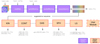 |
Fig. C.1. Flowchart of the NGIST workflow. The purple boxes denote mandatory preparatory modules and the orange boxes denote the optional science modules. The suggested running sequence of the science modules is shown, though we note that the modules may be run in any order. Selected science-ready output .fits files are shown, and we refer to the NGIST documentation for a full list of inputs and outputs. |
Read data (READ_DATA)
Purpose: Read in the input datacube, and return the relevant information as a PYTHON dictionary structure.
Updates since GIST:
• Both GIST and NGIST rely on an input configuration file, within which resides all user-defined options for each module. The GIST version of this file had all variable names on one line, and the values on another, which made editing the correct variable difficult. For NGIST, we have re-written this input configuration file as a YAML, clearly separating out each module, and with one input option per line.
• Added the ability to read in a variance spectrum from the cube if available. This was added to provide the option of non-constant noise for the science routines. If no variance spectra are available, then the variance can be estimated via a DER_SNR algorithm (Stoehr et al. 2008), or a constant noise vector assumed.
• Allowances made for IFS data of different formats, including if the data are in the first HDU, and support for CDELTi keywords.
• Added the ability to perform a Milky Way foreground dust extinction to the input spectra using a Schlegel et al. (1998) correction if an E(B-V) value is provided. This E(B-V) value can be easily calculated using, for example, the SFDQuery routine of the PYTHON dustmaps package.
Spatial masking (SPATIAL_MASKING)
Purpose: Mask spatial regions in an IFS cube. Masks all spaxels below an input minimum signal-to-noise ratio. If specified, will also apply a user-defined mask.
Updates from GIST: None.
Spatial binning (SPATIAL_BINNING)
Purpose: Spatially bin the data to obtain an approximately constant signal-to-noise ratio throughout the field of view. Currently, the only implemented binning routine is the Voronoi technique of Cappellari & Copin (2003), though a user-defined binning scheme can be easily implemented.
Updates from GIST:
• _SPATIAL_BINNING_maps.fits now output, a file that contains maps of the binning scheme, S/N per spaxel, S/N per bin, flux per spaxel, and the number of spaxels per bin.
• KIN and SFH modules now calculate the post-fit signal-to-noise ratio from the residuals and output these in the saved fits files. We use the residual of the data minus the best-fit model to calculate the standard deviation, which is then compared to the mean of the original noise spectrum. The difference between the two values is used to scale the original noise spectrum. The post-fit S/N is defined as the median of the flux divided by the new noise spectrum.
Prepare spectra (PREPARE_SPECTRA)
Purpose: Prepare spectra for analysis by binning them, and then log-rebinning them spectrally. Currently, there is only one routine to perform these tasks, default.py
Updates from GIST: None.
Stellar kinematics (KIN)
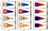 |
Fig. C.2. Comparison of derived stellar kinematic moment maps between GIST and NGIST for galaxy IC 1711. The left column shows GIST output for (from top to bottom) V⋆, σ⋆ (with surface brightness contours overlaid), h3, and h4. The middle column shows the same, but from NGIST, and the right column shows the formal error derived by the PPXF fit of NGIST. For both the GIST and NGIST runs, cubes were binned to S/N = 100 (using the binning maps created by NGIST), and all other input parameters were kept identical. |
 |
Fig. C.3. Direct bin-by-bin comparison of derived stellar kinematic moments from GIST (y-axis) and NGIST (x-axis) for GECKOS galaxy IC 1711. Every point is a Voronoi bin (as shown in Figure A.2), and points are colour-coded by the S/N determined from the residual of the data minus the best-fit model. |
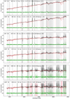 |
Fig. C.4. Comparison of the masking and subsequent PPXF best-fit for three Voronoi bins of the GIST (top) and NGIST (bottom) fits shown in Figures A.2 and A.3. In each case the original spectrum of the bin is shown as a black line. The emission and sky line masks provided to PPXF are shown as the shaded grey regions. NGIST additionally performs further cleaning of the spectra, and these additional clipped regions are shown as shaded red regions. The best fit to the stellar continuum is shown in red, and the residuals in green. The derived stellar kinematic parameters for each spectrum are also listed. |
Purpose: Measure the stellar kinematics of the observed spectra. Currently, there is only one routine implemented, that uses the PPXF method of Cappellari & Emsellem (2004), Cappellari (2017), and Cappellari (2023).
Updates from GIST: A considerable rewrite to the PPXF routine has occurred, including:
• Removed the ability to obtain spatially resolved λr measures and print maps, as this is an integrated quantity.
• Added the option for the user to specify the BIAS value (see PPXF documentation) input to PPXF. If not stated, then the bias is calculated following Cappellari & Emsellem (2004) as
 (A.1)
(A.1)
where Nλpixels is an integer vector containing the indices of the good pixels within the input spectrum (i.e. those to be used in the fit).
• Normalised the input spectrum as suggested by Cappellari (2017)to avoid numerical issues. The output best-fit model is then scaled back to match the original flux of the galaxy spectrum.
• Added the ability to turn the PPXF CLEAN function on or off using the keyword ‘DOCLEAN’. Useful in finding a proper estimate of the noise.
• Included the option to use a multi-step process to determine the stellar kinematics following the method from van de Sande et al. (2017), which can be used when the absolute value of the noise spectrum is uncertain and requires scaling. In this method, to increase the fitting speed for individual Voronoi bins, PPXF is run once on a combined mean spectrum of all Voronoi bins to get a single optimal template. For each Voronoi bin, PPXF is then fitted threetimes:
1) Using a constant noise spectrum. A new estimate of the noise is derived from the residual of the data minus the best-fit model, using a bi-weight estimate of the scale (standard deviation). The approach is described in Hoaglin et al. (1983).
2) Using the scaled noise spectrum from step 1), PPXF is fitted with the single optimal template, this time employing the CLEAN option to clip 3σ outliers from the comparison of the best-fit model to the data.
3) In the final step, we use the updated spectral mask from step 2, the scaled noise spectrum, and the full set of templates.
In Figure A.2, we show the comparison of the stellar kinematic maps from GIST and NGIST for GECKOS iDR1 galaxy IC 1711, with a target S/N = 100 and minimum spaxel S/N = 5. For this test, we adopted the v11.0 EMILES Base models with the BaSTI scaled-solar isochrones, that can be used in both GIST and NGIST. For these fits, we removed the ‘unsafe’ SSPs with metallicities [M/H] = -2.27, -1.79, and +0.40. The wavelength range was set to 4800–8900Å, we assumed a constant noise spectrum, and fixed the PPXF bias value to 0.14.
There is a good agreement in Figure A.2 for the results from GIST (left column) and NGIST (middle column) for all kinematic parameters, though there are noticeable differences in the outer bins where the contribution from the sky lines and telluric absorption features become more dominant. In particular, h3 and h4 reach more extreme values in the GIST maps. A one-to-one comparison of the results are presented in Figure A.3, where the data are colour-coded by the S/N calculated from the residual of the data minus the best-fit. Here σ⋆ can be seen to exhibit some scatter even at moderate values of S/Nresidual.
Even in the central regions, we find subtle but significant differences, best seen in Figure A.4. Here, we present the GIST (upper) and NGIST (lower) spectra from a central bin (#882; x,y = 1,0 [kpc]; top two spectra, highest S/N), a mid-disc bin (#1873; x,y = 5, 0.5 [kpc]; middle two spectra), and an outer bin (#1949; x,y = 9, -0.75 [kpc]; lower two spectra, lowest S/N). For each spectrum in Figure A.4, the original, Voronoi-binned spectrum is shown in black, the PPXF-derived best fit spectrum in red, and the residuals of the fit in green. For both GIST and NGIST runs, the emission and sky line masks employed in the fit are shown as grey-shaded regions.
NGIST includes an additional spectral cleaning step, and the regions masked as a result of this step are shown as shaded pink regions. While the sky line masks are extensive (based on the UVES sky emission atlas, where every sky line of flux > 5 × 10⁻¹⁶ erg s−1 Å−1 cm−2 arcsec−2 was masked), some additional masks are always applied by the NGIST cleaning step. The number of masked spectral pixels as a result of the cleaning step increases from central to outer galaxy regions where sky lines begin to dominate. There are clear regions in the outer bin spectrum that benefit from the additional masking, particularly a region around  , which the Calcium triplet sits on top of at the redshift of this galaxy. We expect this to be the reason behind the scatter in σ⋆ seen in Figure A.3 for a small number of bins. These bins are located around the edges of the galaxy map, where σ⋆, err is at its highest.
The derived kinematic parameters are listed in the top left corner of each spectrum. While there are clear differences between all derived kinematic moments in each case, we refer to Figure A.3 to see these trends in a statistical sense. Generally, the biggest differences are seen for the high-order kinematic moments, in regions where the sky and telluric residuals are significant, and at lower S/N. We find that the added cleaning step of NGIST removes spurious outliers, adding stability and reliability as compared to GIST.
Continuum and continuum-subtracted cube creation (CONT)
Purpose: Create continuum-only (i.e. emission line-subtracted), and continuum-subtracted (i.e. line only) cubes.
Updates from GIST: This is a new module, borne out of the need for these data products within the GECKOS team. This module is closely modelled on the stellar kinematics module, and employs PPXF to model and fit the stellar continuum. The best-fit spectrum in each Voronoi bin is rescaled to the individual spaxel level using the ratio SIGNALbin / SIGNALspaxel, and then subtracted. The continuum-subtracted spectra are then rebinned from the log-rebinned wavelength channels back to the native, linear resolution channels using a cubic spline interpolation. Spaxels without a continuum fit (where the S/N < S/Nmin) are propagated from the original datacube. This technique leaves a baseline jump between fit and unfit regions, which is handled by later processing.
This best fit for each bin is then saved as the continuum data cube. The continuum cube is then subtracted from the raw binned cube to leave just the emission lines, which are saved as the line-only cube.
Emission lines (GAS)
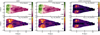 |
Fig. C.5. Comparison of derived stellar kinematic moment maps between GIST and NGIST for galaxy IC 1711. The left column shows GIST output for Vgas (top) and σgas (bottom). The middle column shows the same, but from NGIST, and the right column shows the formal error derived by the PPXF fit of NGIST. For both the GIST and NGIST runs, cubes were binned to S/N = 100 (using the binning maps created by NGIST), and all other input parameters were kept identical. |
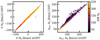 |
Fig. C.6. Direct bin-by-bin comparison of derived Hα gas kinematics from GIST (y-axis) and NGIST (x-axis) for GECKOS galaxy IC 1711. Every point is a Voronoi bin (as shown in Figure A.5), and points are colour-coded by the HαS/N. |
Purpose: Measure the flux, velocity, and velocity dispersion of all defined emission lines.
Updates from GIST: GIST had one routine for emission line measurement, employing GANDALF (Sarzi et al. 2006). We retain this routine, and add two other routines: one of which is a modification to the GANDALF code by the MAGPI team (Battisti et al., in prep), and the other which is PPXF-based. The MAGPI GANDALF modification includes a chi-squared minimization of the local minima by rerunning spaxels that crash (or don’t converge with MPFIT) by adjusting the initial parameter guesses, and then employing a Monte Carlo approach to estimate the flux uncertainties.
To tie the emission line routine in with the PPXF-based routines available for the KIN and SFH modules, and given a significant speedup, we also developed a PPXF-based GAS routine, based on the PHANGS DAP. The input is the raw binned spectrum, and the output of the stellar kinematics module can be used to fix the stellar V⋆ and σ⋆ if desired. As with the GANDALF-based routine, fits can either be performed on a bin level (matching the binning of the previous modules) or on a spaxel-by-spaxel basis. PPXF produces a set of templates, including stellar templates and Gaussian emission lines based on an input line list. There is an option to tie lines together (e.g. the Balmer series), such that their gas velocity will be the same. PPXF simultaneously fits the stellar and gas templates. Gas V and σ are determined, as is the line flux in units of .
.
Figure A.5 compares the Hα velocity and dispersion derived from the GIST GANDALF-based routine (left) to that of NGIST’s PPXF-based routine (right). We note that we do not compare emission line fluxes between the two codes as the GIST emission line module was relatively untested in this respect. Similar to Figure A.3, Figure A.6 compares the binned Hα velocity and dispersion values for the GIST GANDALF-based routine (y-axis) to that of NGIST’s PPXF-based routine (x-axis). There is one clear outlier in the NGIST vs. GIST VHα plot, where the reported GIST VHα = 0. This behaviour is in line with that seen by the MAGPI team (Battisti et al., in prep).
Stellar populations and star formation histories (SFH)
Purpose: Derive non-parametric star formation histories for the observed spectra. Light or mass-weighted averages of stellar age, metallicity, and α-enhancement are also returned.
Changes from GIST: As with the stellar kinematics module, significant changes have been made to the PPXF routine, mostly involving the implementation to a near identical three-step process to better estimate the noise in the input spectrum.
• Added continuum normalisation before fit to avoid numerical issues.
• Added the ability to turn the PPXF CLEAN function on or off using the keyword DOCLEAN. Similar to the KIN module, this is useful in obtaining a proper estimate of the noise.
• Stellar dust absorption E(B-V) maps are now also output, calculated assuming a Calzetti et al. (2000) extinction curve by default, and with no polynomials used in the fit.
• Added the option for using Monte-Carlo (MC) realisations as an alternative to regularisation to obtain stellar population parameters (see for example, Figure 1 of Cappellari 2023, for a comparison between the two techniques). This is an alternative to PPXF regularisation, which has been found to sometimes introduce strong bias in the star formation history (e.g. Wang et al. 2024) We follow the procedures outlined by Pessa et al. (2023) for the PHANGS survey: in each iteration, the input spectrum is perturbed by adding random Gaussian noise with a mean of zero and standard deviation equal to the spectral flux error. The stellar population parameters are calculated from the median of the MC realisations, and uncertainties are then calculated by taking half the difference between 16th and 84th percentiles. There are alternative methods for performing the MC realisations, such as using randomly flipped residuals as error or adding noise to the best-fit spectrum, which could also be available for future updates.
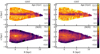 |
Fig. C.7. Comparison of derived mean stellar population properties between GIST and NGIST for galaxy IC 1711. The left column shows GIST output for age (top) and metallicity [M/H] (bottom), whereas the right column shows the results from NGIST. For both the GIST and NGIST runs, cubes were binned to S/N = 100 (using the binning maps created by NGIST), and all other input parameters were kept identical. |
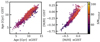 |
Fig. C.8. Direct bin-by-bin comparison of derived mean stellar population properties from GIST (y-axis) and NGIST (x-axis) for GECKOS galaxy IC 1711. Every point is a Voronoi bin (as shown in Figure A.7), and points are colour-coded by the S/N determined from the residual of the data minus the best-fit model. |
We compare the mean stellar population age and metallicity from GIST and NGIST in Figures A.7 and A.8. Similar to Pessa et al. (2023), for this comparison we restrict the wavelength region to 4800-7000Å, and adopt a multiplicative polynomial of order 12. To avoid discrepancies in the derived stellar populations resultant from differences in the stellar kinematic solutions, we adopt the Voronoi binning and stellar kinematics solution from the NGIST SPATIAL_BINNING and KIN modules for both. We apply minimal regularisation to the resultant mean stellar age and metallicity maps. The new cleaning algorithm in NGIST has a significant impact on the derived age and metallicity, most noticeably at large radii and scale heights, where the sky line residuals and telluric correction are most pronounced. We also detect a higher metallicity region in the centre of the GIST metallicity map when compared to NGIST seen in Figure A.7. While at first glance, the higher central metallicities of GIST may be more in line with expectations of inside-out disc galaxy growth, we find that the higher metallicity returned is actually due to a poorer fit. Specific faint lines (for example KI at 7664.9Å and 7690.0Å) are particularly prominent in the central regions of IC 1711 (and indeed can be seen in the central spectra at the top of Figure A.4), but are not present in the SSP models used. For the GIST pipeline, without automatic masking, these lines bias the best-fit PPXF solution toward higher metallicity, while nGIST’s cleaning algorithm identifies them as significant outliers and masks them, resulting in a lower metallicity estimate. A full test of the impact of clipping outliers and the dependence of wavelength range on the mean stellar population parameters is beyond the scope of this paper, but will be explored in future work.
Line strength (LS)
Purpose: Measure the line strength indices from the best-fit continuum spectra and derive stellar population parameters in this manner.
Updates from GIST: None.
Mapviewer
Purpose: GIST also included a quick-look data visualisation tool called Mapviewer. Mapviewer takes the results of a GIST or NGIST run, and displays them in an interactive manner. The user can click on an individual spaxel of an IFS map, and the spectrum, and kinematic, emission line, and stellar population fits are displayed. Any map created by a module can also be displayed, as can the 1D star formation history, and a grid of weights assigned to templates in age/metallicity/alpha space.
Updates from GIST:
• Small cosmetic changes have been made to the Mapviewer interface, providing updated default colour maps and the ability to log-scale emission line fluxes.
• Velocity maps are no longer corrected for the systemic velocity by subtracting the median velocity of the entire map, as this only works when the observations are symmetric and centred on the galaxy centre.
General changes
• Added the ability to use multiple stellar template libraries in the one NGIST call. This will be useful if you for example want to use stellar templates for the stellar kinematics module, and SSPs for the emission lines and stellar populations modules. Currently the MILES, EMILES, and SMILES template sets, the IndoUS template set Valdes et al. (2004), the Xshooter stellar library Verro et al. (2022) and the Walcher et al. (2009) template sets are supported.
• Output: In addition to the output bin table files, we have also created maps fits files for the KIN, GAS, SFH, and LS modules. These maps files are more user-friendly than the original bin table format, as they can be opened and immediately plotted.
Appendix D: Kinematic maps
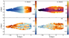 |
Fig. D.10. As for Figure 3, but for ESO 079-003 - BP bulge. |
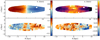 |
Fig. D.11. As for Figure 3, but for ESO 484-036 - BP bulge. |
Appendix E: The effect of wavelength range for fitting stellar kinematics in edge-on galaxies
Given that the amount of light from young vs. old stars and the degree of dust attenuation varies as a function of wavelength in the optical range, the spectral range used for the kinematic fit is important. McDermid (2002) showed that early-type galaxies in the SAURON/ATLAS 3D sample fitting stellar kinematics around the Hβ line (in the blue region of the visible spectrum) yielded information on the kinematics of young stellar discs, whilst the red CaT region provided information on the older stellar disc. While some works have leveraged this observation to infer information on the distribution of stellar populations in relatively face-on galaxies (e.g. Rosado-Belza et al. 2020), in the edge-on case, any variations in derived kinematics (especially in the thin disc regions) are likely due to dust.
In Figure C.1, we present the cautionary tale of derived stellar kinematics for the GECKOS galaxy IC 1711 using a wavelength range around the Hβ-Mg b region (4750–5500 Å, left column), the Calcium II triplet (CaT; 8458-8935 Å, middle column), and the difference in derived stellar kinematics between the two, keeping all other input parameters (including the spatial binning) the same (right column). The differences between the three runs are perhaps most evident in the high-order moment maps. While a strong h3-V⋆ correlation is seen in the inner regions of the disc for all three runs, the small, very central nuclear disc region in which the h3 signal is inverted (resulting in a h3-V⋆ anti-correlation) is only seen in the CaT and full wavelength range maps. We infer that the longer wavelengths are capable of penetrating further into the galaxy disc; the blue wavelengths are attenuated such that we receive diminished kinematic signatures from the galaxy central regions. The result of using stellar kinematic tracers in the blue region for edge-on galaxies (or at least not including enough of the red region) is such that central features of the galaxy may be missed. Indeed, for the above analysis in this paper, we would report IC 1711 as not possessing a nuclear disc.
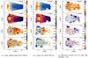 |
Fig. E.1. Stellar velocity (top row), velocity dispersion (second row), h3 (third row), and h4 (fourth row) for GECKOS galaxy IC1711 calculated over the wavelength ranges of Hβ and Mgb (4750–5500 Å; first column), and the CaT (8458–8935Å, middle column) binned to SN = 100. The right column shows the difference between the two. The most obvious feature is seen at the centres of the V⋆ and h3 maps; evidence for a nuclear disc is seen in the CaT maps, but is absent (and presumably hidden by the dust lane) in the Hβ maps. |
Appendix F: Available Spitzer imaging
We present Spitzer 3.6 μm imaging for seven galaxies from the S4G survey (Sheth et al. 2010) in Figure D.1, combined with unsharp-masked images.
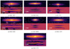 |
Fig. F.1. Spitzer 3.6μm imaging of available GECKOS iDR1 galaxies with an inverse hyperbolic sine (arcsinh) scaling and surface brightness contours overlaid (top), and unsharp-masked images (bottom). The orientation of galaxies here, as throughout, is the same as in Fig 1. |
All Tables
All Figures
|
Fig. 1. g′ri colour images of the sample galaxies reconstructed from the MUSE data cubes of the first 12 galaxies observed as part of the GECKOS survey. In each case, the mosaicked cube has been rotated and aligned such that the photometric major axis is horizontal, and if the dust lane is offset from it, it is always on the lower side of the image. For galaxies not exactly edge-on this means that we look at them from above (i.e. the lower half is the near half) if the dust lane is assumed to be in the mid-plane of the galaxy. The GECKOS pointing strategy was such that the entire (visible) bulge was always included within the MUSE field of view, and at least one side of the galactic disc. Here we show only regions where the signal-to-noise ratio is greater than 2.5; the MUSE field of view often extends further vertically. |
| In the text | |
|
Fig. 2. r-band DECaLS image (top) scaled with an inverse hyperbolic sine (arcsinh) scaling with surface brightness contours overlaid in white (units of r-band magnitude arcsec−2), and unsharp masked image created with a Gaussian smoothing kernel of width σ = 7 − 20 pixels (bottom). Galaxy names marked with a ⋆ are considered to host a boxy-peanut central structure in this work. The orientation of galaxies here, and throughout, is the same as in Fig. 1. |
| In the text | |
|
Fig. 3. Stellar luminosity-weighted line-of-sight velocity, V⋆ (top left), velocity dispersion, σ⋆ (top right, with r-band surface brightness contours overlaid in white), h3 (bottom left) and h4 (bottom right) maps derived with NGIST and binned to S/N = 100 for the galaxy NGC 3279, a galaxy with no obvious visual bulge structure. Galaxies are shown such that the dust lane (and photometric major axis) are oriented horizontally, and such that the dust lane (if offset) is to the lower side of the image. Holes in the maps are regions where bright stars have been masked. Flux contours are overlaid on the σ⋆ maps to highlight the dust lane effects, but not for the V⋆, h3, and h4 maps, to aid in central structure recognition. |
| In the text | |
|
Fig. 4. 1D line profiles, extracted from slits of |
| In the text | |
|
Fig. 5. As in Figure 4, but for the 1D line maps of h3 (left) and h4 (right). The typical median errors are h3, err = 0.016 and h4, err = 0.017. |
| In the text | |
|
Fig. C.1. Flowchart of the NGIST workflow. The purple boxes denote mandatory preparatory modules and the orange boxes denote the optional science modules. The suggested running sequence of the science modules is shown, though we note that the modules may be run in any order. Selected science-ready output .fits files are shown, and we refer to the NGIST documentation for a full list of inputs and outputs. |
| In the text | |
|
Fig. C.2. Comparison of derived stellar kinematic moment maps between GIST and NGIST for galaxy IC 1711. The left column shows GIST output for (from top to bottom) V⋆, σ⋆ (with surface brightness contours overlaid), h3, and h4. The middle column shows the same, but from NGIST, and the right column shows the formal error derived by the PPXF fit of NGIST. For both the GIST and NGIST runs, cubes were binned to S/N = 100 (using the binning maps created by NGIST), and all other input parameters were kept identical. |
| In the text | |
|
Fig. C.3. Direct bin-by-bin comparison of derived stellar kinematic moments from GIST (y-axis) and NGIST (x-axis) for GECKOS galaxy IC 1711. Every point is a Voronoi bin (as shown in Figure A.2), and points are colour-coded by the S/N determined from the residual of the data minus the best-fit model. |
| In the text | |
|
Fig. C.4. Comparison of the masking and subsequent PPXF best-fit for three Voronoi bins of the GIST (top) and NGIST (bottom) fits shown in Figures A.2 and A.3. In each case the original spectrum of the bin is shown as a black line. The emission and sky line masks provided to PPXF are shown as the shaded grey regions. NGIST additionally performs further cleaning of the spectra, and these additional clipped regions are shown as shaded red regions. The best fit to the stellar continuum is shown in red, and the residuals in green. The derived stellar kinematic parameters for each spectrum are also listed. |
| In the text | |
|
Fig. C.5. Comparison of derived stellar kinematic moment maps between GIST and NGIST for galaxy IC 1711. The left column shows GIST output for Vgas (top) and σgas (bottom). The middle column shows the same, but from NGIST, and the right column shows the formal error derived by the PPXF fit of NGIST. For both the GIST and NGIST runs, cubes were binned to S/N = 100 (using the binning maps created by NGIST), and all other input parameters were kept identical. |
| In the text | |
|
Fig. C.6. Direct bin-by-bin comparison of derived Hα gas kinematics from GIST (y-axis) and NGIST (x-axis) for GECKOS galaxy IC 1711. Every point is a Voronoi bin (as shown in Figure A.5), and points are colour-coded by the HαS/N. |
| In the text | |
|
Fig. C.7. Comparison of derived mean stellar population properties between GIST and NGIST for galaxy IC 1711. The left column shows GIST output for age (top) and metallicity [M/H] (bottom), whereas the right column shows the results from NGIST. For both the GIST and NGIST runs, cubes were binned to S/N = 100 (using the binning maps created by NGIST), and all other input parameters were kept identical. |
| In the text | |
|
Fig. C.8. Direct bin-by-bin comparison of derived mean stellar population properties from GIST (y-axis) and NGIST (x-axis) for GECKOS galaxy IC 1711. Every point is a Voronoi bin (as shown in Figure A.7), and points are colour-coded by the S/N determined from the residual of the data minus the best-fit model. |
| In the text | |
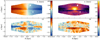 |
Fig. D.1. As for Figure 3, but for IC 5244 - BP bulge. |
| In the text | |
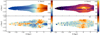 |
Fig. D.2. As for Figure 3, but for PGC 044931 - BP bulge. |
| In the text | |
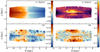 |
Fig. D.3. As for Figure 3, but for NGC 0522 - BP bulge. |
| In the text | |
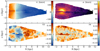 |
Fig. D.4. As for Figure 3, but for IC 1711 - BP bulge. |
| In the text | |
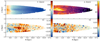 |
Fig. D.5. As for Figure 3, but for NGC 0360 - no obvious visual BP bulge structure. |
| In the text | |
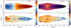 |
Fig. D.6. As for Figure 3, but for NGC 3957 - BP bulge. |
| In the text | |
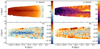 |
Fig. D.7. As for Figure 3, but for ESO 120-016 - BP bulge. |
| In the text | |
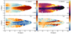 |
Fig. D.8. As for Figure 3, but for UGC 00903 - no obvious visual BP bulge structure. |
| In the text | |
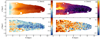 |
Fig. D.9. As for Figure 3, but for NGC 5775 - no obvious visual BP bulge structure. |
| In the text | |
|
Fig. D.10. As for Figure 3, but for ESO 079-003 - BP bulge. |
| In the text | |
|
Fig. D.11. As for Figure 3, but for ESO 484-036 - BP bulge. |
| In the text | |
|
Fig. E.1. Stellar velocity (top row), velocity dispersion (second row), h3 (third row), and h4 (fourth row) for GECKOS galaxy IC1711 calculated over the wavelength ranges of Hβ and Mgb (4750–5500 Å; first column), and the CaT (8458–8935Å, middle column) binned to SN = 100. The right column shows the difference between the two. The most obvious feature is seen at the centres of the V⋆ and h3 maps; evidence for a nuclear disc is seen in the CaT maps, but is absent (and presumably hidden by the dust lane) in the Hβ maps. |
| In the text | |
|
Fig. F.1. Spitzer 3.6μm imaging of available GECKOS iDR1 galaxies with an inverse hyperbolic sine (arcsinh) scaling and surface brightness contours overlaid (top), and unsharp-masked images (bottom). The orientation of galaxies here, as throughout, is the same as in Fig 1. |
| In the text | |
Current usage metrics show cumulative count of Article Views (full-text article views including HTML views, PDF and ePub downloads, according to the available data) and Abstracts Views on Vision4Press platform.
Data correspond to usage on the plateform after 2015. The current usage metrics is available 48-96 hours after online publication and is updated daily on week days.
Initial download of the metrics may take a while.