| Issue |
A&A
Volume 700, August 2025
|
|
|---|---|---|
| Article Number | A102 | |
| Number of page(s) | 15 | |
| Section | Astronomical instrumentation | |
| DOI | https://doi.org/10.1051/0004-6361/202453076 | |
| Published online | 08 August 2025 | |
LISA test-mass charging
Particle flux modeling, Monte Carlo simulations, and induced effects on the sensitivity of the observatory
1
Trento Institute for Fundamental Physics and Applications (TIFPA-INFN),
Trento,
Italy
2
Department of Physics, University of Trento,
Trento,
Italy
3
University of Urbino Carlo Bo, Department of Pure and Applied Sciences (DiSPeA),
Via Santa Chiara, 27,
Urbino
(PU)
61029,
Italy
4
National Institute for Nuclear Physics (INFN), Section in Florence,
Via B. Rossi 1,
Florence
50019,
Italy
5
Max Planck Institute for Gravitational Physics (Albert Einstein Institute),
14476
Potsdam,
Germany
6
OHB Italia SpA Milano,
Italy
★ Corresponding author: This email address is being protected from spambots. You need JavaScript enabled to view it.
Received:
19
November
2024
Accepted:
31
May
2025
Abstract
Context. The Laser Interferometer Space Antenna (LISA) will probe the subhertz spectrum of gravitational-wave emission from the Universe. The space environment causes charge accumulation on its free-falling test masses (TMs) through galactic cosmic rays (GCRs) and solar energetic particles (SEPs) that impinge on the spacecraft. Primary and secondary particles that are produced in the spacecraft material eventually reach the TMs, where they deposit a net positive charge that fluctuates in time. This work is relevant for any current or future space missions that, like LISA, use free-falling TMs as inertial references.
Aims. The coupling of the TM charge with the native stray electrostatic field produces noisy forces on the TM that can limit the performance of the LISA mission. Precise knowledge of the charging process allows us to predict the intensity of these charge-induced disturbances and to design specific countermeasures.
Methods. We present a comprehensive toolkit that allowed us to calculate the TM charging time-series in a geometry representative of the LISA mission, and the associated induced forces under different conditions of the space environment by considering the effects of short and long GCR flux modulations and SEPs.
Results. We studied the impact of spurious forces associated with the TM charging process on the sensitivity of the mission for the gravitational-wave detection for each of the conditions described above.
Key words: elementary particles / instrumentation: interferometers / Sun: particle emission / cosmic rays
© The Authors 2025
 Open Access article, published by EDP Sciences, under the terms of the Creative Commons Attribution License (https://creativecommons.org/licenses/by/4.0), which permits unrestricted use, distribution, and reproduction in any medium, provided the original work is properly cited.
This article is published in open access under the Subscribe to Open model. This email address is being protected from spambots. You need JavaScript enabled to view it. to support open access publication.
1 Introduction
The Laser Interferometer Space Antenna (LISA) (Amaro-Seoane et al. 2017; Colpi et al. 2024) has been adopted by ESA in January 2024 and is scheduled for launch in 2035. It aims to open a window on the millihertz band for gravitational-wave observation. LISA will use free-falling test masses (TMs) that are hosted on a constellation of three spacecraft (S/C) in triangular formation in orbit around the Sun as end mirrors of a large space interferometer with arms extending for 2.5 million km. The LISA TMs are 46 mm cubes of a gold-platinum alloy with approximately 800 nm of gold coating, and they will each follow a geodesic orbit with stray acceleration noise below 3 fm s−2 Hz−1/2 at 1 mHz. Without mechanical contact and a vacuum gap of several millimeters, the TMs are surrounded by a gold-coated electrode housing (EH) that is used for position sensing and actuation (Antonucci et al. 2012a).
High-energy particles of Galactic and solar origin charge the LISA TMs, which makes them sensitive to Coulomb forces through the stray electric fields that are found between the masses and the surrounding EH (see for details Antonucci et al. 2012a). These Coulomb forces a) contribute to the acceleration noise of the TMs by the intrinsic time fluctuations of the deposited charge and the stray electric fields and b) generate spurious signals in the LISA sensitivity band during space weather events. They include solar energetic particle (SEP) events and Forbush decreases (FDs, Forbush 1937, 1954, 1958; Armano et al. 2018a, 2019; Grimani et al. 2020a), sudden depressions in the galactic cosmic-ray (GCR) flux observed at the passage of interplanetary counterparts of coronal mass ejections (ICMEs).
The charging process is associated with energetic particles that can penetrate about 16 g cm−2 of LISA payload and spacecraft shielding material surrounding the TMs (Vidano et al. 2022). This corresponds to a minimum energy threshold of approximately 100 MeV, 20MeV, and 100 keV for hadrons, electrons, and photons, respectively, of galactic and solar origin that penetrate or interact with the spacecraft (Grimani et al. 2024). The charging process is primarily characterized through the evaluation of two fundamental parameters (see the proper definition in Eqs. (4) and (5); Section 4): λNET, which indicates the rate at which the TMs accumulate charge, and λEFF, which is the effective single-charge Poissonian event rate associated with the TM charge noise (Araújo et al. 2005).
Monte Carlo simulations of the charging of the TMs of LISA Pathfinder (LPF), which is the LISA technological demonstrator, were carried out with the codes FLUKA (Battistoni et al. 2014; Böhlen et al. 2014; Vlachoudis 2009) and GEANT4 (Agostinelli et al. 2003; Allison et al. 2006, 2016) before the mission was launched at the end of 2015. These simulations produced very similar predictions for the TM charging rate and noise at solar minimum conditions, although different nominal energy thresholds for electron propagation were considered in GEANT4 (250 eV) and FLUKA (1 keV) (Araújo et al. 2005; Wass et al. 2005; Grimani et al. 2015). This evidence was initially only explained in terms of the average ionization potential in gold that limited the hadron ionization to 790 eV in GEANT4 (Villani et al. 2020; Taioli et al. 2023).
The mission pre-launch work reported by Grimani et al. (2015) was carried out on the basis of predictions of the solar modulation between the end of 2015 and the beginning of 2016. The results of Monte Carlo simulations carried out with these updated predictions were compared to the LPF TMs charging measurements carried out in space on April 20–23, 2016 (Armano et al. 2017, see Table 1). The measured net charging appeared to lie in the middle of the prediction range, while the effective charging was three to four times higher than expected. Moreover, it was observed that the net charging depended on the potential of the TMs (VTM), which saturated to zero for VTM ≈ 1 V (Armano et al. 2023). This observational scenario can be attributed to particles with the same charge sign that enter and escape from the TM in approximately equal number and thus contribute to the charging noise, but not to the net charging. Low-energy electrons (LEE; with E<1 keV) that are produced at the gold surfaces of the TM and EH were the most plausible candidates to explain the observations, as originally suggested by Araújo et al. (2005). The Monte Carlo simulations at that time were not able to account for these LEE because the production and propagation of secondaries was limited below 250 eV for GEANT4 (1 keV for FLUKA).
After the mission, the simulations were refined by incorporating the actual solar modulation of the GCR flux observed during the mission elapsed time (Grimani et al. 2022; Wass et al. 2023) and extending the FLUKA electromagnetic physics below 1 keV. To achieve this, the low-energy ionization (LEI) Monte Carlo program was developed at the University of Urbino Carlo Bo (Villani et al. 2020; Grimani et al. 2022; Villani et al. 2024a). Studies (Grimani et al. 2020b; Villani et al. 2021) demonstrated that ionization is the primary contributor to TM charging, with kinetic emission (LEE emission from surfaces bombarded by keV-MeV particles) and quantum electron diffraction below 100 eV also playing significant roles. Photon-related processes, such as transition radiation, bremsstrahlung, and Čerenkov radiation, were found to be not relevant (Grimani et al. 2020b). In LEI, low-energy ionization was implemented using the Cucinotta formula (Cucinotta et al. 1996), while Sakata cross-sections were applied for electrons and positrons (Sakata et al. 2016). Kinetic emission was initially implemented using Schou’s formalism (Schou 1980; Grimani et al. 2020b), but it was later found to be overestimated by 30% (Grimani et al. 2022) and thus refined using an ab initio approach (Taioli et al. 2023). The quantum electron diffraction model, initially assumed for particle normal incidence, (Grimani et al. 2022) was updated to account for electron direction and Bragg’s planes at energies below 100 eV (Villani et al. 2024a). The TM charging obtained with FLUKA-LEI simulations reproduced the observations carried out with LPF well (Grimani et al. 2022; Villani et al. 2024a).
Under the ESA contract 4000133571/20/NL/CRS (Test mass charging and LPF lessons learned) we started the development of the TM charging toolkit (TMCTK) in 2021. This was based on GEANT4 to study the TM charging for LPF/LISA-like GRS featuring the low-EM physics learned with FLUKA-LEI (see Section 2), a general modeling of the particle fluxes (described in Section 3), and the analysis of the charging process effect on the mission performance (see Sections 4, 5, and 6). The TMCTK was finally delivered to ESA in 2023 and adopted version 11 of GEANT4 (released in December 2021) along with an improved version of the GEANT4-DNA module (Incerti et al. 2010a,b, 2018; Bernal et al. 2015; Tran et al. 2024), which was made to address the simulation of extremely low-energy electromagnetic processes (down to 10 eV) that are typically used for radiobiology studies (Sakata et al. 2018).
The first aim of this paper is to present the main elements of TMCTK and its first results for the LISA mission, which allow us to accurately predict the impact on the LISA mission of a wide array of environmental charging scenarios. Despite the improvements, however, the TMCTK prediction for the charging noise λEFF appears to be underestimated with respect to FLUKA-LEI and LPF observations. Further investigations of this issue revealed major discrepancies between TMCTK and FLUKA-LEI for some particular aspects of LEE propagation such as backscattering and the transmission yields on the gold slabs. The details of these discoveries are discussed in Section 5 and will be the subject of future investigation together with the GEANT4 scientific community.
Net and effective TM charging and TM equilibrium potential measured with LPF (Armano et al. 2017, 2023).
2 LISA test-mass charging Monte Carlo simulation
The effects of the space environment on the LISA TM charging with the TMCTK were estimated based on the Monte Carlo simulation of the particle-to-matter interaction.
The TMCTK features GEANT4 with a user interface that allows us to set the simulation time span and to choose the species of the interacting particles and their energy spectra parameterized as described in Section 3. The user can also select predefined case studies from a screen menu. The geometry of the simulation and the physical processes involved are encoded in GEANT4. The CPU time per single core (Xeon 2.2 GHz) is about 5 × 10³ events per second for protons.
We considered four concentric spherical aluminum shells that surround a gold cubic TM to represent the material distribution in the LISA S/C (see Figure 1). This material amount was quantified in a total of 16 g/cm2, mainly concentrated in the vicinity of the TM. This is a highly simplified model of the matter distribution. The amount of matter was set on the basis of a preliminary design of the LISA spacecraft (Vidano et al. 2022). The adoption of a simplified geometry is common practice1 in the design process of space missions to estimate the effects of the space environment on sensitive parts of the satellite (Vocca et al. 2004). Moreover, given the importance of the emission of secondary particles generated by particle interaction in the immediate vicinity of the TM, the innermost interface of the GRS EH was modeled as a cubic gold box of 150 nm and 5.2 cm on the side to represent part of the outer film of gold, which is separated from the TM itself by a 3 mm vacuum gap. This arrangement was also adopted by Taioli et al. (2023) and allowed us to save computation time without losing the significance of the simulation. The thickness of the layer was chosen to be conservatively greater than the mean free path of electrons with energies below 100 eV. Extensive studies of the output of the simulation demonstrated that the results depend only weakly on this parameter.
Particle propagation in GEANT4 occurs in discrete steps that are selected on the basis of the active processes. In particular, the active processes characterized by high cross-sections for an assigned material and particle energy have a higher probability to be selected by the simulation engine. The length of the propagation step depends on the selected physical process, but can also be limited by the user to a custom value. The particle ionization energy loss is implemented according to the continuous slowing-down approximation (CSDA). After each step, the energy of the simulated particle is lowered accordingly. In general, this approach allows a reliable description of the production of secondaries and of the particle energy loss over the step length by maintaining a relatively high efficiency from the point of view of the computation power.
GEANT4 allows for a modular handling of the different categories of physical processes (electromagnetic, hadronic, and decay) that can be activated independently in the simulations. These modules are included in a modular physics list in which each process uses appropriate theoretical models for a given energy and material that can be chosen by the users. Activating a large number of modules increases the precision of the simulations and the number of possible considered interactions at the cost of a major increase in the processing time. The physics list we implemented for this study was the standard QGSP-BIC (Geant4 Collaboration 2024), which includes all the principal electromagnetic and hadronic processes as well as radioactive decay and neutron transport. Of particular interest for us was the implementation of the module that activates the electromagnetic interactions. In our simulations, we made use of the G4StandardEM-option4 (Opt4) module (Ivanchenko et al. 2014), which is particularly well suited for studies in which electrons and positrons play a relevant role. The module allowed us to track these particles down to energies of 100 eV. Opt4 was used in all spacecraft regions, except for the outer 150 nm of gold of the TM and EH, where the QGSP-BIC physics list was integrated with the GEANT4-DNA module to account for the production and propagation of LEE. The processes we implemented in the simulation are briefly described in the following subsections.
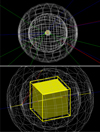 |
Fig. 1 Top panel: LISA spacecraft simplified matter distribution around the TM. Bottom panel: magnified view of the central part of the geometry modeling the GRS and the TM in GEANT4. The 150 nm wide cubic box that models the last interface of the EH and the spherical shielding shells are visualized in wireframe mode for visualization purposes. |
2.1 Simulation of low-energy electrons
GEANT4-DNA replaces the comprehensive multiple scattering processes of Opt4 with more detailed models for LEE interactions, including elastic scattering, electronic excitation, ionization, vibrational excitation, and molecular attachment.
For electrons in gold, GEANT4-DNA includes specific cross-section models covering energies from 10 eV to 1 GeV. Although GEANT4-DNA can also simulate processes involving nuclei, such as protons and α particles, no cross-section models for these particle interactions in gold are currently available. We therefore implemented the custom processes described in Section 2.2, analogously to Wass et al. (2023), to model LEE kinetic emission following the impact of these particles. They contribute minimally to the overall LEE production, however.
GEANT4 allows for the propagation of electrons until their energy is reduced by CSDA below a threshold Emin, which for the GEANT4-DNA module was set at 10 eV by default. Below this threshold, the propagation of the particle was stopped. The discrete interactions have a different low energy threshold Eth that encodes the energy validity range of their cross-section models. In GEANT4-DNA, Eth was nominally set at 10 eV as Emin. The minimum energy required for an LEE to escape from the gold surfaces of the TM and EH is equal to the gold work function, however, which is found to be typically in the range 3.9–5.2 eV (Wass et al. 2023). In our toolkit, the Emin threshold was therefore lowered to 4 eV, and (Eth) was not altered. This adjustment allowed secondary electrons with energies between Emin and Eth to reach the gold-vacuum boundary to escape from the surface.
As demonstrated by Taioli et al. (2023), this approach effectively reproduces the theoretical and measured electron back-scattering yield of gold. When we varied the Emin threshold between 3.8 and 4.2 eV, we found no significant impact on the λNET and λEFF.
2.2 Low-energyelectrons from hadrons
Kinetic emission of LEEs can also occur when nuclei, such as protons and α particles in the keV-MeV energy range, interact with the gold surfaces of TMs and EHs. Since cross-section models for these processes in gold are not included in GEANT4-DNA, two custom processes were implemented in the GEANT4 physics list. These processes simulate the emission of secondary LEEs using a yield-based approach that is triggered when protons or α particles traverse the gold surfaces. The number of generated electrons, Y(E,θ), as a function of proton energy E and incidence angle θ with respect to the normal to the surface was sampled from the average proton and α kinetic emission yield function. This function is defined by the following formula (Furman & Pivi 2002; Wass et al. 2023):

where
![Mathematical equation: ${E_{max}}\left( \theta \right) = {E_0}\left[ {1 - 0.7\left( {1 - \cos \left( \theta \right)} \right)} \right]$](/articles/aa/full_html/2025/08/aa53076-24/aa53076-24-eq3.png)
and
![Mathematical equation: ${Y_{max}} = {Y_0}\left[ {1 + 0.66\,{{\cos }^{0.8}}\left( \theta \right)} \right].$](/articles/aa/full_html/2025/08/aa53076-24/aa53076-24-eq4.png)
In the above formulas, Y0 is the value of the yield for particles that are normally incident on the surface, E0 represents the peak energy of the distribution, and s is its spectral width. In the case of protons, values of Y0 = 2.18, E0 = 180 keV and s = 1.54 were used (Furman & Pivi 2002). For the kinetic emission given by α particles, which is very subdominant with respect to the electron production from protons, the angular dependence was considered to be constant, and values of Y0 =6, E0 = 200 keV and s=1.64 were used. The energy distribution of the LEE produced by these processes was sampled from a narrow (σ = 2 eV) distribution centered around 8.4 eV, and their emission direction was assumed to be isotropic with respect to the surface normal direction.
Figure 2 shows the yield functions of the LEEs generated by kinetic emission from protons and helium nuclei (α particles) as implemented in the toolkit.
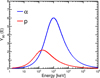 |
Fig. 2 Low-energy electron yield of the kinetic emission processes for protons (p; red) and α particles (blue) that perpendicularly cross the gold surfaces (Y90) as a function of p and α energy. |
2.3 Electron quantum diffraction
Some of the electrons involved in the TM charging process have low energy; therefore, the wave-like quantum mechanical behavior of these particles, such as diffraction, cannot be disregarded.
Diffraction occurs when the wavelength of the electron is comparable to the spacing between the atoms in a crystal lattice (≈4 Å for gold). In order to calculate the probability of diffraction at a given electron energy E, the radial Schrödinger equation of an electron in the potential of the crystal lattice must be solved,
 (1)
(1)
where Z is the atomic number (Z = 79 for gold), m is the electron mass, l is the angular momentum quantum number, and Vex(r) is the exchange potential that arises because electrons are identical particles. Finally, Rl(r) is the radial wavefunction.
The Schrödinger equation (1) was solved in two different ranges: inside the potential of a single ion, and in the region between atoms, where the potential is constant. The two solutions were matched by imposing that they assume the same value at the boundary of the two regions and that their derivatives are continuous. With this approach, we estimated the electron reflection probability (for the details of this procedure, see Van Hove et al. 1986; Grimani et al. 2020b; Villani et al. 2024a).
The theoretical calculation described above provides the electron backscattering probability as a function of electron energy and incidence angle with respect to the normal of the gold surface due to quantum diffraction. The GEANT4 toolkit was integrated with this custom process active only in proximity to the two facing surfaces of TM and EH, similarly to the process described in Section 2.2. The incoming electron was reflected back at the same incidence angle, according to the estimated quantum backscattering probability, without an energy change.
3 Modeling the space particle environment for LISA
The LISA TM charging will depend on the overall particle flux incident on each spacecraft. Given the about 16 g cm−2 (Vidano et al. 2022) of spacecraft material that are expected to shield the TM on board the three LISA spacecraft, only primary particles above a certain energy threshold will contribute to the charging. These limits are about 100 MeV/n for hadrons, 20 MeV for electrons, and 100 keV for photons (Grimani et al. 2024). The LISA observatory is expected to nominally operate for 4.5 years and up to 10 years. To fully encompass the variability in the environmental conditions during this period and to evaluate the range of the net charging and charging noise that plausibly will be observed, we considered different conditions of the interplanetary medium: long- and short-term variations in the GCR fluxes, and real SEP events of different intensity.
In general, GCR fluxes and solar particles associated with gradual events (Reames 2021, 2022) lie in the energy range of interest for the TM charging, and their energy dependence must be taken into account to properly assess the TM charging. The composition of GCR consists of approximately 90% protons, 8% helium nuclei, 1% heavy nuclei, and 1% electrons. The percentages are meant in particle numbers to the total number (Simpson 1983; Papini et al. 1996). Conversely, the particles of SEP events are mainly protons (99%), and electrons and nuclei constitute the remaining 1% (Reames 2021).
TMTCK simulated the different fluxes according to the parameterization we discuss in the following subsections.
3.1 Long-term variations in Galactic cosmic rays
Long-term variations in the cosmic-ray intensity (>1 month) show quasi-11 and quasi-22-year periodicities associated with the solar activity and the polarity change in the global solar magnetic field (GSMF). During the past three solar cycles, the overall GCR flux above 100 GeV has been observed to vary by a factor of four in the inner heliosphere (Grimani et al. 2023b, 2021, 2023a).
LISA is expected to be launched in 2035 near the maximum of solar cycle 26 during a positive-polarity period of the GSMF, which is the same as for LPF. Grimani et al. (2008) showed that during positive-polarity periods, the energy spectra, J(r, E, t), of cosmic rays at a distance r from the Sun at a time t are well represented by the symmetric model in the force-field approximation by Gleeson and Axford (G&A, Gleeson & Axford 1968). These authors found that by considering time-independent interstellar cosmic-ray spectra J(∞, E + Φ) and an energy-loss parameter Φ, J(r, E, t) can be expressed as follows:
 (2)
(2)
where E and E0 represent the total energy and rest mass of the particle, respectively. For Z=1 particles with a rigidity (particle momentum per unit charge) higher than 100 MV/c, the role of the solar activity was taken into account by defining a solar modulation parameter ϕ measured in MV/c, which is equal to Φ (Armano et al. 2018a) at these energies.
The proton interstellar spectrum by Burger et al. (2000) was adopted to set the solar modulation parameter estimated by Usoskin et al. (2011, 2017) and was used here2. Unfortunately, Burger et al. (2000) provided no helium flux at the interstellar medium. As a result, we used the Shikaze et al. (2007) helium interstellar spectrum, selected on the basis of the BESS experiment data. In order to test the reliability of the model and of our approach for proton and helium flux estimates, we compared the outcomes of the model to the monthly average space-station magnetic spectrometer experiment AMS-02 data gathered in 2016 above 450 MeV/n (Aguilar et al. 2021). While the model outcome and data for proton flux agree within 10%, the helium flux obtained with the model was higher by 25% than the data. We therefore normalized the helium flux for LPF in 2016 to the contemporaneous AMS-02 data gathered above 450 MeV/n. For LISA, we considered the same approach because the LISA particle detectors will provide proton and helium differential fluxes up to 400 MeV/n.
The modulated particle spectra obtained with the G&A model were parameterized according to the following equation (Papini et al. 1996):
 (3)
(3)
where the parameter b measured in GeV(/n) was used to depress the particle flux at low energies, and the dimensionless parameters α and β allowed us to reproduce the trend of the spectrum at high energies. Finally, A, measured in particles/(m2 sr s (GeV(n−1))−α+β+1), is the normalization constant. The agreement between Equation (3) with the G&A model was discussed in detail by Armano et al. (2019).
Since the solar activity is not yet known for the time at which LISA will be in orbit, we considered a solar modulation parameter of ϕ=200 MV/c at solar minimum and ϕ=1200 MV/c at solar maximum as extreme cases for all particle species on the basis of previous observations of the solar modulation parameter. In Figure 3 and Table 2, we present our estimates for proton and nucleus energy spectra and the associated parameterization according to Eq. (3) for LISA.
The galactic and interplanetary electron contribution to the LPF TM charging was discussed in detail by Grimani et al. (2009). For LISA, we also only considered galactic electrons, and we disregarded electrons below ≃20 MeV, which typically have an interplanetary and solar origin. The electron flux at the interstellar medium by Moskalenko & Strong (1998) adopted here (dotted line in Figure 4) was found to reproduce observations gathered near Earth at solar minimum, maximum, and during different epochs of the GSMF better than others (Grimani 2004, 2007). The G&A model was also used to modulate the electron interstellar spectrum at 1 AU at solar minimum (ϕ=200 MV/c; dashed line in Figure 4) and at solar maximum (ϕ=1200 MV/c; continuous line in Figure 4). The parameters in Eq. (3) for electrons are shown in Table 3.
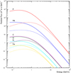 |
Fig. 3 From top to bottom: Proton (p, red), helium (He, blue), carbon (C, magenta), oxygen (O, green), nitrogen (N, cyan), and iron (Fe, yellow) cosmic-ray energy spectra at solar minimum (ϕ = 200 MV/c; continuous lines) and solar maximum (ϕ = 1200 MV/c; dashed lines) as extreme conditions for LISA. |
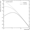 |
Fig. 4 Galactic electron energy spectra at solar minimum (dashed line) and solar maximum (continuous line) for LISA. The interstellar spectrum is represented by the top dotted line (Moskalenko & Strong 1998). |
Parameterizations of energy spectra of protons and nuclei at 1 AU for LISA.
Parameterization of electron energy spectra above 20 MeV at solar minimum and solar maximum.
3.2 Short-term variations in Galactic cosmic-rays
Short-term variations in Galactic cosmic-rays (<1 month) are observed when interplanetary structures pass through the spacecraft’s orbital path. In particular, short-term variations in the GCR flux are called recurrent FDs when they are associated with the passage of high-speed solar wind streams, and they are called nonrecurrent FDs (or simply FDs) when they are generated by ICMEs (Forbush 1937, 1954, 1958). Detailed studies of the interplanetary physics of GCRs have been carried out with LPF for LISA in Armano et al. (2018a, 2019); Grimani et al. (2020a); Villani et al. (2023).
The recurrent short-term variations last for 9.1 days on average and the particle energy dependence below a few GeV is marked, while intense FDs may present an energy dependence up to tens of GeV. It is often hard to study the energy dependence of FDs because solar particles are simultaneously present. As case studies, we chose to consider one recurrent FD observed with LPF and one nonrecurrent FD that was observed in space with the PAMELA experiment (Adriani et al. 2011) and on the ground with neutron monitors. The method for calculating the particle flux parameterization during these events was described in Armano et al. (2018a, 2019), and Grimani et al. (2020a). We were able to use both PAMELA and neutron monitor observations for the proton flux estimate because PAMELA was in orbit near Earth (see Villani et al. 2024b). The evolution of the proton flux during the FD was estimated at the onset (December 14, 2016, 15:39 UT), for which we considered the undisturbed proton flux measured on November 2006, as suggested by Adriani et al. (2011), in the mid-phase at 17:20 UT, and at the deepest point at 24:00 UT of the same day. The proton fluxes that were observed during these events and their parameterization are reported in Figures 5 and 6 and in Tables 4 and 5.
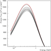 |
Fig. 5 Recurrent short-term variations of GCRs observed with LPF between November 21 and December 4, 2016. The continuous lines indicate the decrease phase, and the dashed lines show the recovery phase. The top continuous red line indicates the proton energy spectrum at the onset of the event. |
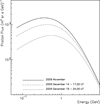 |
Fig. 6 Forbush decrease observed on December 14–15, 2006 with the PAMELA experiment in space and on Earth with neutron monitors. |
Parameterizations of the proton energy spectra during a recurrent variation in the proton-dominated flux measured with LPF between November 20 and December 4, 2016.
Parameterizations of the proton energy spectra during a Forbush decrease observed on December 14–16, 2006.
3.3 Solar energetic particle events during LISA
The charging of the TM is expected to increase by several orders of magnitude during SEP events (Grimani et al. 2022) with respect to the background values associated with the continuous flow of GCRs. This process is sensitive to hadrons above 100 MeV(/n) and is affected by gradual events that are characterized by proton acceleration above 50 MeV. During the evolution of gradual SEP events, particles vary in space, energy, and time from the onset to the decay. At the onset, the solar particle energy spectra most likely show a power-law trend with an exponential cutoff, while at the peak, a power-law trend is observed in the majority of cases. The proton spatial distribution is characterized by varying pitch-angle distributions. We recall that the pitch angle is defined as the angle between the particle velocity and the nominal direction of the interplanetary magnetic field (Parker spiral). At the onset of the events, the particles mainly propagate along the interplanetary magnetic field lines, while during the late phases, the arrival direction becomes isotropic. Because we considered an isotropic matter distribution in the spacecraft for the LISA simplified geometry, we did not consider the evolution of the SEP spatial distribution in the Monte Carlo simulations. The parameterization of the solar particle energy spectra during the event dynamics was discussed, for instance, by Grimani et al. (2013).
Solar electrons have been demonstrated to play a minor role in affecting the TM charging and will not be detected by the LISA radiation monitors according to the current design (Mazzanti et al. 2023). As a result, even if solar electrons were to reach the LISA S/C before protons due to velocity dispersion, no short-term forecasting of SEP events will be allowed on board LISA.
For events that are magnetically well connected to the active region of the Sun in which the solar eruption occurred, the particle flux can increase by several orders of magnitude in 15 minutes on the three LISA satellites. The average duration of medium to strong SEP events (fluence > 106) is about 1.5 days, although some events can last up to 5 days (Shaul et al. 2006; Rodríguez-Pacheco et al. 2020).
From the standpoint of the TM charge measurement, it is unfortunate that no SEP events were observed above the GCR background during the LPF operations. As a result, the TM charging during SEP events can be only estimated with Monte Carlo simulations for LPF and LISA (Grimani et al. 2022). We considered the onset and peak of gradual SEP events with different intensities. In particular, we studied two SEP events with a different fluence: the peak of the event on September 29, 1989 (fluence 107–108 protons cm−2, Miroshnichenko et al. 2000), and the event observed by the PAMELA experiment in space on December 13, 2006 (fluence between 106 and 107 protons cm−2 Adriani et al. 2011). The proton fluxes observed during these events are shown in Figure 7.
Data from the Solar Orbiter mission (Müller et al. 2020; García Marirrodriga et al. 2021; Rodríguez-Pacheco et al. 2020)3 on SEP event occurrences above 70 MeV will allow us in the near future to investigate the effects of several other event dynamics on LISA in detail. We stress that SEP events with fluences of 105–106 protons cm−2 are not observed at solar minimum above the background of GCRs above 70 MeV. On the basis of observations gathered during past solar cycles, about 10 SEP events per year at most are expected during the LISA operations during the first part of the mission because the LISA launch is scheduled for the maximum of solar cycle 26 (Singh & Bhargawa 2019).
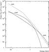 |
Fig. 7 Solar energetic proton fluxes observed during the evolution of the gradual events on September 29, 1989 (dashed line), and December 13, 2006 (continuous line). The different phases of the events are indicated. The timings of the events shown in the figure appear in Table 7. |
4 Case studies of LISA test mass charging
In space, the deposit of a charge on the TMs is an inherently Pois-sonian process. Each deposit j, that is, one elementary charge or more, of either signs, has its rate λj. The TMs charge up with a rate
 (4)
(4)
This charging process produces shot noise  on the TMs with the current I = λEFF e, where
 (5)
(5)
The integral of the charging yields the red power spectral density of the deposited charge SQ = 2λEFF e2/(2πf)2 as a function of the frequency f (Araújo et al. 2005).
The LISA observatory measures the relative motion of TM pairs in the 0.1 mHz to 1 Hz band (Amaro-Seoane et al. 2017; Colpi et al. 2024). The calculation of the λNET and λEFF must therefore be representative at timescales of 1000 seconds or more for the galactic cosmic-ray flux.
Figure 8 illustrates the distributions of λNET and λEFF obtained with a series of ten independent runs as a function of the simulation time. The proton flux at solar minimum (ϕ = 200 MV) was considered as a reference case. The dispersion on λNET steadily decreases around a constant central value. In the case of λEFF, the contribution of large deposits that rarely occur due to the power-law nature of the CR energy spectrum is boosted by its square dependence on the deposit itself (see Eq. (5)), and for the same reason, it is not counterbalanced by any negative contribution. As a result, the distribution of λEFF displays occasional large positive outliers for shorter simulations based on a limited number of rare large charge-transfer events, as well as many slightly below average values of λEFF. These effects are washed out in longer simulations.
The figure clearly shows that a good convergence of the results, especially for λEFF, can only be obtained with simulation times above 103 s for protons. We set the simulation time for protons conservatively to 104 s at solar minimum and maximum. This minimum simulation time was further increased for rare particles in cosmic rays, such as nuclei and electrons. The simulation time we used for the various species is reported in the second column of Table 6.
In the top panel of Figure 9, we report as an example the contributions to λNET and λEFF as a function of the energy of primary protons at solar minimum. The λNET decreases abruptly above 1 GeV. The meaning of this sharp decrease can be inferred by observing the breakdown of the contribution of the different secondary particle species generated by the interaction of the primary protons that appear in the bottom panel of the same figure. Below 200 MeV, the λNET is dominated by protons that stop in the TMs. The production of positively and negatively charged pions (shown in the figure) above this energy tags the occurrence of hadronic interactions in the body of the TM (minimum traversed gold material grammage 91 g cm−2). More secondary particles escape from the TM than penetrate from outside. The escaping negatively charged particles charge the TM positively, and the opposite occurs for positively charged particles. The electron curve is also affected by an additional production of electrons by particle ionization, however. We point out that globally positive and negative pions, electrons, and positrons contribute only little to the total charging with respect to protons.
The trend of λEFF as a function of the primary proton energy shows contributions that peak for primary proton energies in the GeV range and receive significant contributions that span from 150 MeV to 50 GeV (see Figure 9). Charge deposits of opposite signs sum up quadratically in the λEFF formula (Eq. (5)) and do not cancel out.
The discussions reported above allowed us to properly set the simulation time frame for all particle species that contribute to the TM charging, as discussed in Section 3. As an example of TM charging time series, we report in Figure 10 the Monte Carlo simulation results obtained for primary protons and iron nuclei under the same solar modulation conditions (ϕ=200 MV/c). The two timeseries exhibit a prevalence of positively charge deposits that reach values of several hundred elementary charges per second deposited on the TM. As expected, these events are significantly more frequent in the iron case because the overall number of electrons that are generated by ionization scales with the square of the particle charge.
This evidence emerges more clearly in the charging his-tograms4, shown in the right panel of the same figure, where the occurrence of large charge deposits is consistently higher for the iron nuclei.
Figure 11 (top panel) presents a comparison between the charging histograms obtained from two proton simulations at extreme solar minimum (ϕ = 200 MV/c) and solar maximum (ϕ = 1200 MV/c) conditions. The deposit rates (see top panel of Figure 11) are consistently lower for solar maximum fluxes. This imbalance fades out for increasingly higher charge deposits because solar maximum fluxes are relatively poor in low-energy particles compared to solar minimum fluxes.
A global charging histogram from a complete GCR flux simulation of 10 000 seconds at extreme solar minimum (ϕ = 200 MV/c) is presented in Figure 11 (bottom panel), broken down by contributions from each simulated particle species. Only species with the highest expected contributions were simulated, using the flux parameterization discussed in Section 3. The peak of the distribution, which mainly determines the net charging, is dominated by proton and helium contributions, while the tails, which mostly affect λEFF, are populated by other particle species in a more than proportional way with respect to their relative abundance.
The results regarding λNET, λEFF, and their respective uncertainties obtained with TMCTK in different space environment conditions and for different particles are reported in Table 6. This table clearly shows that the dominant contribution to the total λNET and λEFF comes from primary protons. Nuclei contribute less in general, but relatively much with respect to the abundance of these particles in GCRs. This is particularly evident for iron nuclei, which contribute ~10% to the total λEFF due to the combined effects of its high Z and relative abundance with respect to other heavy nuclei. The electrons, which only constitute 2% of the CGR sample, also contribute ~10% to the total effective charging. Moreover, this particle species alone shows a marginally negative contribution to λNET.
In Figure 12 (top and bottom panel) and Table 7, we present the time evolution of λNET and λEFF for the recurrent short-term variation appearing in Figure 5 and for the nonrecurrent shown in Figure 6. In Table 7 we also report the results for the simulation of two SEP events on September 29, 1989, and December 13, 2006 (see Figure 7). For the SEP events, we carried out simulations for a fixed duration of 6 seconds given their rapid evolution and their extremely high flux with respect to GCRs. Figure 12 (middle panel) also shows the time evolution of λNET and λEFF for the December 13, 2006, SEP. The λNET appears to follow the variations in the input fluxes that are dominated by the primaries that stop inside the TM. This correlation is less evident for λEFF, which is more influenced by events that produce a large number of secondary particles.
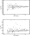 |
Fig. 8 Distributions of λNET and λEFF calculated using different simulation times with a proton energy spectrum at solar minimum (ϕ = 200 MV/c). |
Monte Carlo estimates of λNET and λEFF for the different species of the GCR particles for ϕ = 200 MV/c (solar minimum) and ϕ = 1200 MV/c (solar maximum) conditions.
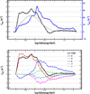 |
Fig. 9 Top panel: comparison of the contribution to the total λNET and total λEFF for a primary proton flux (ϕ = 200 MV/c) and particles of different energies. The dashed line represents the input proton spectrum and is not to scale. Bottom panel: breakdown of the |

Monte Carlo estimates of λNET and λEFF for proton fluxes during a non-recurrent FD and two SEP events.
 |
Fig. 10 Comparison of charging time series for proton (a) and iron nuclei (b) fluxes at ϕ = 200 MV/c. Panel (c) shows a comparison between the charging histograms of the two time series normalized to the number of events. |
5 Discussion of the results
The results for the charge rate λNET from the protons in Table 6 appear to agree relatively well with those presented by Armano et al. (2023), who obtained their results for LPF with a Monte Carlo simulation using GEANT4 version 10.3 (without the DNA module), where the ionization was treated using Opt4 physics and the LEE production from electrons and hadrons was managed with a yield-based approach. Armano et al. (2023) calculated the net charging for the LPF TM on the basis of the INTEGRAL mission measurements by considering the minimum of solar cycle 23 and the maximum of solar cycle 24. The estimates for λNET range from +8 s−1 to +40 s−1, whereas we found +4 s−1 to +51 s−1 under extreme conditions of solar maximum and solar minimum (see Table 6). Wass et al. (2023) estimated a λNET = 29.3 s−1 and a λEFF = 390 s−1 for the proton flux in June 2017. In the same solar modulation condition, the proton flux simulated with our toolkit returns a result of λNET = 31.0 ± 1.0 s−1 and λEFF = 375 ± 14 s−1 with an exceptional agreement despite the different spacecraft geometries considered in the simulations.
When data are compared with Monte Carlo simulations, however, it must be taken into account that the measured charging depends on the TM potential that affects the trajectories of LEE in the gap between the TM and the EH. We recall that in LPF, the charge rate of the two TM was measured in July 2017 to vary from 50–60 s−1 for VTM = –1 V to zero (TM equilibrium potential) for VTM ≈ 1 V, (Wass et al. 2023; Armano et al. 2023). We note that this was one of the main arguments in favor of the presence of LEE in the gap between the TM and the EH and for including the physics of the LEE in the new versions of the Monte Carlo. For this reason, we built an electrostatic finite-element model (FEM) of the GRS in COMSOL.
This multiphysics software is able to propagate the LEE that are produced by the galactic cosmic-ray flux, in the gap between the TM and the EH and to calculate the TM charge rate as a function of the TM potential. The FEM, created upon the CAD of the LPF GRS, reproduces the electrostatic configuration of the TM and the EH. It allowed us to control the voltages of the TM and of the electrodes and to calculate the net flow of electrons that enter and escape from the TM. For the FEM propagation, we considered the electron population on the surfaces of the TM and of the EH generated by the Monte Carlo simulation. The result of the simulation is shown in Figure 13, where we added the contribution of the LEE flows computed with the FEM to the TM charging computed by the Monte Carlo simulation. The TM equilibrium potential here is consistent with the values observed in LPF and calculated in simulations (Wass et al. 2023; Armano et al. 2023). The slightly lower value of the charging predicted in Figure 13, 40 s−1 with respect to 50 s−1, as observed in figure 4 in Armano et al. (2023), is compatible with a lower proton flux.
Our Monte Carlo simulation toolkit still needs improvements, however. The comparison of the results reported in Tables 6, 7, and 8 shows that while the net charging results are similar for the GEANT4 and FLUKA-LEI calculations, the effective charging in FLUKA-LEI appears to be higher by a factor of 2 on average and to agree better with the observations gathered on board LPF (Armano et al. 2017; Grimani et al. 2022). We stress that this discrepancy is much more evident with GCRs than for SEPs because the production of secondary electrons is more relevant (see Grimani et al. 2022, and Fig. 7).
We investigated the possible origin of the discrepancies between FLUKA-LEI and TMCTK. Part of the difference in the results might be due to the spacecraft geometry (FLUKA-LEI uses a realistic reproduction of the LPF geometry). Nevertheless, as stated before, we studied the dependence of the TMCTK results on the material distribution around the TM. We changed the shell material amount and/or their radius, but found no relevant differences.
The main difference between FLUKA-LEI and GEANT4-DNA is attributed to a much larger number of secondary electrons surrounding the test masses in FLUKA-LEI. We stressed in the Introduction that the hadron ionization in GEANT4 presents a sharp cutoff at the average ionization potential in gold of 790 eV, while in FLUKA-LEI, the implementation is carried out down to 10 eV. Moreover, a simple experiment was carried out to compare the performance of the two tools with primary electrons. We simulated a beam of 10 keV electrons crossing a 100 nm thick gold slab. In Figure 14 we compare the spectrum of secondary electrons per incident particle transmitted by the target. The spectrum associated with the GEANT4-DNA simulation exhibits a marked excess at a few eV and appears approximately one order of magnitude below the LEI outcome, in particular below 1 keV. Moreover, the GEANT4-DNA spectrum exhibits sharp step-like variations, typical of discontinuous parameterizations of cross-sections and/or electron mean free path in the 10–100 eV energy interval. This issue was discussed with scientists of the GEANT-4 collaboration. Improvements for low-energy electromagnetic physics in gold are expected in a future release of the DNA module (private communication).
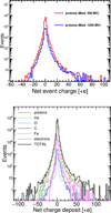 |
Fig. 11 Top panel: Comparison of charging histograms obtained from simulations of proton fluxes at extreme solar minimum (ϕ = 200 MV/c) and solar maximum (ϕ = 1200 MV/c) conditions. Bottom panel: Total charging histogram obtained from complete simulation of CR flux (10 000 seconds) at solar minimum condition (ϕ=200 MV/c), broken down in its contributions from every simulated CR species. |
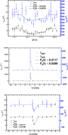 |
Fig. 12 Top panel: Net (black points) and effective (blue points) charging of the LISA TM during the recurrent GCR variation associated with the passage of one high-speed solar wind stream observed with LPF in November 2016. Only the proton flux was simulated. As a comparison, the trend of the simulated proton flux Fp(t), integrated in the 0.5–1.5 GV rigidity bin, was superimposed on the λNET and λEFF data through multiplication by a constant (dashed lines). Central panel: Net (black points) and effective (blue points) charging of the LISA TM during the SEP event of December 13, 2006. The dashed lines show the same comparison as in the top panel with the normalized proton flux. Bottom panel: Net (black points) and effective (blue points) charging of the LISA TM during the Forbush decrease following the SEP event of December 13, 2006 (SEPs were subtracted from the data). The dashed lines show the same comparison as in the top panel with the normalized proton flux. |
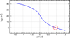 |
Fig. 13 Simulation of the TM net charging evolution as a function of the TM to EH ground electric potential for a proton flux corresponding to the initial operation time frame of LPF. The red point represents the value of electric potential corresponding to zero net charging (equilibrium potential). |
FLUKA-LEI Monte Carlo estimates of λΝΕΤ and λEFF for different species of GCR particles.
6 Impact on the sensitivity of LISA
In the previous sections, we discussed the LISA TM charging through the action of particle fluxes of galactic and solar origin. We now analyze the impact of the charging process on the LISA mission performance. The LISA TM is subjected to a Coulomb force by the interaction of the TM charge with any nonzero average electrostatic field, from nonuniform surface patch potentials (Antonucci et al. 2012b) and/or any applied fields. The formula for the force per unit mass along the LISA sensitive axis, fx, is
 (6)
(6)
where MTM ≈ 2 kg, and QTM are the TM mass and deposited charge. The electric field x-component Ex is expressed in terms of the x-electrode derivative  pF/m, the TM self-capacitance CTOT ≈ 34 pF, and the DC bias voltage Δx, which normalizes the stray electrostatic field component along the x-axis to an electrostatic potential applied to a single x-face GRS electrode (Antonucci et al. 2011; Antonucci et al. 2012b; Brandt & Fichter 2009). A DC bias of about 100 mV has been observed in LISA-like GRS, such as that in the torsion pendulum testbed at the University of Trento and those flown in LPF, and it was electrostatically compensated to a level of Δx = 5 mV in the laboratory and during LPF flight operations (Antonucci et al. 2012b; Armano et al. 2017). We assumed Δx = 5 mV, which is the expected value during LISA science operations following compensation.
A charge event occurring due to short-term GCR flux variations or SEPs causes QTM to change with time and produces a force signal. The time shape of the force is entangled with the time characteristics and with the energy content of the charge event. We described in Section 4 that we are able to reconstruct the evolution of the charging signal (see, e.g., Figure 8) by using Monte Carlo simulations of the different temporal phases of the event. Based on this, the force time-series can be calculated according to Eq. (6).
Figures 15 and 16 show the evolution of the induced force on the LISA test masses for the event on December, 13–15 2006, including SEP and FD. The dynamics of the Forbush decrease was reconstructed as described in Sect. 3 and shown in Figure 6. The flare associated with the December 13, 2006, SEP event was observed at 02:14 UT from NOAA active region 10930. A coronal mass ejection that accelerated protons that were observed with PAMELA between 03:18 UT and 03:49 UT was detected by LASCO C2 at 02:54 and thus revealed a very good magnetic connection between the active region and the PAMELA satellite. The time lag between onset, peak, and decay phases of the SEP event were set on the basis of proton-flux measurements carried out with PAMELA (see Figure 7 and Adriani et al. 2011).
For the performance of LISA, it is interesting to calculate the signal-to-noise ratio (S/N) of the charging events,
 (7)
(7)
with FFT (fx) the Fourier transform of the charge-induced force signal, and  the power spectral density of the residual acceleration on the LISA TMs. We point out that the multiplication of Sɡ by a factor of 4 accounts for the contribution of the four TMs involved in the Michelson interferometer, which expresses the low-frequency limit of the LISA noise sensitivity for the X-Michelson time-delay interferometry (TDI, Tinto & Armstrong 1999; Muratore et al. 2023) combination in terms of the residual force noise on a single TM,
  fm s−2 Hz−1/2 (Armano et al. 2018b; Quang Nam et al. 2023; Colpi et al. 2024). At these frequencies, the observatory sensitivity is completely dominated by TM acceleration noise, and we therefore neglected the noise contribution of interferometry in this calculation (Muratore 2023).
To visualize the effect of the charge signal, we show as an example in Figure 17 the LISA acceleration noise floor Sn along with the charge-induced force signal from the 2006 SEP event. The S/N calculation yielded 0.1 and 20 for the FD and the SEP event, respectively, considering the lowest end of the LISA band, fmin = 20 μΗz in Eq. (7). This indicates that LISA will be able to clearly observe the solar event. Were DC biases Δx 50 mV or larger, Forbush decreases would also pollute the LISA data.
In this calculation, we neglected the effect of the charge-control system in LISA, with the expectation that the response time of a possible continuous discharge will be slow enough, of about 105 seconds, to affect the filtering of the SEP charge dynamics in the LISA band above 10−4 Hz only little. The S/N is probably not much different in the case of a continuous or intermittent discharge.
We recall that about ten SEP events with a particle acceleration above tens of MeV are expected per year, at least for the transfer phase of the LISA satellites and the mission commissioning phase. The rate decreases from 8.5 at the beginning of the science data-taking period to about one at the end of the nominal LISA observation time (Grimani et al. 2025). The ability to distinguish these spurious events with respect to genuine gravitational-wave signals lies in on-board measurements of the satellite radiation monitors (Mazzanti et al. 2023) and in the Monte Carlo simulations to inform the analysis of LISA data (Quang Nam et al. 2023). Additionally, the TM charge might be continuously monitored to allow a possible subtraction of the force disturbance from the observatory TDI time series.
Ultimately, it is worth noting that from Eq. (6), fluctuations on the TM charging process, which we accounted for with the λEFF parameter, would generate force noise on the TM. Although our simulation showed some limit in reproducing LPF measurements, we use the FLUKA-LEI results as shown in Tables 8 and 9 to conclude that under GCR flux, λEFF will not exceed 1500 s−1. This number appears close to what LPF has measured (see Table 1) and would yield, according to Eq. (6), an acceleration noise  fm s−2 Hz−1/2, which is comfortably within the 3 fm s−2 Hz−1/2 allowed in LISA for stray electrostatic forces at 0.1 mHz. This is the lower end of the LISA measurement bandwidth.
In SEP events, together with the net charge λNET, the charge fluctuation λEFF also strongly rises and reaches values up to 6 × 10³ s−1 for medium strong events such as the event on December 13, 2006, or even 6 × 10⁴ s−1 for the strong event on 29 September 1989 (see Tables 7 and 9). For SEP events with longer timescales (3–5 days), the analysis of the impact of such an event in LISA becomes more complicated. In particular, several aspects should be taken into account: the discharge control algorithm that is used, the ability we will have to adjust its parameters in flight, and the equilibrium potential at which the TM would rise. We leave this study for a dedicated paper.
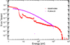 |
Fig. 14 Comparison between the energy spectra of secondary electrons per incident primary electron transmitted by a 150 nm thick gold target simulated using GEANT4-DNA (red curve) and LEI (purple curve). |
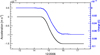 |
Fig. 15 Forbush decrease contribution to the TM accumulated charge (blue line) and to TM acceleration (black line). |
 |
Fig. 16 SEP contribution to the TM accumulated charge (blue line) and to TM acceleration (black line). |
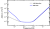 |
Fig. 17 Amplitude spectral density of the LISA force noise and the SEP force signal in a time window of 2 × 10⁵ seconds. |
FLUKA-LEI Monte Carlo estimates of λNET and λEFF for proton fluxes during SEP events.
7 Conclusions
We presented a toolkit for estimating the effects of the space environment on the charging of the LISA TM. The toolkit is based on the GEANT4 package with the GEANT4-DNA module for the generation and propagation of secondary electrons with energies below 100 eV in the outer 150 nm of the gold-plated layers of the TM and EH. Low-energy electrons were found to play a key role in the TM charging based on the comparison of experimental data gathered with LPF and on pre-launch Monte Carlo simulations. The adoption of the DNA module with its more accurate simulation of very LEE returned a better agreement with LPF experimental data, which is in line with other GEANT4 implementations of low-energy electromagnetic physics. A mismatch of about a factor of 2 still remains in the estimate of the charging noise (and thus, of λEFF) with respect to the LPF data. The good agreement between the outcomes of the FLUKA-LEI Monte Carlo and the LPF data suggests that the DNA module describes the role of LEE in the TM charging process still incompletely. This was confirmed by the comparison of FLUKA-LEI and GEANT4-DNA of the energy spectra of simulated electrons emitted from a 100 nm gold layer with incident electron beams of 10 keV energy. This issue was acknowledged by scientists of the GEANT-4 collaboration, and improvements are expected in the future release of the DNA module for low-energy electromagnetic physics in gold. We stress that with respect to the TM net charging (λNET) estimates, GEANT4 and FLUKA-LEI Monte Carlo appear to be consistent with each other and agree well with LPF measurements.
We used the toolkit to consider different case studies associated with the impact of the environment on the LISA mission. In particular, we evaluated the TM charging through GCRs under extreme solar modulation conditions, during recurrent and nonrecurrent short-term variations in the GCR flux, and during SEP events of different intensity. By extrapolating the acceleration noise budget of LPF TM to LISA, the TM charging through GCRs for the extreme cases of solar activity is well below the 3 fm s−2 Hz−1/2 total acceleration noise requirement. LISA will be a signal-dominated mission, and therefore, short-term variations in incident particle fluxes may generate spurious signals that mimic genuine GWs. Whereas GCR recurrent short-term variations with typical durations of 9.1 days are completely off the LISA sensitivity band, the sharp decrease observed during FDs (see Figure 15) generates a step-like signal that would appear in the LISA band. This signal could reach S/N > 1 in the presence of strong stray electrostatic fields, Δx ≥ 50 mV, which are present within the gap of a few millimeters between EH and TM.
Solar energetic particle events were shown to produce increases of several orders of magnitude on the net charging and charge noise over typical timescales from a few hours to five days, depending on the magnetic connection of the spacecraft to an active region on the Sun from which several events are generated in a row. We found that a medium strong event with a duration of a few hours, such as the event measured by PAMELA in December 2006, could generate a strong S/N≈20 signal in the LISA band, which might require the relevant portions of the data stream to be removed.
In addition to spurious signal generation, SEP events with longer timescales may charge the TM to potentials of the order of 1 V, which would affect the mission operation. For LISA, it will therefore also be important to analyze the response of the charge-management system to these events.
Acknowledgements
The authors thank E. Castelli (NASA) for helpful discussions, suggestions and simulations regarding the impact of the charging signal to the LISA sensitivity. This work was funded under the European Space Agency contract No. 4000133571/20/NL/CRS – Test mass charging and LPF lessons learned. F. Dimiccoli and V. Ferroni were funded by ASI – Agenzia Spaziale Ital-iana – accordo attuativo no. 2024-36-HH.0 dell’ accordo quadro ASI/Università di Trento no. 2017-32-H.0 – Addendum no. 2017-29-H.1-2020 All’Accordo no. 2017-29-H.0.
References
- Adriani, O., Barbarino, G. C., Bazilevskaya, G. A., et al. 2011, ApJ, 742, 102 [NASA ADS] [CrossRef] [Google Scholar]
- Agostinelli, S., Allison, J., Amako, K., et al. 2003, Nucl. Instrum. Meth. A, 506, 250 [CrossRef] [Google Scholar]
- Aguilar, M., Cavasonza, L. A., Ambrosi, G., et al. 2021, Phys. Rev. Lett., 127, 271102 [NASA ADS] [CrossRef] [Google Scholar]
- Allison, J., Amako, K., Apostolakis, J., et al. 2006, IEEE Trans. Nucl. Sci., 53, 270 [Google Scholar]
- Allison, J., Amako, K., Apostolakis, J., et al. 2016, Nucl. Instrum. Meth. A, 835, 186 [CrossRef] [Google Scholar]
- Amaro-Seoane, P., Audley, H., Babak, S., et al. 2017, arXiv e-prints, [arXiv:1702.00786] [Google Scholar]
- Antonucci, F., Armano, M., Audley, H., et al. 2011, CQG, 28, 094001 [NASA ADS] [CrossRef] [Google Scholar]
- Antonucci, F., Armano, M., Audley, H., et al. 2012a, CQG, 29, 124014 [NASA ADS] [CrossRef] [Google Scholar]
- Antonucci, F., Cavalleri, A., Dolesi, R., et al. 2012b, Phys. Rev. Lett., 108, 181101 [Google Scholar]
- Araújo, H., Wass, P., Shaul, D., Rochester, G., & Sumner, T. 2005, Astropart. Phys., 22, 451 [Google Scholar]
- Armano, M., Audley, H., Auger, G., et al. 2017, Phys. Rev. Lett., 118, 171101 [NASA ADS] [CrossRef] [Google Scholar]
- Armano, M., Audley, H., Baird, J., et al. 2018a, Astrophys. J., 854, 113 [Google Scholar]
- Armano, M., Audley, H., Baird, J., et al. 2018b, Phys. Rev. Lett., 120, 061101 [NASA ADS] [CrossRef] [Google Scholar]
- Armano, M., Audley, H., Baird, J., et al. 2019, Astrophys. J., 874, 167 [Google Scholar]
- Armano, M., Audley, H., Baird, J., et al. 2023, Phys. Rev. D, 107, 062007 [Google Scholar]
- Battistoni, G., Boehlen, T., Cerutti, F., et al. 2014, in Joint International Conference on Supercomputing in Nuclear Applications + Monte Carlo, 06005 [Google Scholar]
- Bernal, M. A., Bordage, M. C., Brown, J. M. C., et al. 2015, Physica Medica, 31, 861 [Google Scholar]
- Böhlen, T. T., Cerutti, F., Chin, M. P. W., et al. 2014, Nucl. Data Sheets, 120, 211 [CrossRef] [Google Scholar]
- Brandt, N., & Fichter, W. 2009, J. Phys.: Conf. Ser., 154, 012008 [Google Scholar]
- Burger, R. A., Potgieter, M. S., & Heber, B. 2000, J. Geophys. Res.: Space Phys., 105, 27447 [NASA ADS] [CrossRef] [Google Scholar]
- Colpi, M., Danzmann, K., Hewitson, M., et al. 2024, arXiv e-prints, [arXiv:2402.07571] [Google Scholar]
- Cucinotta, F. A., Katz, R., Wilson, J. W., & Dubey, R. R. 1996, in American Institute of Physics Conference Series, 362, Two-Center Effects in Ion-atom Collisions: A Symposium in honor of M. Eugene Rudd, 245 [Google Scholar]
- Forbush, S. E. 1937, Phys. Rev., 51, 1108 [NASA ADS] [CrossRef] [Google Scholar]
- Forbush, S. E. 1954, J. Geophys. Res., 59, 525 [Google Scholar]
- Forbush, S. E. 1958, J. Geophys. Res., 63, 651 [CrossRef] [Google Scholar]
- Furman, M. A., & Pivi, M. T. F. 2002, Phys. Rev. ST Accel. Beams, 5, 124404 [Google Scholar]
- García Marirrodriga, C., Pacros, A., Strandmoe, S., et al. 2021, A&A, 646, A121 [CrossRef] [EDP Sciences] [Google Scholar]
- Geant4 Collaboration 2024, Geant4 Physics Reference Manual, https://geant4-userdoc.web.cern.ch/UsersGuides/PhysicsReference-Manual/html/index.html [Google Scholar]
- Gleeson, L. J., & Axford, W. I. 1968, ApJ, 154, 1011 [NASA ADS] [CrossRef] [Google Scholar]
- Grimani, C. 2004, A&A, 418, 649 [NASA ADS] [CrossRef] [EDP Sciences] [Google Scholar]
- Grimani, C. 2007, A&A, 474, 339 [NASA ADS] [CrossRef] [EDP Sciences] [Google Scholar]
- Grimani, C., Fabi, M., Finetti, N., & Tombolato, D. 2008, Int. Cosmic Ray Conf., 1, 485 [NASA ADS] [Google Scholar]
- Grimani, C., Fabi, M., Finetti, N., & Tombolato, D. 2009, Class. Quant. Grav., 26, 215004 [NASA ADS] [CrossRef] [Google Scholar]
- Grimani, C., Fabi, M., Finetti, N., Laurenza, M., & Storini, M. 2013, in Journal of Physics Conference Series, 409, 012159 [Google Scholar]
- Grimani, C., Fabi, M., Lobo, A., Mateos, I., & Telloni, D. 2015, CQG, 32, 035001 [NASA ADS] [CrossRef] [Google Scholar]
- Grimani, C., Cesarini, A., Fabi, M., et al. 2020a, ApJ, 904, 64 [NASA ADS] [CrossRef] [Google Scholar]
- Grimani, C., Cesarini, A., Fabi, M., & Villani, M. 2020b, Class. Quant. Grav., 38, 045013 [Google Scholar]
- Grimani, C., Andretta, V., Chioetto, P., et al. 2021, A&A, 656, A15 [NASA ADS] [CrossRef] [EDP Sciences] [Google Scholar]
- Grimani, C., Villani, M., Fabi, M., Cesarini, A., & Sabbatini, F. 2022, A&A, 666, A38 [NASA ADS] [CrossRef] [EDP Sciences] [Google Scholar]
- Grimani, C., Andretta, V., Antonucci, E., et al. 2023a, A&A, 677, A45 [NASA ADS] [CrossRef] [EDP Sciences] [Google Scholar]
- Grimani, C., Fabi, M., Sabbatini, F., et al. 2023b, Astrophys. Space Sci., 368, 78 [CrossRef] [Google Scholar]
- Grimani, C., Villani, M., Fabi, M., & Sabbatini, F. 2024, J. High Energy Astrophys., 42, 38 [Google Scholar]
- Grimani, C., Fabi, M., Sabbatini, F., & Villani, M. 2025, Class. Quant. Grav., 42, 095009 [Google Scholar]
- Incerti, S., Baldacchino, G., Bernal, M., et al. 2010a, Int. J. Model. Simul. Sci. Comput., 01, 157 [Google Scholar]
- Incerti, S., Ivanchenko, A., Karamitros, M., et al. 2010b, Med. Phys., 37, 4692 [CrossRef] [Google Scholar]
- Incerti, S., Kyriakou, I., Bernal, M. A., et al. 2018, Med. Phys., 45, e722 [CrossRef] [Google Scholar]
- Ivanchenko, V., Incerti, S., Allison, J., et al. 2014, in Geant4 Electromagnetic Physics: Improving Simulation Performance and Accuracy, 03101 [Google Scholar]
- Mazzanti, D., Guberman, D., Aran, A., et al. 2023, PoS, ICRC2023, 1494 [Google Scholar]
- Miroshnichenko, L. I., De Koning, C. A., & Perez-Enriquez, R. 2000, Space Sci. Rev., 91, 615 [Google Scholar]
- Moskalenko, I. V., & Strong, A. W. 1998, ApJ, 493, 694 [NASA ADS] [CrossRef] [Google Scholar]
- Müller, D., Cyr, O. C. St., Zouganelis, I., et al. 2020, A&A, 642, A1 [NASA ADS] [CrossRef] [EDP Sciences] [Google Scholar]
- Muratore, M. 2023, PRD, 108, 082004 [Google Scholar]
- Muratore, M., Hartwig, O., Vetrugno, D., Vitale, S., & Weber, W. J. 2023, Phys. Rev. D, 107, 082004 [Google Scholar]
- Papini, P., Grimani, C., & Stephens, S. 1996, Nuovo Cim., C19, 367 [NASA ADS] [CrossRef] [Google Scholar]
- Quang Nam, D., Martino, J., Lemière, Y., et al. 2023, Phys. Rev. D, 108, 082004 [Google Scholar]
- Reames, D. V. 2021, Solar Energetic Particles. A Modern Primer on Understanding Sources, Acceleration and Propagation, 978 [Google Scholar]
- Reames, D. V. 2022, Front. Astron. Space Sci., 9, 890864 [NASA ADS] [CrossRef] [Google Scholar]
- Rodríguez-Pacheco, J., Wimmer-Schweingruber, R. F., Mason, G. M., et al. 2020, A&A, 642, A7 [Google Scholar]
- Sakata, D., Incerti, S., Bordage, M. C., et al. 2016, J. Appl. Phys., 120, 244901 [CrossRef] [Google Scholar]
- Sakata, D., Kyriakou, I., Okada, S., et al. 2018, Med. Phys., 45, 2230 [Google Scholar]
- Schou, J. 1980, Phys. Rev. B, 22, 2141 [NASA ADS] [CrossRef] [Google Scholar]
- Shaul, D. N. A., Aplin, K. L., Araújo, H., et al. 2006, in American Institute of Physics Conference Series, 873, Laser Interferometer Space Antenna: 6th International LISA Symposium, eds. S. M. Merkovitz & J. C. Livas (AIP), 172 [Google Scholar]
- Shikaze, Y., Haino, S., Abe, K., et al. 2007, Astropart. Phys., 28, 154 [NASA ADS] [CrossRef] [Google Scholar]
- Simpson, J. A. 1983, Annu. Rev. Nucl. Part. Sci., 33, 323 [Google Scholar]
- Singh, A. K., & Bhargawa, A. 2019, Ap&SS, 364, 12 [NASA ADS] [CrossRef] [Google Scholar]
- Taioli, S., Dapor, M., Dimiccoli, F., et al. 2023, Class. Quant. Grav., 40, 075001 [Google Scholar]
- Tinto, M., & Armstrong, J. W. 1999, Phys. Rev. D, 59, 102003 [NASA ADS] [CrossRef] [Google Scholar]
- Tran, H. N., Archer, J., Baldacchino, G., et al. 2024, Med. Phys., 51, 5873 [Google Scholar]
- Usoskin, I. G., Bazilevskaya, G. A., & Kovaltsov, G. A. 2011, J. Geophys. Res.: Space Phys., 116, A02104 [Google Scholar]
- Usoskin, I. G., Gil, A., Kovaltsov, G. A., Mishev, A. L., & Mikhailov, V. V. 2017, J. Geophys. Res.: Space Phys., 122, 3875 [Google Scholar]
- Van Hove, M., Weinberg, W., & Chan, C. 1986, Low-Energy Electron Diffraction: Experiment, Theory and Surface Structure Determination, Springer Series in Surface Sciences (Springer Berlin Heidelberg) [Google Scholar]
- Vidano, S., Novara, C., Pagone, M., & Grzymisch, J. 2022, Acta Astronaut., 193, 731 [Google Scholar]
- Villani, M., Benella, S., Fabi, M., & Grimani, C. 2020, Appl. Surf. Sci., 512, 145734 [NASA ADS] [CrossRef] [Google Scholar]
- Villani, M., Cesarini, A., Fabi, M., & Grimani, C. 2021, CQG, 38, 145005 [NASA ADS] [CrossRef] [Google Scholar]
- Villani, M., Sabbatini, F., Grimani, C., Fabi, M., & Cesarini, A. 2023, Exp. Astron., 56, 1 [Google Scholar]
- Villani, M., Fabi, M., Grimani, C., et al. 2024a, Results Phys., 60, 107638 [Google Scholar]
- Villani, M., Sabbatini, F., Cesarini, A., Fabi, M., & Grimani, C. 2024b, Exp. Astron., 58, 15 [Google Scholar]
- Vlachoudis, V. 2009, in International Conference on Mathematics, Computational Methods & Reactor Physics (M&C 2009), Saratoga Springs, New York, 790 [Google Scholar]
- Vocca, H., Grimani, C., Amico, P., et al. 2004, Class. Quant. Grav., 21, S665 [Google Scholar]
- Wass, P. J., Araújo, H. M., Shaul, D. N. A., & Sumner, T. J. 2005, Class. Quant. Grav., 22, S311 [Google Scholar]
- Wass, P. J., Sumner, T. J., Araújo, H. M., & Hollington, D. 2023, Phys. Rev. D, 107, 022010 [Google Scholar]
See, e.g., https://www.spenvis.oma.be/
Events with zero deposit are not included in the charging histograms.
All Tables
Net and effective TM charging and TM equilibrium potential measured with LPF (Armano et al. 2017, 2023).
Parameterization of electron energy spectra above 20 MeV at solar minimum and solar maximum.
Parameterizations of the proton energy spectra during a recurrent variation in the proton-dominated flux measured with LPF between November 20 and December 4, 2016.
Parameterizations of the proton energy spectra during a Forbush decrease observed on December 14–16, 2006.
Monte Carlo estimates of λNET and λEFF for the different species of the GCR particles for ϕ = 200 MV/c (solar minimum) and ϕ = 1200 MV/c (solar maximum) conditions.
Monte Carlo estimates of λNET and λEFF for proton fluxes during a non-recurrent FD and two SEP events.
FLUKA-LEI Monte Carlo estimates of λΝΕΤ and λEFF for different species of GCR particles.
FLUKA-LEI Monte Carlo estimates of λNET and λEFF for proton fluxes during SEP events.
All Figures
|
Fig. 1 Top panel: LISA spacecraft simplified matter distribution around the TM. Bottom panel: magnified view of the central part of the geometry modeling the GRS and the TM in GEANT4. The 150 nm wide cubic box that models the last interface of the EH and the spherical shielding shells are visualized in wireframe mode for visualization purposes. |
| In the text | |
|
Fig. 2 Low-energy electron yield of the kinetic emission processes for protons (p; red) and α particles (blue) that perpendicularly cross the gold surfaces (Y90) as a function of p and α energy. |
| In the text | |
|
Fig. 3 From top to bottom: Proton (p, red), helium (He, blue), carbon (C, magenta), oxygen (O, green), nitrogen (N, cyan), and iron (Fe, yellow) cosmic-ray energy spectra at solar minimum (ϕ = 200 MV/c; continuous lines) and solar maximum (ϕ = 1200 MV/c; dashed lines) as extreme conditions for LISA. |
| In the text | |
|
Fig. 4 Galactic electron energy spectra at solar minimum (dashed line) and solar maximum (continuous line) for LISA. The interstellar spectrum is represented by the top dotted line (Moskalenko & Strong 1998). |
| In the text | |
|
Fig. 5 Recurrent short-term variations of GCRs observed with LPF between November 21 and December 4, 2016. The continuous lines indicate the decrease phase, and the dashed lines show the recovery phase. The top continuous red line indicates the proton energy spectrum at the onset of the event. |
| In the text | |
|
Fig. 6 Forbush decrease observed on December 14–15, 2006 with the PAMELA experiment in space and on Earth with neutron monitors. |
| In the text | |
|
Fig. 7 Solar energetic proton fluxes observed during the evolution of the gradual events on September 29, 1989 (dashed line), and December 13, 2006 (continuous line). The different phases of the events are indicated. The timings of the events shown in the figure appear in Table 7. |
| In the text | |
|
Fig. 8 Distributions of λNET and λEFF calculated using different simulation times with a proton energy spectrum at solar minimum (ϕ = 200 MV/c). |
| In the text | |
|
Fig. 9 Top panel: comparison of the contribution to the total λNET and total λEFF for a primary proton flux (ϕ = 200 MV/c) and particles of different energies. The dashed line represents the input proton spectrum and is not to scale. Bottom panel: breakdown of the |
| In the text | |
|
Fig. 10 Comparison of charging time series for proton (a) and iron nuclei (b) fluxes at ϕ = 200 MV/c. Panel (c) shows a comparison between the charging histograms of the two time series normalized to the number of events. |
| In the text | |
|
Fig. 11 Top panel: Comparison of charging histograms obtained from simulations of proton fluxes at extreme solar minimum (ϕ = 200 MV/c) and solar maximum (ϕ = 1200 MV/c) conditions. Bottom panel: Total charging histogram obtained from complete simulation of CR flux (10 000 seconds) at solar minimum condition (ϕ=200 MV/c), broken down in its contributions from every simulated CR species. |
| In the text | |
|
Fig. 12 Top panel: Net (black points) and effective (blue points) charging of the LISA TM during the recurrent GCR variation associated with the passage of one high-speed solar wind stream observed with LPF in November 2016. Only the proton flux was simulated. As a comparison, the trend of the simulated proton flux Fp(t), integrated in the 0.5–1.5 GV rigidity bin, was superimposed on the λNET and λEFF data through multiplication by a constant (dashed lines). Central panel: Net (black points) and effective (blue points) charging of the LISA TM during the SEP event of December 13, 2006. The dashed lines show the same comparison as in the top panel with the normalized proton flux. Bottom panel: Net (black points) and effective (blue points) charging of the LISA TM during the Forbush decrease following the SEP event of December 13, 2006 (SEPs were subtracted from the data). The dashed lines show the same comparison as in the top panel with the normalized proton flux. |
| In the text | |
|
Fig. 13 Simulation of the TM net charging evolution as a function of the TM to EH ground electric potential for a proton flux corresponding to the initial operation time frame of LPF. The red point represents the value of electric potential corresponding to zero net charging (equilibrium potential). |
| In the text | |
|
Fig. 14 Comparison between the energy spectra of secondary electrons per incident primary electron transmitted by a 150 nm thick gold target simulated using GEANT4-DNA (red curve) and LEI (purple curve). |
| In the text | |
|
Fig. 15 Forbush decrease contribution to the TM accumulated charge (blue line) and to TM acceleration (black line). |
| In the text | |
|
Fig. 16 SEP contribution to the TM accumulated charge (blue line) and to TM acceleration (black line). |
| In the text | |
|
Fig. 17 Amplitude spectral density of the LISA force noise and the SEP force signal in a time window of 2 × 10⁵ seconds. |
| In the text | |
Current usage metrics show cumulative count of Article Views (full-text article views including HTML views, PDF and ePub downloads, according to the available data) and Abstracts Views on Vision4Press platform.
Data correspond to usage on the plateform after 2015. The current usage metrics is available 48-96 hours after online publication and is updated daily on week days.
Initial download of the metrics may take a while.