| Issue |
A&A
Volume 700, August 2025
|
|
|---|---|---|
| Article Number | A76 | |
| Number of page(s) | 11 | |
| Section | Extragalactic astronomy | |
| DOI | https://doi.org/10.1051/0004-6361/202453110 | |
| Published online | 05 August 2025 | |
Traces of the evolution of cosmic void galaxies: An integral field spectroscopy-based analysis
1
Instituto de Astronomía teórica y experimental-Conicet, Laprida 854, Córdoba, Argentina
2
Observatorio Astronómico de Córdoba, Universidad Nacional de Córdoba, Laprida 854, X5000BGR Córdoba, Argentina
3
Consejo de Investigaciones Científicas y Técnicas de la República Argentina, Buenos Aires, Argentina
⋆ Corresponding author: This email address is being protected from spambots. You need JavaScript enabled to view it.
Received:
21
November
2024
Accepted:
12
June
2025
Abstract
Context. Galaxies in the most underdense regions of the Universe, known as cosmic voids, exhibit astrophysical properties that suggest a distinct evolutionary path compared to galaxies in denser environments. Numerical simulations indicate that the assembly of void galaxies occurs later, leading to galaxies with younger stellar populations, low metallicities, and high gas content in their halos, which provides the fuel to sustain elevated star formation activity.
Aims. Our objective in this work is to test these numerical predictions using observational data by comparing galaxies in voids with galaxies in non-void environments.
Methods. We used voids identified in the SDSS data and selected galaxies from the MaNGA survey, which offers integral field spectroscopy (IFS) for each galaxy. This IFS data allows for state-of-the-art modeling of their stellar populations. We separated the galaxies into void and non-void samples, mimicked the magnitude distribution, and compared their integrated astrophysical properties, as well as the metallicity and age profiles, through a stacking technique. We analyzed early-type galaxies (ETGs) and late-type galaxies (LTGs) separately.
Results. We find that void galaxies tend to host younger and less metal-rich stellar populations. This trend is observed both as a function of mass and in samples with matched magnitude distributions. With respect to the gas mass, we do not find differences across environments. When dividing galaxies into ETGs and LTGs, we observe that ETGs show negative gradients in both age and metallicity, with void galaxies consistently appearing younger and less metal-rich. For LTGs, age gradients are also negative, indicating younger populations in void galaxies. However, we do not find statistically significant differences in the stellar metallicity gradients between void and non-void environments.
Conclusions. Our results show how the astrophysical properties of galaxies in voids differ from those of galaxies in the rest of the Universe. This suggests that the void environment plays a role in the evolution of its galaxies, delaying their assembly and growth.
Key words: galaxies: evolution / galaxies: statistics / large-scale structure of Universe
© The Authors 2025
 Open Access article, published by EDP Sciences, under the terms of the Creative Commons Attribution License (https://creativecommons.org/licenses/by/4.0), which permits unrestricted use, distribution, and reproduction in any medium, provided the original work is properly cited.
This article is published in open access under the Subscribe to Open model. This email address is being protected from spambots. You need JavaScript enabled to view it. to support open access publication.
1. Introduction
Galaxy evolution is driven by both in situ processes and environmental effects. The large-scale and local densities of the galactic environment influence the astrophysical properties of galaxies. In this context, the most underdense regions of the Universe, known as cosmic voids, are particularly interesting for studying galaxies. In these regions, galaxies evolve in an environment that can be free from interactions between them. As a result, these galaxies may have populations more representative of in situ processes (van de Weygaert & Platen 2011; Kreckel et al. 2011).
Other authors have previously studied galaxies in voids using observational data. In general, studies show that these environments, in contrast to galaxies in denser regions, host a population of bluer galaxies (Rojas et al. 2004; von Benda-Beckmann & Müller 2008; Hoyle et al. 2012), with higher star formation rates (SFRs; Rojas et al. 2005; Ceccarelli et al. 2008; Moorman et al. 2016, and typically of late-type morphology (Hoyle et al. 2005; Porter et al. 2023; Argudo-Fernández et al. 2024). All of these properties are consistent with the idea of delayed evolution for galaxies in such environments. Domínguez-Gómez et al. (2023a) use a sample of spectra from galaxies in voids and denser environments to reconstruct the star formation histories of these galaxies, revealing that those in voids exhibit delayed star formation histories compared to other samples.
Another approach to studying the influence of the environment is through numerical simulations. Modern simulations generally produce a population of void galaxies with properties qualitatively comparable to those in observational data (Rosas-Guevara et al. 2022; Curtis et al. 2024). One advantage of numerical simulations is their ability to trace the assembly history of galaxies through merger trees. These studies also confirm a delayed evolution for galaxies in voids compared to those in denser environments (Martizzi et al. 2020; Alfaro et al. 2020; Rodríguez Medrano et al. 2022; Rodríguez-Medrano et al. 2024).
Differences in galaxy assembly translate into variations in the ages of their stellar populations, which can be reflected in their metallicities. In Rodríguez-Medrano et al. (2024), using the IllustrisTNG simulation (Nelson et al. 2019; Pillepich et al. 2018; Springel et al. 2018), we find lower stellar metallicities, at a given galaxy mass, for galaxies in voids compared to the general population. This is consistent with results from observational data (Domínguez-Gómez et al. 2023b) based on a sample of galaxies from the Sloan Digital Sky Survey Data Release 7 (SDSS-DR7) (Abazajian et al. 2009), with optical spectra integrated over the central regions of each galaxy (3 arcsec aperture).
Another feature detected in void environments is a lower stellar-to-halo mass relation (SHMR) for the galaxies (Habouzit et al. 2020; Rosas-Guevara et al. 2022). At a given stellar mass, void galaxies tend to have larger dark matter halos, which can retain more gas (Rodríguez-Medrano et al. 2024). As shown in Scholz-Díaz et al. (2023), halo mass influences the star formation history of galaxies. Galaxies with younger stellar populations inhabit halos with a lower stellar-to-halo mass ratio (Scholz-Díaz et al. 2022). These predictions of the SHMR in numerical simulations have also been explored in observational data. Douglass et al. (2019), investigate the SHMR in void galaxies and find no significant difference between the halo masses in void and non-void environments. We also study this relation in Rodríguez-Medrano et al. (2023) using SDSS galaxies with halo masses obtained through the method of Rodriguez & Merchán (2020) but do not obtain conclusive results. With regard to gas content, (Florez et al. 2021) detects an excess of gas in void galaxies. Therefore, the question of halo mass, and particularly the gas content of galaxies in voids, remains an open topic.
Integral field spectroscopy (IFS) is an observational technique that captures spectral information across a two-dimensional (2D) field of view. This provides two spatial dimensions plus an additional spectral dimension, forming what is known as a datacube. The IFS technique has proven highly effective for studying the stellar composition of galaxies with spatial resolution, capturing variations in stellar populations and other properties across galactic structures (Bacon et al. 2001; Sánchez et al. 2012; Croom et al. 2012). This technique is used, for example, in the CAVITY project (Calar Alto Void Integral-field Treasury surveY) (Pérez et al. 2024) to study galaxies in voids. The sample of void galaxies from this project exhibits a lower stellar mass surface density, younger ages, and higher specific SFRs (Sánchez et al. 2024). These differences in the properties of void galaxies are present in all morphological types (Conrado et al. 2024).
The Mapping Nearby Galaxies at APO (MaNGA) survey, part of the SDSS-IV project, is currently the largest IFS survey (Bundy et al. 2015). The MaNGA survey has observed approximately 10 000 galaxies in the local Universe (z < 0.15). These data have been used to apply methods such as the “fossil record method”, which leverages spatial resolution to apply spectral energy distribution (SED) models and deduce the star formation histories (SFH) and chemical enrichment histories (ChEH) of galaxies (Ibarra-Medel et al. 2016; Sánchez et al. 2022; Riffel et al. 2023). This extensive sample enables studies of the relationship between a galaxy’s evolution and its cosmic environment, particularly in cosmic voids. Since MaNGA galaxies are part of the original SDSS sample (York et al. 2000), we can assign MaNGA galaxies to voids identified in a complete volume-limited sample from the SDSS. This allows us to compare galaxies in voids with those in denser environments and to investigate evolutionary differences and astrophysical properties based on the environment, thereby mapping the impact of large-scale structures on galaxies.
This paper is organized as follows. In Section 2, we describe the data used in this work, including the galaxy sample and the void catalog. In Section 3, we present our results, dividing the section into parts that examine the integrated properties of galaxies, the results related to galaxy morphologies, and the galaxy gradients. In Section 4, we discuss the implications of our analysis, and in Section 5, we summarize the main conclusions of this study.
2. Data
The MaNGA (Bundy et al. 2015) and SDSS (Bacon et al. 2001) surveys cover the same spatial region, ensuring a substantial overlap that enables the effective integration of data from both sources. This overlap is advantageous as it enables the use of voids identified within SDSS, which provides a dense sample of galaxies suitable for the robust identification of underdense regions in the Universe. We subsequently studied galaxies from the MaNGA survey, utilizing its IFS capabilities, which are particularly beneficial for efficiently modeling stellar populations and their properties. Integral field spectroscopy (IFS) offers comprehensive spatial coverage by capturing spectral information across a 2D field, allowing detailed analysis of various stellar properties at different locations within galaxies. This spatially resolved spectroscopy makes it possible to examine gradients and variations in key stellar attributes, providing a more holistic view of galactic evolution. The MaNGA survey is designed to obtain the IFS of nearby galaxies, and its main sample is divided into two subsamples: the Primary Sample (PS) and the Secondary Sample (SS). These subsamples are optimized to cover different regions of galaxies. The PS includes galaxies with coverage extending to at least 1.5 Re (effective radius), enabling detailed studies of their inner regions, while the SS extends this coverage to at least 2.5 Re, facilitating the analysis of their outer parts, such as stellar halos and large-scale dynamics.
As described in Yan et al. (2016) and Wake et al. (2017), this difference in spatial coverage means that the SS consists of galaxies observed at higher redshifts compared to the PS. This is because observing more distant galaxies is necessary to cover a larger area with the same integral field unit (IFU) size.
For the PS, the median signal-to-noise ratio (S/N) per fiber in the outer regions at 1.5 Re is 8.3, increasing to 37.3 in an elliptical annulus after stacking the fibers. For the Secondary Sample, the median S/N per fiber in the outer regions (at 2.5 Re) is 2.3, increasing to 11.4 in an elliptical annulus after stacking.
By leveraging the overlap between SDSS and MaNGA, this study aims to shed light on the evolutionary differences that arise from environmental variations within large cosmic structures.
2.1. MaNGA: Average properties and morphology
In this work, we used the data products extracted from the datacubes with the pyPipe3D pipeline, applied to the MaNGA data from SDSS-DR17 (Sánchez et al. 2016a,b, 2022; Lacerda et al. 2022). This analysis includes both integrated and spatially resolved properties of the stellar population and the ionized gas. The pyPipe3D code employs a binning method based on continuum segmentation to enhance the S/N while preserving the spatial structure of galaxies. Our analysis utilizes the MASTAR_SLOG stellar library (Yan et al. 2019), which includes simple stellar populations (SSPs) with 39 ages and seven metallicities, along with a Salpeter initial mass function (IMF). Additionally, it incorporates kinematic parameters such as stellar velocity and velocity dispersion, treated as free parameters, while accounting for interstellar dust extinction effects.
In this work, we selected only galaxies with high S/N, excluding merging systems, galaxies with uncertain redshift determinations, or those contaminated by a bright star in the field of view. These selection criteria are indicated by the QCFLAG of the catalog used.
We used the second version of the morphological classification obtained by Vázquez-Mata et al. (2022) from the visual classification of MaNGA galaxies in the SDSS-DR17, using mosaics generated by combining r-band images from the SDSS and the DESI Legacy Survey (Dey et al. 2019).
2.2. MaNGA: Stellar profiles
To analyze the radial behavior of certain properties in our sample, we used radial profiles constructed from the publicly available MEGACUBES dataset1 (Riffel et al. 2023). These datacubes provide maps of various properties and emission-line profiles for each spaxel, along with a table of average properties over different galaxy radii. For the stellar populations, measurements have been made using full spectral fitting for stellar population synthesis on the datacubes, using the STARLIGHT code (Cid Fernandes et al. 2005; Cid Fernandes 2018). In addition, these MEGACUBES contain absorption-free emission line datacubes. Emission line fitting was performed using the IFSCUBE3 Python package Ruschel-Dutra & Dall’Agnol De Oliveira (2020), Ruschel-Dutra et al. (2021) to fit the profiles of the most prominent optical emission lines.
The analysis employed a binning method that enhanced the S/N while preserving spatial resolution. The stellar libraries used are based on updated MILES models (González Delgado et al. 2005; Vazdekis et al. 2010, 2016), covering a range of 21 ages and four metallicities. Additionally, a Salpeter initial mass function is adopted. The fits included kinematic parameters, such as stellar velocity and velocity dispersion, which were incorporated as key elements in the spectral modeling.
The profiles provided by MEGACUBES extend to at least 1.5 Re or 2 Re, depending on whether the galaxies belong to the Primary or Secondary sample, respectively. The catalog presents metallicity and age profiles for each galaxy, computed by averaging the spaxels that fall within specific radial intervals, expressed in units of the effective radius (Re).
2.3. Void and non-void galaxies
We used the void finder algorithm described in Ruiz et al. (2015, 2019) to identify spherical voids in a sample of galaxies of the SDSS-DR12 catalog Alam et al. (2015). Voids were identified by finding spheres in a galaxy distribution with integrated contrast density (Δ) below some threshold; in our case, we used Δ < −0.9. The radius of the void (rvoid) is defined by the distance from the center of the sphere, at which Δ = −0.9 is reached. The tracer galaxies selected are at z > 0.03, have an absolute magnitude in r-band Mr < −20.19 and constitute a completed volume sample at z < 0.12. We assumed a cosmology with ΩM = 0.31 and ΩΛ = 0.69. We selected all voids with rvoid > 12 h−1 Mpc to avoid spurious voids due to shot noise.
For this selection of voids, we computed the distance from each galaxy in the MaNGA sample to the nearest spherical void center, normalizing the distances by the void radius. Galaxies with a distance d < rvoid were classified as void galaxies, while those with d > rvoid were categorized as non-void galaxies. Galaxies whose nearest void was close to the catalog edges were excluded from the analysis, specifically those at a distance of d < 1.5 rvoid from the edge. This selection left us with 176 void galaxies and 3191 non-void galaxies. We include in Appendix A the distributions of redshift, effective radius, and inclination angle of the galaxies in each sample to better characterize them.
3. Results
In this section, we present the results of our analysis. We focus on the stellar metallicity, age, and gas content of galaxies, while also examining general properties such as colors and SFRs. Our goal is to compare them with the predictions made in Rodríguez-Medrano et al. (2024), who found that void galaxies have a higher gas mass, lower stellar metallicity, and younger stellar populations compared to non-void galaxies.
3.1. General properties
As mentioned in the introduction, several studies have established that void galaxies exhibit bluer colors and higher SFRs compared to galaxies in denser environments. Part of this effect is due to the fact that the magnitude distribution of void galaxies is typically biased toward fainter galaxies, as shown in Figure 1. The gray histogram corresponds to the r-band absolute magnitude distribution of non-void galaxies, while the red distribution represents the void sample. A clear difference in the magnitude distribution between the two samples is evident. Since fainter galaxies are typically bluer, more star-forming, and younger, it is important, when comparing void and non-void galaxies, to study the galaxies as a function of magnitude or to create matched samples by replicating the magnitude distribution to avoid potential biases.
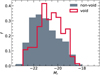 |
Fig. 1. Distribution of r-band absolute magnitudes for the galaxy samples. The filled gray histogram represents the non-void galaxy sample, while the red histogram shows the distribution for the void-galaxysample. |
We first analyzed the colors and SFRs of galaxies in our sample, as calculated from MaNGA data (Sánchez et al. 2022).
We then extended the analysis to focus on the key properties relevant to this study: stellar metallicity, stellar age, and the gas content of the galaxies.
In Fig. 2, we present the color and SFR for our MaNGA dataset. The top panel shows the mean g − r color as a function of the absolute magnitude in the r-band. The solid gray line indicates the results for the non-void galaxy sample, while the dashed red line represents the void galaxy sample. The shaded regions around each line indicate the uncertainty in the mean, calculated as  (where s is the standard deviation and n is the sample size). The trend reveals consistently lower g − r values in all magnitude bins for void galaxies, with some differences exceeding the error bars. This suggests that void galaxies are systematically bluer. In the bottom panel, we show the SFR. The SFR is calculated from the luminosity of the Hα emission line, which is corrected for extinction caused by interstellar dust and converted into SFR using an empirical relation Kennicutt (1998). The figure shows a tendency for galaxies in voids to exhibit higher mean SFR values than galaxies in non-voids.
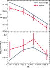 |
Fig. 2. Astrophysical properties of galaxies as a function of r-band absolute magnitude for void and non-void galaxies. Top panel: g − r color. Bottom panel: Star formation rate (SFR). Both panels show the relation for non-void galaxies (solid gray line) and void galaxies (dashed red line). Error bars indicate the uncertainty associated with the mean value. |
Fig. 3 shows various properties of the galaxies as a function of the absolute r-band magnitude. In all panels, the dashed red line corresponds to void galaxies, while the solid gray line corresponds to non-void galaxies. For intensive properties such as stellar age and metallicity, we use the value at the effective radius (Re), derived from the azimuthally averaged radial profiles. These profiles are constructed using elliptical annuli up to the maximum radius covered by the field of view (FoV) (Sánchez et al. 2022). The value at Re is taken as a representative proxy for the galaxy-wide average, as supported by previous studies (Moustakas et al. 2010; Sánchez et al. 2016b). This approach mitigates biases due to varying spatial coverage among galaxies in the sample.
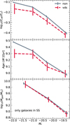 |
Fig. 3. Astrophysical properties of galaxies as a function of r-band absolute magnitude. Top panel: Luminosity weighted stellar metallicity. Middle panel: Luminosity weighted galaxy age. Bottom panel: Gas mass for galaxies in the SS. The solid gray line represents the relation for the non-void galaxy sample, while the dashed red line represents the relation for the void galaxy sample. Error bars indicate the uncertainty associated with the mean value. |
The top panel displays the luminosity-weighted stellar metallicity at the effective radius Re. Across the entire range of magnitudes analyzed, void galaxies are systematically less metal-rich than non-void galaxies. These differences have a statistical significance of approximately ∼1σ, where σ is the error in the mean. The middle panel shows the luminosity-weighted age. For the faintest magnitude bin, there is no statistically significant difference between void and non-void galaxies. However, for the remaining bins, the void galaxy sample consistently shows lower average ages than the non-void sample. The bottom panel presents the mean gas mass. Dust extinction serves as an indicator of the molecular gas content through its connection with the dust-to-gas ratio (Brinchmann et al. 2004). The gas mass is estimated by integrating the molecular gas surface density (Σmol) across the FoV of each IFU, where Σmol is derived from the spaxel-by-spaxel AV, gas parameter using the linear calibrator from Barrera-Ballesteros et al. (2021). Given that the gas content is estimated by summing the contributions across the entire FoV, galaxies in the PS, having a smaller FoV, may be biased toward a lower gas content compared to galaxies in the SS, which have a larger FoV. For this reason, we present gas estimates only for the SS. The relation was calculated using only 79 galaxies in voids (1193 for non-void), which led us to divide the sample into three equal-number bins to increase the number of galaxies per bin. In this case, Fig. 3 shows that the estimated mean gas content in galaxies does not differ with environment.
3.2. Morphology
It is well established that galaxy morphology is closely related to other galactic properties and that the environment plays a significant role in shaping galaxy morphology. We separated galaxies into early- and late-type categories to analyze the differences between galaxies in void and non-void environments across different morphological types.
We used the visual classification from Vázquez-Mata et al. (2022). This classification is based on image mosaics combining r-band images from the SDSS and the DESI Legacy Surveys, identifying 13 Hubble types. Each galaxy is assigned a numerical code (T-type) of −5, −2, or a value between 0 and 10, corresponding to its most probable morphological type (E, S0, S0a, Sa, Sab, Sb, Sbc, Sc, Scd, Sd, Sdm, Sm, and Irr). Since we do not have a sufficiently large number of void galaxies to analyze each type individually, we generalized the sample by dividing it into early-type galaxies (ETGs; T − type ≤ 0) and late-type galaxies (LTGs; T − type ≥ 1). We did not consider T − type = 10, which corresponds to irregular galaxies.
In Fig. 4, we present the results of this classification. The left bars show the proportions of galaxies classified as early types, while the right bars represent late-type galaxies. Void galaxies are shown in red, and non-void galaxies are indicated with dashed gray bars. The error bars represent the 95% confidence intervals for each proportion. We find that in our sample of galaxies, ∼35% (∼65%) of void galaxies are ETGs (LTGs), compared to ∼43% (∼57%) in the non-void sample. The frequencies for void galaxies suggest a higher fraction of late-type galaxies and a lower fraction of early types.
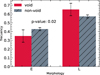 |
Fig. 4. Fraction of ETGs and LTGs in the void (red) and non-void (dashed gray) galaxy samples. Error bars indicate the 95% confidence intervals for each proportion. The figure also shows the p-value from a hypothesis test evaluating whether the proportions of early- and late-type galaxies differ significantly between void and non-void environments. |
To determine if these differences are significant, we tested whether the observed fraction of early-type (or late-type) galaxies in void environments could be due to random variation when compared to non-void environments. The test yields a p-value of 0.02, supporting the conclusion that both proportions differ significantly.
After separating the galaxies by morphology in both void and non-void samples, we studied their light-weighted stellar metallicity and age at the effective radius. In Fig. 5, we present violin plots for metallicity (top panel) and age (bottom panel). The distributions show that ETGs are typically more metal-rich and host older stellar populations compared to LTGs (Kauffmann et al. 2003; Gallazzi et al. 2005).
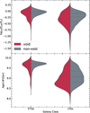 |
Fig. 5. Distribution of stellar properties for void and non-void galaxies, separated by ETGs and LTGs. Top panel: Stellar metallicity. Bottom panel: Galaxy age. In each panel, the left distribution shows ETGs and the right distribution shows LTGs. In each violin plot, the left (red) side represents the void galaxy sample, while the right (gray) side represents the non-void sample. Solid lines within the violin plots indicate the median values and the 25th–75th percentiles. |
For ETGs, although the void and non-void distributions show the same median values for age and metallicity, we observe a tail in the void sample distributions extending toward lower values for both properties. In the case of LTGs, the distributions appear significantly different. The metallicity distributions suggest a bimodality for the void sample, with a more pronounced low-metallicity peak. Regarding the age distribution, the void sample is skewed towards younger ages in comparison with the non-void sample. The medians in both panels indicate that the void sample has lower metallicities and younger ages for LTGs than the non-void galaxy sample.
We note that aside from morphology, we also investigated whether the gas content of galaxies varies with environment for both morphological types. Our analysis did not reveal any significant differences in gas content between void and non-void galaxies, leading us to focus our discussion and figures on the stellar properties instead.
3.3. Age and metallicity distributions
In the previous subsection, we demonstrated that the distribution of ETGs and LTGs differs according to both morphological type and environment. However, it is important to emphasize that the r-band absolute magnitude distributions of the void and non-void samples differ. As shown in Fig. 1, the void sample distribution is skewed toward fainter magnitudes compared to the non-void sample. Typically, the brighter a galaxy is, the richer its stellar population is in metals. Therefore, the observed differences in metallicity and age in Fig. 5 could be more closely related to differences in galaxy magnitude rather than their environmental location. To avoid this bias, we generated a new non-void galaxy sample that matches the r-band absolute magnitude distribution of the void sample. Since the non-void sample contains many more galaxies, we can replicate the magnitude distribution with ten times more galaxies, which helps to reduce statistical errors.
In Fig. 6, we present the metallicity distribution (left panel) and age distribution (right panel) for void galaxies (red histograms) and the new non-void sample (gray histograms) that mimics the r-band magnitude void distribution. Both distributions indicate that void galaxies are less metal-rich and younger than non-void galaxies. This is reflected in the median values shown in the plots and the p-values resulting from a Kolmogorov-Smirnov (KS) test, which indicate that, in both cases, the distributions for void and non-void galaxies are statistically different.
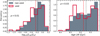 |
Fig. 6. Left panel: Distribution of stellar metallicity for a sample of non-void galaxies that mimics the r-band absolute magnitude distribution of void galaxies. Right panel: The galaxy age distribution for the same samples. The filled gray histogram represents the distribution for non-void galaxies, while the red histogram represents the distribution for void galaxies. A vertical dotted black line indicates the median for the non-void sample, and a dashed red line indicates the median for the void sample in each panel. Each panel also includes the p-value from the KS statistical test. |
3.4. Galaxy gradients
Following the methodology outlined in the previous section, we analyze the metallicity and age profiles of ETGs and LTGs, ensuring that the absolute magnitude distribution of void galaxies matches that of non-void galaxies. The profiles were constructed using the data presented in Riffel et al. (2023) (MEGACUBES) and explained in Section 2.2, where stellar metallicities and ages for each galaxy were calculated in concentric bins centered on the galaxy, extending out to 2 Re or 1.5 Re, depending on whether the galaxy belongs to the PS or SS (Yan et al. 2016; Wake et al. 2017).
We mimic the r-band magnitude distribution of void galaxies using non-void galaxies and stack all galaxies in both samples. The profiles are computed in units of the effective radius, which allows us to normalize galaxy sizes. From these stacked galaxies, we calculate the mean value in each bin to construct the mean profiles. Specifically, the mean value and associated error are calculated at radii of 0.5, 1.0, 1.5, and 2.0 Re. Since some galaxies have their properties measured only up to 1.5 Re (mainly those from the PS), the outermost bin is derived from a reduced subset of galaxies.
The results of these galaxy profiles are presented in Fig. 7. The left panels show the results for ETGs, while the right panels correspond to LTGs. For ETGs, in the top panel, void galaxies systematically exhibit lower metallicity values compared to non-void galaxies. The same trend is observed for stellar age. On average, for both metallicity and age, the results suggest a difference between void and non-void galaxies with a significance of approximately ∼1σ. For LTGs, the top right panel shows that void galaxies exhibit a slight negative metallicity gradient, while the non-void sample shows a more pronounced negative gradient in the profile, with more metal-rich bulges. However, the differences in the mean profiles lie within the error bars of the void sample. The bottom panel shows the stellar ages, where we observe a negative gradient for both void and non-void galaxies. The figure shows that void galaxies consistently exhibit lower stellar ages, particularly in the outer regions of the disk, where the differences exceed the associated error. We observe that, regardless of the environment, both early- and late-type galaxies exhibit negative age and metallicitygradients, consistent with the inside-out scenario (Pérez et al. 2013; González Delgado et al. 2014; García-Benito et al. 2017).
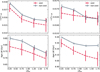 |
Fig. 7. Profiles of the mean stellar metallicity (top panels) and stellar age (bottom panels). The left-hand panels correspond to ETGs, and the right-hand panels to LTGs. Void galaxies are shown with dashed red lines, while non-void galaxies are shown with solid gray line. Error bars indicate the uncertainty in the mean, calculated as |

For comparison with other studies, we computed the metallicity gradients ∇[Z/H] and age gradients for our samples using the 0.25−1.25 Re interval. In the case of metallicity, the gradients were calculated on a logarithmic scale, adopting a solar metallicity of Z⊙ = 0.017. For LTGs, the metallicity gradients are ∇[Z/H] = 0.006 ± 0.014 (void sample) and ∇[Z/H] = −0.016 ± 0.005 (non-void sample). For ETGs, the metallicity gradients are ∇[Z/H] = −0.053 ± 0.021 (void sample) and ∇[Z/H] = −0.053 ± 0.006 (non-void sample). All metallicity gradients are expressed in units of [dex/Re]. For the age gradients, we obtain the following values for LTGs: ∇Age = −0.217 ± 0.005 (void sample) and ∇Age = −0.142 ± 0.001 (non-void sample). For ETGs, the gradients are ∇Age = −0.056 ± 0.003 (void sample) and ∇Age = −0.063 ± 0.001 (non-void sample). In this case, the units of these gradients are [log10(Gyr)/Re].
For each MaNGA megacube, Riffel et al. (2023) calculated the binned population vectors, which represent the fractional contribution of stellar populations in different age ranges. These are defined as follows:
-
xyy light: t ≤ 10 Myr
-
xyo light: 14 Myr < t ≤ 56 Myr
-
xiy light: 100 Myr < t ≤ 500 Myr
-
xii light: 630 Myr < t ≤ 800 Myr
-
xio light: 890 Myr < t ≤ 2.0 Gyr
-
xo light: 5.0 Gyr < t ≤ 13 Gyr.
The letters denote groups: y (young), i (intermediate), and o (old). To simplify our results, we group the vectors into three categories– young, intermediate, and old–defined as follows:
-
young: t ≤ 56 Myr
-
intermediate: 100 Myr < t ≤ 2 Gyr
-
old: 5 Gyr < t ≤ 13 Gyr.
In Fig. 8, we show the population profiles for these three categories, separated by morphological type (ETGs in the left panels, LTGs in the right). The top panels show the young population. For ETGs, the figure shows a younger population in all bins for void galaxies. The intermediate-age population is also higher in the void sample compared to the non-void sample. Conversely, the old stellar population shows higher fractions in the non-void sample. The trends are consistently observed, indicating younger stellar populations in void galaxies across all radial bins.
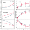 |
Fig. 8. Profiles of the mean fraction of stars in different age bins for early-type (left column) and late-type galaxies (right column). The top panels shows the young population (t < 56 Myr), the central panels show the intermediate population (100 Myr < t < 2 Gyr), and the bottom panels show the old population (2 Gyr < t < 5 Gyr). Void galaxies are shown with dashed red lines, and non-void galaxies with solid gray lines. Error bars indicate the uncertainty in the mean, calculated as |

For LTGs, the profile for void galaxies exhibits a higher fraction of young populations compared to the non-void sample. For the intermediate-age population (central panel), we find no significant differences between the void and non-void samples. In the old populations (bottom panel), the non-void sample displays higher fractions of these populations than the void sample.
4. Discussions
Our results with MaNGA data are consistent with previous studies analyzing the characteristics of galaxies in cosmic voids from various surveys. However, our findings provide a new perspective by utilizing IFS data from the MaNGA survey, which allows for more detailed modeling of stellar populations compared to traditional fiber spectroscopy or photometrical methods. In our analysis, we observed that void galaxies have lower absolute magnitudes and are bluer than galaxies in denser environments. We also identified a trend indicating that void galaxies exhibit higher SFRs. All of these results are in agreement with the general consensus on void galaxy properties (Rojas et al. 2004; Patiri et al. 2006; Tavasoli et al. 2015; Rodríguez-Medrano et al. 2023).
Our findings also show that, as a function of r-band absolute magnitude, void galaxies tend to have lower stellar metallicities than non-void galaxies. For the brighter galaxies, the difference is not statistically significant, indicating that the metallicities are similar in both environments. In Rodríguez-Medrano et al. (2024), we analyze the void galaxy population in the IllustrisTNG simulation and found a similar result: void galaxies exhibit lower stellar metallicities, with the signal decreasing as the stellar mass increases. The same trend was found in the SDSS-DR7 data in Domínguez-Gómez et al. (2023b). Given that stellar mass correlates with absolute magnitude, our results in this paper are consistent with those in previous works.
We also explored whether void galaxies have a higher gas content compared to galaxies in denser environments, as suggested in Rodríguez-Medrano et al. (2024). However, we did not find a dependence of the gas content on the environment. Across the entire range of absolute magnitudes analyzed, galaxies displayed the same mean gas masses. One of the main results from the work of Florez et al. (2021) is that void galaxies are richer in gas, even when controlling for the morphology and mass of the galaxies. In their study, the gas mass is derived either directly from the HI data for some galaxies or indirectly through a relation between the galaxy color and the gas mass fraction. Beyond the differences in the determination of the gas mass between both studies, the definition of voids also differs. In their work, galaxies are classified as void and non-void based on their distance to the nearest neighboring galaxies, making this classification dependent on the local environment, in contrast to our classification, which is based on the integrated large-scale density field. Another study investigating the gas content in void galaxies is Domínguez-Gómez et al. (2022), where no significant differences in gas mass are found between a sample of void galaxies and a control sample of galaxies in denser environments. In this study, the void galaxy sample is selected based on the large-scale density field, making their void galaxy definition more comparable to that of our samples. Despite differences among the various studies in the literature, it would be valuable to include a sample of fainter galaxies in future analyses, as the differences in gas content predicted in our numerical work Rodríguez-Medrano et al. (2024) are expected to be more significant in low-mass galaxies, consistent with our previous finding. On the other hand, we emphasize that the gas mass estimates used in this work depend on properties such as galaxy inclination and SFR (Barrera-Ballesteros et al. 2021). A detailed analysis of the gas content in galaxies should not only control for global magnitudes, as we have done here, but also ensure that the samples are unbiased with respect to inclination and SFR. Considering these factors, and the fact that we restricted our analysis to the SS to ensure consistent spatial coverage across galaxies, the results related to gas mass should be interpreted with appropriate caution.
As noted in the introduction, a high proportion of LTGs is expected in cosmic voids (Hoyle et al. 2005; Ricciardelli et al. 2017). In our data, we find that the fraction of LTGs is slightly higher in void environments (65%) compared to non-void environments (57%). We obtain a p-value of p = 0.02, supporting the hypothesis that voids host a higher fraction of LTGs in voids compared to denser environments.
When analyzing the distribution of metallicity by morphological type (Fig. 5), we find that ETGs in both void and non-void environments generally exhibit higher light-weightedstellar metallicities than LTGs. However, the metallicity distribution for void environments shows a bimodal behavior, with a smaller population of galaxies at lower metallicities. For LTGs, void galaxies tend to have lower stellar metallicities and also exhibit a bimodal distribution. For the light-weighted age (LW-age) distributions, ETGs display similar patterns in both environments. In contrast, LTGs show differing distributions, with void galaxies skewed toward younger ages, suggesting a younger population of galaxies. These differences in age and metallicity in late-type galaxies persist even in samples with the same magnitude distribution, confirming an environmental effect and not simply a bias due to the magnitude of galaxies.
The galaxy metallicity profiles presented in Fig. 7 exhibit negative gradients for LTGs in both void and non-void samples, with the gradient being more pronounced in non-void galaxies. However, these two behaviors are not statistically distinguishable when considering the errors in the calculated gradients. For ETGs, we found a trend suggesting a less metal-rich stellar population across the entire range of distances for the void galaxy population.
The age profiles for LTGs and ETGs consistently indicate younger populations in void galaxies. For ETGs, the profiles are similar but display an offset to lower values in the void environment. For LTGs, the gradients appear to differ in the outer regions (disks), indicating similar bulges in both void and non-void environments, but suggesting that the disks of void galaxies host a younger population.
A recent study on the relationship between age gradients and the environment of voids is presented by Conrado et al. (2024). In that work, the authors use a sample of void galaxies and a control sample, classifying them morphologically as E, S0, Sa, Sb, Sc, and Sd. When comparing both samples, they find that, for all morphological types, the age profiles indicate that void galaxies have younger stellar populations. In our case, due to the limited number of galaxies, we classified them into only two morphological types: ETGs and LTGs. Nevertheless, our results qualitatively agree with those reported by Conrado et al. (2024).
Overall, our results indicate that void galaxies are younger and possess lower stellar metallicities. The age findings are consistent with those obtained from simulations (Tonnesen & Cen 2015; Alfaro et al. 2020; Rodríguez Medrano et al. 2022; Rodríguez-Medrano et al. 2024) and observational studies (Domínguez-Gómez et al. 2023a; Torres-Ríos et al. 2024), which employed spectral distribution models on spectroscopic data. The observed difference in galaxy ages suggests that the lower metallicities in void galaxies may be attributed to their younger stellar populations.
Finally, we acknowledge several limitations of our study. The MaNGA galaxy sample, although the most extensive IFS survey conducted to date, is limited by its bias toward brighter galaxies, which may affect our results related to gas content and the properties of lower-mass galaxies. Furthermore, although the morphological separation into early and late types provides clarity, morphology can be classified in greater detail based on the Hubble sequence or different T-types. Nonetheless, we emphasize that our decision to focus solely on two morphological types was motivated by the need to achieve a statistically significant number of galaxies within each type, thereby enhancing the robustness of our results.
5. Conclusions
In this paper, we analyzed IFS data from the MaNGA survey, separating galaxies into those located within cosmic voids and those outside. The main findings of this work can be summarized as follows:
-
At a given absolute magnitude, void galaxies are younger and exhibit lower metallicities compared to galaxies in non-void environments.
-
The gas content of galaxies in voids and non-void environments is similar.
-
When matching the absolute magnitude distribution of void galaxies with that of non-void galaxies, we find statistically significant evidence that the stellar metallicity and age distributions are different between the two samples. The comparison shows that void galaxies are younger and less metal-rich.
-
These differences in evolutionary signals are evident for both early- and late-type galaxies.
The results related to the metallicity and age of galaxies confirm some of the key findings obtained through numerical simulations in Rodríguez-Medrano et al. (2024). However, we did not find differences in the gas content of void galaxies, which was one of the objectives of this study. This may be due to the requirement for a sample with lower-mass galaxies than those used here.
In conclusion, we have shown how the void environment affects galaxy evolution, influencing star formation activity. Our results suggest a delayed evolutionary path for galaxies in large-scale underdense environments, which is reflected in a younger stellar population and lower metallicities.
Acknowledgments
The authors thank the referee for reviewing the manuscript and for their helpful comments and suggestions. ARM thanks Ornela Marioni for the valuable discussions held during the preparation of this work. This work was partially supported by grants PICT 2021-00442 awarded by Fondo para la Investigación Científica y Tecnológica (FONCYT), grant PIP 2022-11220210100520 by the Consejo de Investigaciones Científicas y Técnicas de la República Argentina (CONICET), and the Secretaría de Ciencia y Técnica de la Universidad Nacional de Córdoba (SeCyT). ARM is doctoral fellow of CONICET. DJP, DM, ANR, and FAS are members of the Carrera del Investigador Científico (CONICET). This project makes use of the MaNGA-Pipe3D dataproducts. We thank the IA-UNAM MaNGA team for creating this catalog, and the Conacyt Project CB-285080 for supporting them. Funding for the Sloan Digital Sky Survey IV has been provided by the Alfred P. Sloan Foundation, the U.S. Department of Energy Office of Science, and the Participating Institutions. SDSS-IV acknowledges support and resources from the Center for High Performance Computing at the University of Utah. The SDSS website is www.sdss4.org. SDSS-IV is managed by the Astrophysical Research Consortium for the Participating Institutions of the SDSS Collaboration including the Brazilian Participation Group, the Carnegie Institution for Science, Carnegie Mellon University, Center for Astrophysics | Harvard & Smithsonian, the Chilean Participation Group, the French Participation Group, Instituto de Astrofísica de Canarias, The Johns Hopkins University, Kavli Institute for the Physics and Mathematics of the Universe (IPMU)/University of Tokyo, the Korean Participation Group, Lawrence Berkeley National Laboratory, Leibniz Institut für Astrophysik Potsdam (AIP), Max-Planck-Institut für Astronomie (MPIA Heidelberg), Max-Planck-Institut für Astrophysik (MPA Garching), Max-Planck-Institut für Extraterrestrische Physik (MPE), National Astronomical Observatories of China, New Mexico State University, New York University, University of Notre Dame, Observatário Nacional/MCTI, The Ohio State University, Pennsylvania State University, Shanghai Astronomical Observatory, United Kingdom Participation Group, Universidad Nacional Autónoma de México, University of Arizona, University of Colorado Boulder, University of Oxford, University of Portsmouth, University of Utah, University of Virginia, University of Washington, University of Wisconsin, Vanderbilt University, and Yale University.
References
- Abazajian, K. N., Adelman-McCarthy, J. K., Agüeros, M. A., et al. 2009, ApJS, 182, 543 [Google Scholar]
- Alam, S., Albareti, F. D., Allende Prieto, C., et al. 2015, ApJS, 219, 12 [Google Scholar]
- Alfaro, I. G., Rodriguez, F., Ruiz, A. N., & Lambas, D. G. 2020, A&A, 638, A60 [NASA ADS] [CrossRef] [EDP Sciences] [Google Scholar]
- Argudo-Fernández, M., Gómez Hernández, C., Verley, S., et al. 2024, A&A, 692, A258 [NASA ADS] [CrossRef] [EDP Sciences] [Google Scholar]
- Bacon, R., Copin, Y., Monnet, G., et al. 2001, MNRAS, 326, 23 [Google Scholar]
- Barrera-Ballesteros, J. K., Heckman, T., Sánchez, S. F., et al. 2021, ApJ, 909, 131 [NASA ADS] [CrossRef] [Google Scholar]
- Brinchmann, J., Charlot, S., White, S. D. M., et al. 2004, MNRAS, 351, 1151 [Google Scholar]
- Bundy, K., Bershady, M. A., Law, D. R., et al. 2015, ApJ, 798, 7 [Google Scholar]
- Ceccarelli, L., Padilla, N., & Lambas, D. G. 2008, MNRAS, 390, L9 [NASA ADS] [Google Scholar]
- Cid Fernandes, R. 2018, MNRAS, 480, 4480 [NASA ADS] [CrossRef] [Google Scholar]
- Cid Fernandes, R., Mateus, A., Sodré, L., Stasińska, G., & Gomes, J. M. 2005, MNRAS, 358, 363 [Google Scholar]
- Conrado, A. M., González Delgado, R. M., García-Benito, R., et al. 2024, A&A, 687, A98 [NASA ADS] [CrossRef] [EDP Sciences] [Google Scholar]
- Croom, S. M., Lawrence, J. S., Bland-Hawthorn, J., et al. 2012, MNRAS, 421, 872 [NASA ADS] [Google Scholar]
- Curtis, O., McDonough, B., & Brainerd, T. G. 2024, ApJ, 962, 58 [NASA ADS] [CrossRef] [Google Scholar]
- Dey, A., Schlegel, D. J., Lang, D., et al. 2019, AJ, 157, 168 [Google Scholar]
- Domínguez-Gómez, J., Lisenfeld, U., Pérez, I., et al. 2022, A&A, 658, A124 [NASA ADS] [CrossRef] [EDP Sciences] [Google Scholar]
- Domínguez-Gómez, J., Pérez, I., Ruiz-Lara, T., et al. 2023a, A&A, 680, A111 [NASA ADS] [CrossRef] [EDP Sciences] [Google Scholar]
- Domínguez-Gómez, J., Pérez, I., Ruiz-Lara, T., et al. 2023b, Nature, 619, 269 [CrossRef] [Google Scholar]
- Douglass, K. A., Smith, J. A., & Demina, R. 2019, ApJ, 886, 153 [Google Scholar]
- Florez, J., Berlind, A. A., Kannappan, S. J., et al. 2021, ApJ, 906, 97 [NASA ADS] [CrossRef] [Google Scholar]
- Gallazzi, A., Charlot, S., Brinchmann, J., White, S. D. M., & Tremonti, C. A. 2005, MNRAS, 362, 41 [Google Scholar]
- García-Benito, R., González Delgado, R. M., Pérez, E., et al. 2017, A&A, 608, A27 [NASA ADS] [CrossRef] [EDP Sciences] [Google Scholar]
- González Delgado, R. M., Cerviño, M., Martins, L. P., Leitherer, C., & Hauschildt, P. H. 2005, MNRAS, 357, 945 [Google Scholar]
- González Delgado, R. M., Pérez, E., Cid Fernandes, R., et al. 2014, A&A, 562, A47 [CrossRef] [EDP Sciences] [Google Scholar]
- Habouzit, M., Pisani, A., Goulding, A., et al. 2020, MNRAS, 493, 899 [NASA ADS] [CrossRef] [Google Scholar]
- Hoyle, F., Rojas, R. R., Vogeley, M. S., & Brinkmann, J. 2005, ApJ, 620, 618 [NASA ADS] [CrossRef] [Google Scholar]
- Hoyle, F., Vogeley, M. S., & Pan, D. 2012, MNRAS, 426, 3041 [NASA ADS] [CrossRef] [Google Scholar]
- Ibarra-Medel, H. J., Sánchez, S. F., Avila-Reese, V., et al. 2016, MNRAS, 463, 2799 [NASA ADS] [CrossRef] [Google Scholar]
- Kauffmann, G., Heckman, T. M., White, S. D. M., et al. 2003, MNRAS, 341, 33 [Google Scholar]
- Kennicutt, R. C. 1998, ARA&A, 36, 189 [NASA ADS] [CrossRef] [Google Scholar]
- Kreckel, K., Platen, E., Aragón-Calvo, M. A., et al. 2011, AJ, 141, 4 [NASA ADS] [CrossRef] [Google Scholar]
- Lacerda, E. A. D., Sánchez, S. F., Mejía-Narváez, A., et al. 2022, New Astron., 97, 101895 [NASA ADS] [CrossRef] [Google Scholar]
- Martizzi, D., Vogelsberger, M., Torrey, P., et al. 2020, MNRAS, 491, 5747 [CrossRef] [Google Scholar]
- Moorman, C. M., Moreno, J., White, A., et al. 2016, ApJ, 831, 118 [NASA ADS] [CrossRef] [Google Scholar]
- Moustakas, J., Kennicutt, R. C., Tremonti, C. A., et al. 2010, ApJS, 190, 233 [NASA ADS] [CrossRef] [Google Scholar]
- Nelson, D., Springel, V., Pillepich, A., et al. 2019, Comput. Astrophys. Cosmol., 6, 2 [Google Scholar]
- Patiri, S. G., Prada, F., Holtzman, J., Klypin, A., & Betancort-Rijo, J. 2006, MNRAS, 372, 1710 [NASA ADS] [CrossRef] [Google Scholar]
- Pérez, E., Cid Fernandes, R., González Delgado, R. M., et al. 2013, ApJ, 764, L1 [Google Scholar]
- Pérez, I., Verley, S., Sánchez-Menguiano, L., et al. 2024, A&A, 689, A213 [NASA ADS] [CrossRef] [EDP Sciences] [Google Scholar]
- Pillepich, A., Nelson, D., Hernquist, L., et al. 2018, MNRAS, 475, 648 [Google Scholar]
- Porter, L. E., Holwerda, B. W., Kruk, S., et al. 2023, MNRAS, 524, 5768 [NASA ADS] [CrossRef] [Google Scholar]
- Ricciardelli, E., Cava, A., Varela, J., & Tamone, A. 2017, ApJ, 846, L4 [NASA ADS] [CrossRef] [Google Scholar]
- Riffel, R., Mallmann, N. D., Rembold, S. B., et al. 2023, MNRAS, 524, 5640 [NASA ADS] [CrossRef] [Google Scholar]
- Rodriguez, F., & Merchán, M. 2020, A&A, 636, A61 [NASA ADS] [CrossRef] [EDP Sciences] [Google Scholar]
- Rodríguez Medrano, A. M., Paz, D. J., Stasyszyn, F. A., & Ruiz, A. N. 2022, MNRAS, 511, 2688 [Google Scholar]
- Rodríguez-Medrano, A. M., Paz, D. J., Stasyszyn, F. A., et al. 2023, MNRAS, 521, 916 [CrossRef] [Google Scholar]
- Rodríguez-Medrano, A. M., Springel, V., Stasyszyn, F. A., & Paz, D. J. 2024, MNRAS, 528, 2822 [CrossRef] [Google Scholar]
- Rojas, R. R., Vogeley, M. S., Hoyle, F., & Brinkmann, J. 2004, ApJ, 617, 50 [NASA ADS] [CrossRef] [Google Scholar]
- Rojas, R. R., Vogeley, M. S., Hoyle, F., & Brinkmann, J. 2005, ApJ, 624, 571 [NASA ADS] [CrossRef] [Google Scholar]
- Rosas-Guevara, Y., Tissera, P., Lagos, C. D. P., Paillas, E., & Padilla, N. 2022, MNRAS, 517, 712 [NASA ADS] [CrossRef] [Google Scholar]
- Ruiz, A. N., Paz, D. J., Lares, M., et al. 2015, MNRAS, 448, 1471 [NASA ADS] [CrossRef] [Google Scholar]
- Ruiz, A. N., Alfaro, I. G., & Garcia Lambas, D. 2019, MNRAS, 483, 4070 [NASA ADS] [CrossRef] [Google Scholar]
- Ruschel-Dutra, D., & Dall’Agnol De Oliveira, B. 2020, https://doi.org/10.5281/zenodo.4065550 [Google Scholar]
- Ruschel-Dutra, D., Storchi-Bergmann, T., Schnorr-Müller, A., et al. 2021, MNRAS, 507, 74 [NASA ADS] [CrossRef] [Google Scholar]
- Sánchez, S. F., Kennicutt, R. C., Gil de Paz, A., et al. 2012, A&A, 538, A8 [Google Scholar]
- Sánchez, S. F., Pérez, E., Sánchez-Blázquez, P., et al. 2016a, Rev. Mex. Astron. Astrofis., 52, 171 [Google Scholar]
- Sánchez, S. F., Pérez, E., Sánchez-Blázquez, P., et al. 2016b, Rev. Mex. Astron. Astrofis., 52, 21 [NASA ADS] [Google Scholar]
- Sánchez, S. F., Barrera-Ballesteros, J. K., Lacerda, E., et al. 2022, ApJS, 262, 36 [CrossRef] [Google Scholar]
- Sánchez, S. F., García-Benito, R., González Delgado, R., et al. 2024, Rev. Mex. Astron. Astrofis., 60, 323 [Google Scholar]
- Scholz-Díaz, L., Martín-Navarro, I., & Falcón-Barroso, J. 2022, MNRAS, 511, 4900 [CrossRef] [Google Scholar]
- Scholz-Díaz, L., Martín-Navarro, I., & Falcón-Barroso, J. 2023, MNRAS, 518, 6325 [Google Scholar]
- Springel, V., Pakmor, R., Pillepich, A., et al. 2018, MNRAS, 475, 676 [Google Scholar]
- Tavasoli, S., Rahmani, H., Khosroshahi, H. G., Vasei, K., & Lehnert, M. D. 2015, ApJ, 803, L13 [Google Scholar]
- Tonnesen, S., & Cen, R. 2015, ApJ, 812, 104 [Google Scholar]
- Torres-Ríos, G., Pérez, I., Verley, S., et al. 2024, A&A, 691, A341 [NASA ADS] [CrossRef] [EDP Sciences] [Google Scholar]
- van de Weygaert, R., & Platen, E. 2011, Int. J. Mod. Phys. Conf. Ser., 1, 41 [NASA ADS] [CrossRef] [Google Scholar]
- Vazdekis, A., Sánchez-Blázquez, P., Falcón-Barroso, J., et al. 2010, MNRAS, 404, 1639 [NASA ADS] [Google Scholar]
- Vazdekis, A., Koleva, M., Ricciardelli, E., Röck, B., & Falcón-Barroso, J. 2016, MNRAS, 463, 3409 [Google Scholar]
- Vázquez-Mata, J. A., Hernández-Toledo, H. M., Avila-Reese, V., et al. 2022, MNRAS, 512, 2222 [CrossRef] [Google Scholar]
- von Benda-Beckmann, A. M., & Müller, V. 2008, MNRAS, 384, 1189 [CrossRef] [Google Scholar]
- Wake, D. A., Bundy, K., Diamond-Stanic, A. M., et al. 2017, AJ, 154, 86 [Google Scholar]
- Yan, R., Bundy, K., Law, D. R., et al. 2016, AJ, 152, 197 [Google Scholar]
- Yan, R., Chen, Y., Lazarz, D., et al. 2019, ApJ, 883, 175 [Google Scholar]
- York, D. G., Adelman, J., Anderson, J. E., et al. 2000, AJ, 120, 1579 [Google Scholar]
Appendix A: Samples characterization
In Fig. A.1, we present the distributions of redshift, effective radius, and inclination angle for our sample of galaxies (void and non-void). The figure shows similar distributions for the effective radius and inclination angle. The largest difference is observed in the redshift distribution. This difference arises from the variation in the magnitude of galaxies in both environments (see Fig. 1). In void environments, the galaxy distribution is biased towards faint galaxies, which cannot be observed at higher redshifts.
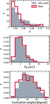 |
Fig. A.1. Properties of void and non-void sample of galaxies. Top panel: Redshift distribution, Central panel: Effective radius Re [arc], Bottom panel: Inclination angle. The gray distribution correspond to non-void galaxies and red to void galaxies. |
To ensure that the difference in the redshift distribution does not bias our results when comparing void and non-void galaxies, we show in Fig. A.2 the mean redshift as a function of r-band magnitude for both environments. This plot is analogous to those shown in Fig. 2 and Fig. 3. From this, we can see that the mean redshift in all magnitude bins is comparable, ensuring that no bias is introduced by differences in the redshift of galaxies.
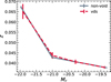 |
Fig. A.2. Mean redshift value as a function of r-band absolute magnitude. The dashed-red line indicate void galaxies and solid gray line correspond to the non-void sample. The error band indicate the error in the mean value. |
Figure A.3 shows the complete morphological type distribution of our samples. Irregular and Sm galaxies were excluded from the plot, as none belong to void environments. The figure illustrates that early-type galaxies (E and S0), as well as Sa, are more abundant in the non-void sample compared to void environments. In contrast, later-type galaxies (Sb, Sc, Sd) are more prevalent in the void sample.
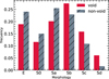 |
Fig. A.3. Distribution of morphological types (E, S0, Sa, Sb, Sc, Sd) for galaxies. With red bars we show the void galaxy sample and with dashed gray bars we show the non-void sample. |
All Figures
|
Fig. 1. Distribution of r-band absolute magnitudes for the galaxy samples. The filled gray histogram represents the non-void galaxy sample, while the red histogram shows the distribution for the void-galaxysample. |
| In the text | |
|
Fig. 2. Astrophysical properties of galaxies as a function of r-band absolute magnitude for void and non-void galaxies. Top panel: g − r color. Bottom panel: Star formation rate (SFR). Both panels show the relation for non-void galaxies (solid gray line) and void galaxies (dashed red line). Error bars indicate the uncertainty associated with the mean value. |
| In the text | |
|
Fig. 3. Astrophysical properties of galaxies as a function of r-band absolute magnitude. Top panel: Luminosity weighted stellar metallicity. Middle panel: Luminosity weighted galaxy age. Bottom panel: Gas mass for galaxies in the SS. The solid gray line represents the relation for the non-void galaxy sample, while the dashed red line represents the relation for the void galaxy sample. Error bars indicate the uncertainty associated with the mean value. |
| In the text | |
|
Fig. 4. Fraction of ETGs and LTGs in the void (red) and non-void (dashed gray) galaxy samples. Error bars indicate the 95% confidence intervals for each proportion. The figure also shows the p-value from a hypothesis test evaluating whether the proportions of early- and late-type galaxies differ significantly between void and non-void environments. |
| In the text | |
|
Fig. 5. Distribution of stellar properties for void and non-void galaxies, separated by ETGs and LTGs. Top panel: Stellar metallicity. Bottom panel: Galaxy age. In each panel, the left distribution shows ETGs and the right distribution shows LTGs. In each violin plot, the left (red) side represents the void galaxy sample, while the right (gray) side represents the non-void sample. Solid lines within the violin plots indicate the median values and the 25th–75th percentiles. |
| In the text | |
|
Fig. 6. Left panel: Distribution of stellar metallicity for a sample of non-void galaxies that mimics the r-band absolute magnitude distribution of void galaxies. Right panel: The galaxy age distribution for the same samples. The filled gray histogram represents the distribution for non-void galaxies, while the red histogram represents the distribution for void galaxies. A vertical dotted black line indicates the median for the non-void sample, and a dashed red line indicates the median for the void sample in each panel. Each panel also includes the p-value from the KS statistical test. |
| In the text | |
|
Fig. 7. Profiles of the mean stellar metallicity (top panels) and stellar age (bottom panels). The left-hand panels correspond to ETGs, and the right-hand panels to LTGs. Void galaxies are shown with dashed red lines, while non-void galaxies are shown with solid gray line. Error bars indicate the uncertainty in the mean, calculated as |
| In the text | |
|
Fig. 8. Profiles of the mean fraction of stars in different age bins for early-type (left column) and late-type galaxies (right column). The top panels shows the young population (t < 56 Myr), the central panels show the intermediate population (100 Myr < t < 2 Gyr), and the bottom panels show the old population (2 Gyr < t < 5 Gyr). Void galaxies are shown with dashed red lines, and non-void galaxies with solid gray lines. Error bars indicate the uncertainty in the mean, calculated as |
| In the text | |
|
Fig. A.1. Properties of void and non-void sample of galaxies. Top panel: Redshift distribution, Central panel: Effective radius Re [arc], Bottom panel: Inclination angle. The gray distribution correspond to non-void galaxies and red to void galaxies. |
| In the text | |
|
Fig. A.2. Mean redshift value as a function of r-band absolute magnitude. The dashed-red line indicate void galaxies and solid gray line correspond to the non-void sample. The error band indicate the error in the mean value. |
| In the text | |
|
Fig. A.3. Distribution of morphological types (E, S0, Sa, Sb, Sc, Sd) for galaxies. With red bars we show the void galaxy sample and with dashed gray bars we show the non-void sample. |
| In the text | |
Current usage metrics show cumulative count of Article Views (full-text article views including HTML views, PDF and ePub downloads, according to the available data) and Abstracts Views on Vision4Press platform.
Data correspond to usage on the plateform after 2015. The current usage metrics is available 48-96 hours after online publication and is updated daily on week days.
Initial download of the metrics may take a while.