| Issue |
A&A
Volume 700, August 2025
|
|
|---|---|---|
| Article Number | A216 | |
| Number of page(s) | 16 | |
| Section | Planets, planetary systems, and small bodies | |
| DOI | https://doi.org/10.1051/0004-6361/202553719 | |
| Published online | 20 August 2025 | |
Discovery of a transiting hot water-world candidate orbiting Ross 176 with TESS and CARMENES
1
Instituto de Astrofísica de Canarias (IAC),
38205
La Laguna,
Tenerife,
Spain
2
Departamento de Astrofísica, Universidad de La Laguna (ULL),
38206
La Laguna,
Tenerife,
Spain
3
Department of Astronomy, University of Texas at Austin,
2515 Speedway,
Austin,
TX
78712,
USA
4
Centro de Astrobiología (CSIC-INTA),
Camino Bajo del Castillo s/n, Campus ESAC,
28692
Villanueva de la Cañada,
Madrid,
Spain
5
Departamento de Física de la Tierra y Astrofísica & IPARCOS-UCM (Instituto de Física de Partículas y del Cosmos de la UCM), Facultad de Ciencias Físicas, Universidad Complutense de Madrid,
28040
Madrid,
Spain
6
Instituto de Astrofísica de Andalucía (IAA-CSIC),
Glorieta de la Astronomía s/n,
18008
Granada,
Spain
7
Institut für Astrophysik und Geophysik, Georg-August-Universität,
Friedrich-Hund-Platz 1,
37077
Göttingen,
Germany
8
Hamburger Sternwarte,
Gojenbergsweg 112,
21029
Hamburg,
Germany
9
Komaba Institute for Science, The University of Tokyo,
3-8-1 Komaba,
Meguro,
Tokyo
153-8902,
Japan
10
Department of Multi-Disciplinary Sciences, Graduate School of Arts and Sciences, The University of Tokyo,
3-8-1 Komaba,
Meguro,
Tokyo,
Japan
11
Department of Astronomy & Astrophysics, University of Chicago,
Chicago,
IL
60637,
USA
12
Astrobiology Center,
2-21-1 Osawa,
Mitaka,
Tokyo
181-8588,
Japan
13
National Astronomical Observatory of Japan,
2-21-1 Osawa,
Mitaka,
Tokyo
181-8588,
Japan
14
Aristotle University of Thessaloniki,
University Campus,
54124,
Thessaloniki,
Greece
15
Institut de Ciències de l’Espai (ICE, CSIC),
Campus UAB, c/de Can Magrans s/n,
08193
Bellaterra,
Barcelona,
Spain
16
Institut d’Estudis Espacials de Catalunya (IEEC),
08860
Castellde-fels (Barcelona),
Spain
17
Steward Observatory and Department of Astronomy, The University of Arizona,
Tucson,
AZ
85721,
USA
18
Department of Physics and Kavli Institute for Astrophysics and Space Research, Massachusetts Institute of Technology,
Cambridge,
MA
02139,
USA
19
Department of Earth, Atmospheric and Planetary Sciences, Massachusetts Institute of Technology,
Cambridge,
MA
02139,
USA
20
Department of Aeronautics and Astronautics, MIT,
77 Massachusetts Avenue,
Cambridge,
MA
02139,
USA
21
Department of Physics and Astronomy, Vanderbilt University,
Nashville,
TN
37235,
USA
22
Landessternwarte, Zentrum für Astronomie der Universtät Heidelberg,
Königstuhl 12,
69117
Heidelberg,
Germany
23
Department of Astronomy, Faculty of Physics, Sofia University “St. Kliment Ohridski”,
5 James Bourchier Blvd.,
BG-1164
Sofia,
Bulgaria
24
Vereniging Voor Sterrenkunde,
Oude Bleken 12,
2400
Mol,
Belgium
25
AstroLAB IRIS, Provinciaal Domein “De Palingbeek”,
Verbrande-molenstraat 5,
8902
Zillebeke,
Ieper,
Belgium
26
Centre for Mathematical Plasma-Astrophysics, Department of Mathematics, KU Leuven,
Celestijnenlaan 200B,
3001
Heverlee,
Belgium
27
Department of Astrophysical Sciences, Princeton University,
Princeton,
NJ
08544,
USA
★ Corresponding author: This email address is being protected from spambots. You need JavaScript enabled to view it.
Received:
10
January
2025
Accepted:
25
June
2025
Abstract
The Transiting Exoplanet Survey Satellite (TESS) discovered several new planet candidates that need to be confirmed and characterized with ground-based observations. This is the case of Ross 176, a late K-type star that hosts a promising water-world candidate planet. The star has a radius of R⋆ = 0.569 ± 0.020 R⊙ and a mass of M⋆ = 0.577 ± 0.024 M⊙. We constrained the planetary mass using spectroscopic data from CARMENES, an instrument that has already played a major role in confirming the planetary nature of the transit signal detected by TESS. We used Gaussian Processes (GP) to improve the analysis because the host star has a relatively strong activity that affects the radial velocity dataset. In addition, we applied a GP to the TESS light curves to reduce the correlated noise in the detrended dataset. The stellar activity indicators show a strong signal that is related to the stellar rotation period of ∼32 days. This stellar activity signal was also confirmed on the TESS light curves. Ross 176 b is an inner hot transiting planet with a low-eccentricity orbit of e = 0.25 ± 0.04, an orbital period of P ~ 5 days, and an equilibrium temperature of Teq ~ 682 K. With a radius of Rp = 1.84 ± 0.08 R⊕ (4% precision), a mass of Mp = 4.57−0.93+0.89M⊕ (20% precision), and a mean density of ρp = 4.03−0.81+0.49g cm−3, the composition of Ross 176 b might be consistent with a water-world scenario. Moreover, Ross 176 b is a promising target for atmospheric characterization, which might lead to more information on the existence, formation and composition of water worlds. This detection increases the sample of planets orbiting K-type stars. This sample is valuable for investigating the valley of planets with small radii around this type of star. This study also shows that the dual detection of space- and ground-based telescopes is efficient for confirm new planets.
Key words: planets and satellites: composition / planets and satellites: detection / planets and satellites: individual: Ross 176
NHFP Sagan Fellow.
© The Authors 2025
 Open Access article, published by EDP Sciences, under the terms of the Creative Commons Attribution License (https://creativecommons.org/licenses/by/4.0), which permits unrestricted use, distribution, and reproduction in any medium, provided the original work is properly cited.
This article is published in open access under the Subscribe to Open model. This email address is being protected from spambots. You need JavaScript enabled to view it. to support open access publication.
1 Introduction
The Transiting Exoplanet Survey Satellite (TESS; Ricker et al. 2015) was launched by NASA in April 2018. Currently, TESS is in its second extension until September 2025. The main goal of the mission is the exploration of exoplanets, and it is especially helpful in the search for planets smaller than 4 R⊕ (e.g., Lacedelli et al. 2024; Goffo et al. 2024; Murgas et al. 2024, among many other recent and previous discoveries).
Recent studies indicated that the small exoplanet population can be distinguished into two classifications: rocky super-Earths, and gas-dominated sub-Neptunes. The two populations seem to be divided by a radius valley (Fulton & Petigura 2018). This valley of planets with small radius is a notable paucity of planets whose radii are between 1.5 R⊕ and 2R⊕. Alternatively, Luque & Pallé (2022) proposed dividing the small exoplanets according to their relative density: rocky planets with an Earth-like composition, and water-rich planets (or water worlds). This proposed classification applied only to planets orbiting M-type stars. Its applicability to FGK stars remains uncertain, however, because only a few small planets (R < 4 R⊕) have precise mass measurements, particularly, small planets around K-type hosts (Lillo-Box et al. 2022). A larger number of planets with well-determined masses and radii is needed to understand the small-planet population across spectral types.
Moreover, Lingam & Loeb (2017) proposed to focus the exoplanet hunt on K- and G-type stars, in particular, on dwarfs one. The auhtors concluded that the best host stars of potential Earth analogs with complex biospheres similar to that of the Earth have stellar masses in the range 0.38 M⊙ < M⋆ < 1 M⊙, showing a peak at 0.55 M⊙. In particular, late K-type stars emit significantly weaker ultraviolet (UV) radiation than G-type stars, which reduces the risk of atmospheric erosion and enhances the stability of planetary atmospheres over time (Segura et al. 2005). This moderate UV environment is particularly advantageous for planets with substantial water content, such as water-world planets, because it minimizes the risk of photodissociation of water molecules, which might preserve the surface or subsurface oceans (Lingam & Loeb 2019).
The UV radiation from late K-type host stars can also affect the planets in the habitability zone, however, Richey-Yowell et al. (2022) analyzed the evolutionary trends of K stars by studying their strong spectral lines in the UV wavelengths. They concluded that this radiation decreases with age earlier than in M stars (≲650 Myr). Therefore, late K-type stars are more suitable hosts for planets that can sustain life than M-type stars (Rimmer et al. 2018). These lower UV levels make late K-type stars ideal for hosting planets with stable, long-term water reservoirs, and they might allow for the evolution of complex biospheres in a range of planetary compositions.
Some examples of super-Earth planets orbiting K-type stars are HD 40307 b (Tuomi et al. 2013), Kepler-62 b, c, d, e, and f (Borucki et al. 2013), and Wolf 503b (Polanski et al. 2021). Evolutionary models of the habitability of water worlds such as HD 40307 b indicate that the climates of these worlds are stable when the temperature changes due to different mechanisms (Kite & Ford 2018). The habitable water surface can last for several gigayears, and approximately 25% of the water worlds might contain a habitable water surface for more than 1 Gyr.
This study focuses on the characterization of Ross 176 b, a transiting water-world candidate exoplanet orbiting a late-type star in the K–M boundary. The paper is organized as follows: In Sects. 2 and 3 we describe the observations we used in this work. The stellar properties of Ross 176 are reported in Sect. 4. In Sect. 5 we explain the methods we used in the data analysis and the results we obtained. The discussion and conclusions are presented in Sects. 6 and 7, respectively.
2 TESS photometry
Ross 176 was listed in the TESS Input Catalogue (TIC; Stassun et al. 2018) as TIC 193336820. When a transit-like event was detected, however, it was alerted as a TESS object of interest TOI-4491. The star was observed in sectors 14, 15, 41, 55, and 56 with a cadence integration of 2 min. Sectors 14 and 15 were observed in August 2019, Sector 41 in August 2021, Sector 55 in August 2022, and Sector 56 in September 2022.
TESS raw data were processed by the TESS Science Processing Operation Center (SPOC; Jenkins et al. 2016), which provided two photometric reductions, simple aperture photometry (SAP; Morris et al. 2020), and pre-search data conditioning SAP (PDC-SAP; Smith et al. 2012; Stumpe et al. 2012, 2014), which are publicly available at the Mikulski Archive for Space Telescopes (MAST1). We analyzed the PDC-SAP flux for the transit analysis and the SAP flux data for the stellar activity analysis. A potential exoplanet candidate signal with a period of 5 days and a transit depth (∆F) of 1150 ppm, corresponding to a planet radius of ∼2.1 R⊕, was detected using the quick-look pipeline (QLP; Huang et al. 2020a,b). TESS light curves (LCs) show an average of five transits per sector.
Additionally, we checked all target pixel files (TPF) of TESS data for each sector (see Fig. A.1; Aller et al. 2020). Because no comparably bright stars lie inside the TESS apertures with a magnitude difference of five magnitudes and because the PDC-SAP flux is also corrected for dilution, we fixed the dilution factor to unity.
3 Ground-based follow-up observations
3.1 Ground-based photometry
Ross 176 was followed-up with the Multi-color Simultaneous Camera for studying Atmospheres of Transiting planets (MuS-CAT2; Narita et al. 2019), which is located at the Telescopio Carlos Sánchez (TCS) at the Observatorio del Teide on the island of Tenerife, Spain. MuSCAT2 has four cameras that work simultaneously in the g′, r′, i′, and zs′ band, and it obtains four LCs in one single observation. The raw images from each CCD (i.e., filter) were reduced following the standard procedure via the MuSCAT2 pipeline as described by Parviainen et al. (2020) and Parviainen (2022).
Although three transit opportunities of Ross 176 b were observed, one transit was excluded due to bad weather conditions. The MuSCAT2 photometric data provide evidence for a transit with a significance of 2.69σ, 2.37σ, 3.37σ, and 3.53σ ppt for the g′, r′, i′, and zs′ band, respectively (see Fig. A.2). The two MuSCAT2 transits are included in our analysis in Sect. 5.
The multicolor LCs were analyzed through a global optimization that accounted for the transit and baseline variations simultaneously using a linear combination of covariates (Parviainen et al. 2019; Parviainen et al. 2020). As a results of differences in the quality and scattering between space- and ground-based measurements, we analyzed the MuS-CAT2 datasets individually with an independent quadratic limbdarkening parameterization, relative flux offset, and additional jitter terms.
3.2 Spectroscopy with CARMENES
Spectroscopic observations were obtained with the Calar Alto high-Resolution search for M dwarfs with Exoearths with Near-infrared and optical Échelle Spectrographs (CARMENES; Quirrenbach et al. 2014), which is located at the Observatorio de Calar Alto in Almería, Spain. CARMENES has two spectral channels: the optical channel (VIS), which covers the wavelength range of 0.52–0.96 µm with a resolving power of R ≈ 94 600, and the near-infrared channel (NIR), which covers 0.96–1.71 µm with a resolving power of R ≈ 80 400. We obtained 99 spectra of Ross 176 from 3 April to 11 September 2022, which were reduced, wavelength calibrated, and analyzed with caracal (Caballero et al. 2016b). To obtain the radial velocity (RV) data, serval (SpEctrum Radial Velocity AnaLyser; Zechmeister et al. 2018) was used in the optical channel, which provided measurements with uncertainties of ∼3 m s−1. serval is the pipeline that is commonly used to analyze the CARMENES data: It collects all the spectra and creates a master spectrum to obtain the RV values and the activity indicators from each individual spectrum. The extracted RVs are relative, not absolutes. Serval RVs were further corrected using measured nightly zeropoint offsets, as discussed in Trifonov et al. (2020). Some of the automatically extracted activity indicators are the chromatic radial velocity index (CRX) and the differential line width (dLW), as well as the Hα, Na I D1 and D2, and Ca II IRT line indices.
Ground-based telescopes are affected by atmospheric phenomena and for spectroscopic analyses, it is necessary to correct them for the absorption caused by the molecules in the Earth’s atmosphere. We employed the method called template division telluric modeling (TDTM) method to correct for telluric absorption lines in the CARMENES spectra, as outlined by Nagel et al. (2023). The TDTM method involves the following steps: First, a stellar template with a high signal-to-noise ratio (S/N) was empirically constructed from all CARMENES observations of Ross 176 after we masked the telluric lines in the individual spectra. Each individual observation was then divided by this template, which resulted in a telluric absorption spectrum that was free of stellar features. Next, a synthetic transmission model was generated by fitting the telluric spectrum using the software molecfit (Smette et al. 2015; Kausch et al. 2015). This model was subsequently applied to the original observation to effectively remove the telluric contamination. The use of telluric absorption correction in CARMENES spectra significantly improves the precision of the RV data and stellar activity indicators (Kuzuhara et al. 2024; Mallorquín et al. 2024; Ruh et al. 2024). We only considered the RVs from the VIS channel in our analyses because their S/N is better than in the NIR channel.
4 Host star
4.1 Stellar parameters
Ross 176 was cataloged for the first time in the second list of new high proper motion stars of Ross (1926). Afterward, the planethost star attracted the attention of a few astrometric and photometric works (e.g. Weis 1988; van Altena et al. 1995; Lépine & Shara 2005; Gaia Collaboration 2021). Only Lee (1984) and Bidelman (1985) investigated Ross 176 spectroscopically, and classified it as a K7 V and a K5 V star, respectively.
We determined the stellar atmospheric parameters, namely Teff, log g, and [Fe/H], on the CARMENES template spectrum corrected for telluric absorption with the code SteParSyn2 (Tabernero et al. 2022) using the line list and model grid described by Marfil et al. (2021). We set the total line broadening to account for both the macroturbulence and the rotational velocity of the star (vbroad, see Tabernero et al. 2022) to 2km s−1. This assumption entails an upper limit to v sin i < 2km s−1 supported by a model-independent determination using the Reiners et al. (2018). The luminosity was derived from the integration of the spectral energy distribution following Cifuentes et al. (2020) with updated photometry from B to W4 and Gaia DR3 parallax (Gaia Collaboration 2023). The stellar radius follows the Stefan Boltzmann law and the stellar mass from the linear mass-radius relation given by Schweitzer et al. (2019). The physical parameters analyses favor a K7 V-type star for Ross 176 (Passegger et al. 2018; Cifuentes et al. 2020).
Ross 176 is at a distance of about 46.5 pc and near the Galactic plane (b = 5.8 deg), and its kinematics are typical of thin-disk stars. Cortés-Contreras et al. (2024) included Ross 176 in their comprehensive study of the kinematics of the solar neighborhood. Based on their work, we estimated an age in the wide range of 1–8 Gyr. Alternative age estimations, such as from gyrochronology (Bouma et al. 2023), should be taken with caution because the stellar rotation is only poorly constrained (see Sect. 4.2). All the derived parameters for Ross 176 in this work and a comprehensive list of stellar properties from the literature are presented in Table 1.
4.2 Activity indicators and stellar rotation
The study of the activity indicators allowed us to determine the origin of the periodic behaviors in the RV time series. We computed generalized Lomb-Scargle (GLS3; Zechmeister & Kürster 2009) periodograms of the data with the purpose of identifying planetary and stellar activity signals. To determine the significance of the signals, we calculated the false-alarm probability (FAP; Zechmeister & Kürster 2009) levels. We considered a signal to be significant when its FAP < 0.1%. In Sect. 5 we analyze the signature of the stellar activity in the RV time series.
The periodograms of the Ca II IRT and dLW spectral activity indicators show some significant signals that strongly suggest that the RV data present interferences produced by the stellar activity. We found that the most significant peak (FAP<0.1%) has a period of ∼32 days (dashed magenta line in Fig. 1). The periodogram of the Ca II IRT and dLW spectral activity indicators also show nonsignificant peaks at ∼16 days and ∼8 days, with the latter being more significant in the RVs (see the bottom panel of Fig. 2). The 16-day signal is likely the first harmonic of the stellar rotation period at 32 days, whereas the 8-day signal might be half of the period of the first harmonic, which suggests a connection between the three signals. Moreover, the other activity indicators show tentative peaks around the 32 d signal, but their FAPs are > 10% (see Na I D1 and D2 in Fig. 1). Several peaks appear around one day in Fig. 1 and result from aliases of the stellar rotation signal. These aliases are introduced by the one-day sampling cadence typical of ground-based observations. These alias peaks can occasionally exhibit a higher power than the actual physical signals.
We also explored the TESS SAP LC in order to find any photometric modulation4 (Fig. A.3). The most significant peak in the SAP flux GLS periodogram is at ∼16 days, but there are some significant peaks at ∼32 days as well (Fig. A.3). Moreover, we searched for the presence of the second harmonic (Prot/3 ∼11 days; see the dark blue line in the top panel of Fig. A.3), but it does not seem to be significant. We fit the dataset with a Gaussian process celerite quasi-periodic kernel (Foreman-Mackey et al. 2017) using a uniform prior from 7 to 40 days for Prot,Gp. We obtained a stellar rotation period for Ross 176 from the photometric analysis of  days. When the stellar activity signal at 32 days was removed from the TESS SAP LC (bottom panel of Fig. A.3), the periodogram of the residuals no longer showed a significant signal at 16 days. This suggests that the latter is the first harmonic of the stellar rotation period. While not significant, the GLS periodogram of the residuals heightens the signal of the transiting planet (bottom panel of Fig. A.3).
We estimated the age of Ross 176 using planet gyrochronology relations (Barnes 2007; Mamajek & Hillenbrand 2008; Angus et al. 2015) and the rotation period that we obtained from the photometric analyses (see Table 1). From the three computed ages, we adopted a conservative range for the stellar age of 3.0±2.5 Gyr.
Stellar parameters of Ross 176.
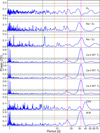 |
Fig. 1 GLS periodogram of serval activity indicators. From top to bottom: Hα λ6562.81A, NaI D1 and D2 λλ5889.9, 5895.92Ǻ, CaII IRT λλλ 8498.02,8542.09,8662.14 Ǻ, CRX, and dLW periodograms. In all panels, the period of the planet candidate at 5.01 d is marked with a vertical dashed green line, and the star-related signals at 8, 16, and 32 days are marked in orange, red, and magenta, respectively. The 10%, 1%, and 0.1% FAPs are marked as horizontal dashed, dash-dotted, and dotted horizontal lines, respectively. The peaks near one day correspond to aliases of the stellar rotation signal, introduced by the daily sampling of ground-based observations. |
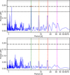 |
Fig. 2 Periodograms with solid vertical lines that indicate the period of the planet candidate at 5 days in green and the star-related periodicities at about 8, 16, and 32 days in orange, red, and magenta, respectively. The 10, 1, and 0.1% FAP levels are marked as horizontal dashed, dash-dotted, and dotted gray lines, respectively. The peaks near one day correspond to aliases of the stellar rotation signal, introduced by the daily sampling of ground-based observations. Top panel: RV data periodogram. The red dot shows the strongest peak signal that is aligned with the orbital period of the planet. Bottom panel: residual periodogram after subtracting the planet and stellar activity signals from the RV data. |
5 Analysis and results
To analyze the photometric and RV data jointly, we employed juliet5 (Espinoza et al. 2019). This is a python package based on other public packages for transit light curve (batman, Kreidberg 2015) and Gaussian Processes (GP; celerite, Foreman-Mackey et al. 2017) modelling that uses nested sampling algorithms (dynesty, Speagle 2020; MultiNest, Feroz et al. 2009; Buchner et al. 2014) to explore the parameter space.
For the photometric and the RV analysis, we performed several fits to determine the model that explained the data better. We started by determining wether the posteriors constrained the prior values and were consistent with the data. In the case of the radial velocities, we plotted the residuals for each performed fit to verify that no signal or additional modulation appeared. Moreover, we examined the completed parameter space and calculate the Bayesian log-evidence (log Z) to facilitate comparisons between models with different numbers of free parameters. According to Trotta (2008), if the difference between two models A and B is ∆ log Z = log ZB - log ZA > 5, then model B is statistically favored over model A with a strong significance. When ∆ log Z ≤ 1, the models are considered statistically indistinguishable, which means that the simpler model with the fewer free parameters is the best model. When ∆ log Z approaches 2.5, however we regarded B to have moderate evidence in its favor compared to A. All the log Z we obtained for the different preformed fits are listed in Table A.1.
For the initial photometric and RV fit, we assumed circular Keplerian orbits to reduce the computation time, that is, we fixed the eccentricity e and argument of periastron (ω) at 0 deg and 90 deg, respectively. In Sect. 5.3, we explore free eccentricity and ω models in the joint fit.
5.1 Photometric modeling
We analyzed the TESS PDC-SAP flux6. We adopted the quadratic limb-darkening law with the (q1, q2) parameterization introduced by Kipping (2013), and we used uniform priors. We considered the uninformative sample (r1, r2) parameterization introduced by Espinoza (2018) to explore the orbital impact parameter (b) and the values of the planet-to-star radius ratio (p = Rp∕R*), where r1 and r2 had uniform priors. We also used the ρ⋆ parameterization for a/R⋆ (Espinoza 2018). We adopted a normal prior based on the stellar properties from Table 1. The dilution factor was fixed to unity, as mentioned in Sect. 2. In addition, we used the same priors to model the MuSCAT2 datasets, but we treated each band separately.
We fit all the available TESS sectors and the two groundbased transits from MuSCAT2. Although the PDC-SAP LC is mainly flat, we included a GP kernel to model possible correlated noise in the data. The selected GP kernel was a celerite (approximate) Matern kernel. The distribution of the priors for the GP amplitude (GPσ) and the GP length scale (GPρ) were carefully chosen to prevent fitting the transit (see Table A.2). We made the same considerations for the MuSCAT2 datasets. The detection shows a significant signal for TESS and for each MuS-CAT2 band, and the fitting models reveal a very clear transit in joint light-curve data. In addition, we explored the TESS LC for other transit events using uniform priors, and avoiding the TOI alerted period value. No transits were found, however. The data returned a lower log Z.
The most relevant planetary parameters obtained with this photometry fit are P ∼ 5.006 d, BJD_TDB - 2457000 (t0) ≈ 2829.762 d, and Rp ∼ 1.84R⊕. The posteriors we obtained are consistent with the TOI alerted values. The inclusion of MuS-CAT2 observations in the photometric modeling significantly improved the transit ephemeris. Ground-based follow-up light curves helped us to refine the orbital period and mid-transit time by extending the observational baseline and reducing the uncertainty between the epoch and the period (e.g. Dragomir et al. 2019; Mallonn et al. 2022). The higher cadence and multiband coverage of MuSCAT2 also provide a better temporal resolution for the transit center, complementing the lower-cadence, longer-baseline TESS data.
5.2 RV modeling
The RV GLS periodogram in Fig. 2 (top panel) shows three relevant signals. The strongest signal lies at the period of the planet detected in the photometric data with a FAP of ∼1%. Therefore, spectroscopic time series confirms the transiting planet. This signal is detected in the RV GLS periodogram, but not in the activity indicator GLS periodograms (see Fig. 1).
The RV GLS periodogram presents two defined additional peaks below the 10% FAP level. These signals are at 8 and 16 days, which are two submultiples of the stellar rotation period at ∼32 days. Moreover, a 32-day signal is detected in some activity indicator periodograms (see Fig. 1 in Sect. 4.2). These signals in the RV time series are therefore likely related to the star and are not the signatures of additional nontransiting planets. In addition, both panels of Fig. 2 show peaks at about one day that correspond to aliases of the stellar rotation signal that are introduced by the daily sampling of the ground-based observation.
We explored different scenarios to model the RV dataset using juliet, and the list of the log Z for the different models is presented in Table A.1. We set a uniform prior from zero to twice the peak-to-peak difference of the data to explore the semiamplitude (K) of the transiting planet. We tested different models to account for the stellar activity-related signals at 8, 16, and 32 days. We considered several GP kernels, but we used the kernel that allowed us to model periodic signals, such as the GP quasi-periodic kernel from celerite (Foreman-Mackey et al. 2017). This kernel was selected because it combines a periodic modulation with a characteristic evolutionary timescale that allowed us to fit the stellar rotation.
The GP quasi-periodic kernel is defined as:
![Mathematical equation: GP_{qp}(\tau) = B \exp\left[ -C \tau - \frac{\sin^2\left( \pi \tau / P_{\mathrm{rot}} \right)}{2L^2} \right] ,](/articles/aa/full_html/2025/08/aa53719-25/aa53719-25-eq5.png)
where τ is the time lag, B is the amplitude of the correlated signal (in m s−1), C controls the exponential decay of active-region signals, and L sets the coherence of the periodic modulation. Prot corresponds to the stellar rotation period, and we adopted a normal prior centered at 8 (half of the first harmonic), 16 (the first harmonic), and 32 days (the stellar rotation period).
The log Z (see Table A.1) significantly favors the planetary models over the nonplanetary ones in the RV-only analyses. This supports a planetary origin independent of photometric data. Of all the explored models, the preferred model consists of a Keplerian for the planetary signal and a GP with the GPProt hyperparameter accounting for the 16 day signal. The GPProt had a normal distribution (see Table A.2) because when we used a uniform distribution, the computation time was high and the posteriors also found the 16-day signal. In addition, the RV residual periodogram (see Fig. 2 bottom panel) shows no significant signals, and the peaks at 8, 16, and 32 days are partially removed using a GPProt of 16 days. Fig. 3 shows the data along with the final RV model. According to the last model we fit in Table A.1, the current RV data do not suggest further nontransiting planets in the system.
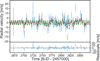 |
Fig. 3 CARMENES radial velocity time series. Top panel: CARMENES data points (blue dots with error bars) along with the best-fit model. The full model is plotted in black, and the Keplerian component is shown in green and the GP model in red. Bottom panel: residuals from the fitted model. |
5.3 Joint fit
In order to better constrain the planet parameters, we jointly fit the photometric and RV time series. In previous sections, we only studied circular orbits for Ross 176 b. After we obtained the best models, we explored eccentric solutions while fitting the photometric and RV datasets simultaneously. The eccentricity and ω were restricted with a constricted distribution, beta and uniform, respectively. The eccentric model converges to planetary parameters consistent with those derived from the photometry and RV analyses alone. This model is preferred over the circular one in terms of log Z (|∆ log Z| ~ 9.3), and its derived parameters have smaller uncertainties.
All the priors, along with the medians and the 68.3% percent credible intervals of the posteriors distributions, are detailed in Table A.2. The planetary parameters derived from the joint fit are gathered in Table 2. The TESS and CARMENES phase-folded transit light curves associated with the joint fit are shown in Fig. 4. The joint-fit model for the MuSCAT2 data is shown in Fig. A.4 in the appendix. The most representative posteriors according to the planetary parameters are shown in Fig. A.5.
6 Discussion
Our photometric and RV analyses confirm a transiting planet around Ross 176. The signal detection is ∼23σ for the radius (Rp = 1.84 ± 0.08 R⊕) and ~5σ for the mass ( ). We derived a mean bulk density for Ross 176b of
  , an eccentricity of e = 0.25 ± 0.04, and an equilibrium temperature (Teq) of
  . A comprehensive list of the planetary parameters is presented in Table 2. The planetary parameters we obtained are consistent with those presented preliminarily in ExoFOP by SPOC. From our analysis of the currently available datasets (see Sect. 5.3), we did not detect any other transiting or nontransiting planet(s) in the system. This suggests that Ross 176 b orbits its host star alone (within our current planet-detection limits).
Planetary parameters of Ross 176 b.
6.1 Is Ross 176b a water-world planet?
The radius and mass of Ross 176 b place it between the superEarth and sub-Neptune regions of the mass-radius diagram (M-R diagram) of all known exoplanets. We filtered the exoplanet catalog from the NASA Exoplanet Archive (Akeson et al. 2013; NASA Exoplanet Archive 2024) and only considered planets with masses and radii determined with a precision better than 20% that orbited K-type stars (Fig. 5).
The planet that is most similar to Ross 176b in the massradius diagram is Wolf 503 b (Rp = 2.043 ± 0.069R⊕, Mp = 6.26 ± 0.70 M⊕,  ; Polanski et al. 2021). Its mass, radius, and mean bulk density are compatible with those of Ross 176 b within 1σ. In the discovery paper of Wolf 503 b, the authors explored different interior composition models and obtained that the planet has an Earth-like core with a substantial water-rich composition (∼45%), which is consistent with the water-world hypothesis and composition (see Fig. 5). Moreover, Wolf 503 b falls within the radius valley described by Fulton & Petigura (2018), as does Ross 176 b. This means that the two planets may have parallel evolutionary and formation histories. Polanski et al. (2021) reported an age of ∼11 Gyr for Wolf 503 b which is much older than Ross 176 b. The two planets are therefore good candidates for testing the X-ray-ultraviolet-driven mass-loss theories (Orell-Miquel et al. 2024).
Another planet similar to Ross 176 b around a K-type stars is HD 40307 b (Tuomi et al. 2013). HD 40307 b is also a waterworld candidate with comparable eccentricities.
6.2 Interior composition of Ross 176b
We used a machine-learning approach to study the interior composition of Ross 176 b with the program ExoMDN7 (Baumeister & Tosi 2023). ExoMDN works with a set of mixture density networks (MDN) and was trained with more than six millions synthetic planet models computed from the code TATOOINE (Baumeister et al. 2020; MacKenzie et al. 2023). The planet training set covered all the planetary masses below 25 M⊕ and Teq between 100–1000 K. The set considered an iron core, a silicate mantle, a water and a high-pressure ice layer, and an He/H atmosphere composition. The planetary input parameters are the mass, the radius, and Teq with their uncertainties, respectively. ExoMDN returns an estimation of the core, the silicate mantle, the water and the gas fraction of the planetary radius (dCore, dMantle, dWater, and dGas, respectively), and the mass (wCore, wMantle, wWater, and wGas, respectively).
The interior composition predicted by ExoMDN for Ross 176 b is shown in Fig. 6. The derived water fraction of Ross 176b is 14% in mass fraction, which is higher than that of the Earth (Fig. 5). Although the central value of the water mass fraction is lower than the 50% predicted for the water-world classification (Luque & Pallé 2022) when we consider the upper uncertainty, it is consistent at ~1σ with this classification (see the right panel in Fig. 6). The 1σ lower uncertainty might be consistent with zero as well, however, which highlights the degeneracies in internal structure inferences from mass-radius data alone (Rogers & Seager 2010; Zeng et al. 2019; Luo et al. 2024). The gas fraction is negligible in mass, and it only represents about 10% in radius. We note, however, that ExoMDN assumes a layered internal structure, which may not be the case for water worlds and sub-Neptunes in general (see Dorn & Lichtenberg 2021; Vazan et al. 2022; Luo et al. 2024; Rogers et al. 2024). Thus, according to the previous analysis (Sects. 6.1 and 6.2), Ross 176b is a promising water-world candidate planet.
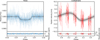 |
Fig. 4 Phase-folded joint fit of Ross 176 b. Left panel: phase-folded transits from TESS (blue points) with the joint-fit model (black line). Right panel: phase-folded RV data from CARMENES (red points), with the joint-fit model (black line), and the 1σ, 2σ, and 3σ confidence intervals for the model (shaded gray areas). The two panels show the binned data for clarity (white points), the residuals from the fit at the bottom, and the error bars include the instrumental jitter term added in quadrature. The LC data are binned by ∼30 mins, and the RV data are binned by two points every 0.2 phase. |
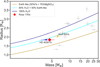 |
Fig. 5 Mass and radius diagram for Ross 176 b. There are two world composition models from Zeng et al. 2019: The brown model is an Earth-like planet (30% Fe + 70% MgSiO3), the blue model is a waterworld planet (50% H2O + 50% Earth-like), the navy blue line is a full water-world planet (100% H2O) with a Teq of 700 K. The gray dots show confirmed exoplanets from the NASA exoplanet archive filtered with a mass and radius precision better than 20% that orbit K-type stars in April 2025. |
6.3 Prospective atmosphere characterization with JWST
We adopted the metrics proposed by Kempton et al. (2018) to qualitatively assess whether Ross 176 b is suitable for an atmospheric characterization. The transmission spectroscopy metric (TSM) is 52 , and the emission spectroscopy metric (ESM) is 4.0±0.4. These two metrics are slightly below the recommended thresholds of TSM≳90 for small sub-Neptunes (1.5 R⊕ < Rp < 2.75 R⊕), and ESM≳7.5. The ESM was designed for terrestrial planets (Rp < 1.5 R⊕), however, and it is proportional to
  , which further weakens the candidacy of Ross 176b for emission spectroscopy observations. It is also worth noting that the TSM and ESM rank planets solely based on the predicted strength of their atmospheric signals, regardless of scientific interest. Ross 176b is one of the highest TSM planets orbiting a K dwarf with a precise mass measurement (<20%). Most of the other top-ranked candidates were discovered around M dwarfs. It might therefore be a key object for probing planetary formation and evolution under different conditions, especially because the extreme-XUV irradiation from K stars is far lower than that of M host stars. Thet the TSM and ESM values are slightly lower than the above thresholds does not exclude the feasibility of atmospheric studies of Ross 176 b.
We simulated JWST transmission spectra for atmospheric models consistent with the physical properties of Ross 176 b, as they would be observed with the James Webb Space Telescope (JWST; Gardner et al. 2006). We explored a range of atmospheric scenarios, including H/He-dominated compositions with one and one hundred times the solar metallicity, both clear and hazy, as well as a pure water-vapor atmosphere. Synthetic transmission spectra were generated using TauREx 3 (Waldmann et al. 2015; Al-Refaie et al. 2021). For the H/He atmospheres, we assumed atmospheric chemical equilibrium (Agúndez et al. 2012), including collisionally induced absorption by H2–H2 and H2–He (Abel et al. 2011, 2012; Fletcher et al. 2018), and Rayleigh scattering. The haze was modeled using the Mie scattering theory, following the formalism of Lee et al. (2013), with a particle size of α = 0.05 µm, a mixing ratio of χc = 10−12, and an extinction coefficient of Q0 = 40. Although these selected cases may not capture all possible scenarios or the full complexity of a real atmosphere (e.g., Mishchenko et al. 1996; Ma et al. 2023), they provide a practical set of benchmark models for evaluation purposes (Orell-Miquel et al. 2023; Goffo et al. 2024). We note that planetary formation theories predict significant metal enrichment in mini-Neptune atmospheres (Fortney et al. 2013; Thorngren et al. 2016). Microphysical models of cloud formation consistently indicate a high degree of potential haziness in temperate planetary atmospheres (Gao & Zhang 2020; Ohno & Tanaka 2021; Yu et al. 2021).
We used ExoTETHyS (Morello et al. 2021) to simulate the corresponding JWST spectra for the NIRISS-SOSS (0.6–2.8 µm), NIRSpec-G395H (2.88–5.20 µm), and MIRI-LRS (5–12 µm) instrumental setups. The ExoTETHyS software has been benchmarked against the Exoplanet Characterization Toolkit (ExoCTK, Bourque et al. 2021) and PandExo (Batalha et al. 2017) in previous studies (Murgas et al. 2021; Espinoza et al. 2022; Luque et al. 2022a,b; Chaturvedi et al. 2022; Lillo-Box et al. 2023; Orell-Miquel et al. 2023; Palle et al. 2023; Goffo et al. 2024). As usual, we applied a conservative 20% increase to the error estimates. Following the recommendations in recent JWST data synthesis papers, we selected the wavelength bin sizes based on a spectral resolution of R ∼ 100 for NIRISS and NIRSpec (Carter et al. 2024), and a constant bin size of 0.25 µm for MIRI-LRS observations (Powell et al. 2024).
Fig. 7 presents the synthetic transmission spectra for the atmospheric models described above. The H/He atmosphere models show prominent H2O and CH4 absorption features that reach several hundred parts per million (ppm) for the one time solar metallicity composition. In the one hundred time solar metallicity scenarios, the strongest feature (>100 ppm) would be due to CO2 at 4.3 µm, which is detectable with NIRSpec-G395H. Haze mostly affects the NIRISS-SOSS wavelength range. The steam H2 O atmosphere has much smaller absorption features of ≲30 ppm. The predicted error bars for a single transit observation are 26–101 ppm (mean error 43 ppm) for NIRISS-SOSS, 31–82 ppm (mean error 46 ppm) for NIRSpec-G395H, and 40–76 ppm (mean error 54 ppm) for MIRI-LRS. Our simulations suggest that a single transit observation may be sufficient to detect an H/He atmosphere. In the water-world scenario, the atmospheric signal would be more challenging to detect even when many transit spectra were stacked. Nonetheless, a flat transmission spectrum may be useful to rule out the mini-Neptune hypothesis, leaving the water-world as the only option consistent with the mass and radius measurements (e.g., Damiano et al. 2024).
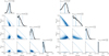 |
Fig. 6 Interior composition simulation, of Ross 176 b that shows the core, the mantle, the water, and the gas fraction for the planet formation. Left panel: radius fraction composition. Right panel: mass fraction composition. |
6.4 Implication of the orbital eccentricity
We explored the potential implications of an eccentric orbit for Ross 176 b and how this might change our understanding of the system formation and evolution. Ross 176b is part of the population of small planets with short orbital periods. The members of this group frequently exhibit mean eccentricities ranging from ∼0.15–0.20, particularly those with orbital periods shorter than ∼10 days (MacDonald 1964). This trend toward moderate eccentricities among close-in Neptunes has also been highlighted by Correia et al. (2020).
The eccentricity distribution of Neptune planets shows a distinct pattern in the period–eccentricity diagram compared to other planet types (see Fig. 1 in Correia et al. 2020). While giant planets generally display increasing eccentricities beyond orbital periods of 5 days, smaller planets (R < 3 Re) tend to maintain low eccentricities. When we understand where Ross 176 b falls within this framework, we may shed more light on its dynamical history.
We reproduced the bottom panel of Fig. 1 in Correia et al. (2020) using the NASA Exoplanet Archive data. We filtered the exoplanet catalog considering only planets with Rp between 1 and 3 Re, an orbital period in the range 1 < Porb < 100 days, and eccentricities determined with a precision better than 70%. We restricted our planet selection to those orbiting M- and K-type stars (see Fig. 8).
The eccentricity of Ross 176b is consistent with the eccentricities of other short-period small planets orbiting late-type stars. The slightly eccentric orbit might be due to the interaction of Ross 176b with a long orbital period planet (Raymond et al. 2011), although our analysis does not suggest the presence of further companions.
The period of Ross 176 b’s prevent us from covering the full orbital phases of the planet from a single site in one season (see Fig. 4 right panel). Further RV observations from a different location will help us to sample the missing phases and fully constrain the eccentricity of Ross 176 b.
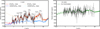 |
Fig. 7 Synthetic atmospheric transmission spectra of Ross 176 b. Left: Fiducial models for clear or hazy H/He atmospheres with scaled solar abundances. Right: model for a steam H2O atmosphere. Simulated measurements with error bars are shown for the observation of one (left) or ten (right) transits with JWST NIRISS-SOSS, NIRSpec-G395H, and MIRI-LRS configurations. |
7 Conclusions
We presented the discovery and characterization of Ross 176 b, a small planet transiting a late K-type star observed with TESS, MuSCAT2, and CARMENES. This planet is a candidate waterworld. Ross 176b is a planet between the super-Earth and subNeptune regimes inside the radius gap, with a planetary radius and mass of Rp ~ 1.8 R⊕ and Mp ~ 4.6 M⊕. This planet increases the small population of planets with well-determined masses (precision better than 20%) around K-type stars. Ross 176b is a hot planet with a Teq = 682 K, which is high enough to discard the possibility that it is a habitable world. Furthermore, Ross 176b is the second exoplanet with a higher instellation orbiting a K7 V star (TOI-1130 b is the planet with the highest instellation, Sp = 78.10 ± 5.55; Korth et al. 2023).
We explored the planet composition with ExoMDN, a machine-learning approach that assumes a layered internal structure. According to our results, the inferred water radius fraction is compatible with a 50% water composition by mass, as expected for the water-world population, although the data also allow a composition with little to no water content.
Ross 176 b is a suitable candidate for further atmospheric studies with the JWST, which could break the interior structure degeneracies. Atmospheric studies are also key to expanding our knowledge of planetary compositions by providing information on the processes involved in the evolution and formation of sub-Neptunes.
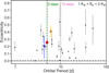 |
Fig. 8 Eccentricity-orbital period diagram for planets with Rp = 1–3 R⊕. Ross 176 b, HD 40307 b, and Wolf 503 b are overplotted in red, blue, and orange, respectively, following the same criteria as in Fig. 5. The precision of the eccentricities and the orbital periods of the planets is better than 70 and 10%, respectively. The vertical green line shows the period of 5 days, which is the upper limit for smaller planets to tend to maintain low eccentricities. On other hand, the vertical pink line shows the period of planets with non-neligible eccentricities (Correia et al. 2020). |
Data availability
The MuSCAT2 photometric data, radial velocity, and activity indices are available at the CDS via https://cdsarc.cds.unistra.fr/viz-bin/cat/J/A+A/700/A216
Acknowledgements
This paper includes data collected with the TESS mission, obtained from the MAST data archive at the Space Telescope Science Institute (STScI). Funding for the TESS mission is provided by the NASA Explorer Program. STScI is operated by the Association of Universities for Research in Astronomy, Inc., under NASA contract NAS 5–26555. We acknowledge the use of TESS Alert data, which is currently in a beta test phase, from pipelines at the TESS Science Office and at the TESS Science Processing Operations Center. We acknowledge the use of public TESS Alert data from pipelines at the TESS Science Office and at the TESS Science Processing Operations Center. This research has made use of the Exoplanet Follow-up Observation Program website, which is operated by the California Institute of Technology, under contract with the National Aeronautics and Space Administration under the Exoplanet Exploration Program. Resources supporting this work were provided by the NASA High-End Computing (HEC) Program through the NASA Advanced Supercomputing (NAS) Division at Ames Research Center for the production of the SPOC data products. This paper includes data collected by the TESS mission, which are publicly available from the Mikulski Archive for Space Telescopes (MAST). CARMENES is an instrument at the Centro Astronómico Hispano en Andalucía (CAHA) at Calar Alto (Almería, Spain), operated jointly by the Junta de Andalucía and the Instituto de Astrofísica de Andalucía (CSIC). The authors wish to express their sincere thanks to all members of the Calar Alto staff for their expert support of the instrument and telescope operation. CARMENES was funded by the Max-Planck-Gesellschaft (MPG), the Consejo Superior de Investigaciones Científicas (CSIC), the Ministerio de Economía y Competitividad (MINECO) and the European Regional Development Fund (ERDF) through projects FICTS-2011-02, ICTS-2017-07-CAHA-4, and CAHA16-CE-3978, and the members of the CARMENES Consortium (Max-Planck-Institut für Astronomie, Instituto de Astrofísica de Andalucía, Lan-dessternwarte Königstuhl, Institut de Ciències de l’Espai, Institut für Astrophysik Göttingen, Universidad Complutense de Madrid, Thüringer Landessternwarte Tautenburg, Instituto de Astrofísica de Canarias, Hamburger Sternwarte, Centro de Astrobiología and Centro Astronómico Hispano-Alemán), with additional contributions by the MINECO, the Deutsche Forschungsgemeinschaft (DFG) through the Major Research Instrumentation Programme and Research Unit FOR2544 “Blue Planets around Red Stars”, the Klaus Tschira Stiftung, the states of Baden-Württemberg and Niedersachsen, and by the Junta de Andalucía. This paper is based on observations made with the MuSCAT2 instrument, developed by ABC, at Telescopio Carlos Sánchez operated on the island of Tenerife by the IAC in the Spanish Observatorio del Teide. We acknowledge financial support from the Agencia Estatal de Investigación (AEI/10.13039/501100011033) of the Ministerio de Ciencia e Innovación and the ERDF “A way of making Europe” through projects PID2023-150468NB-I00, PID2022-137241NB-C4[1:4], PID2021-125627OB-C31, PID2019-107061GB-C61, RYC2022-037854-I, RYC2021-031798-I, RYC2021-031640-I, CNS2023-144309, and the Centre of Excellence “Severo Ochoa” and “María de Maeztu” awards to the Instituto de Astrofísica de Canarias (CEX2019-000920-S), Instituto de Astrofísica de Andalucía (CEX2021-001131-S) and Institut de Ciències de l’Espai (CEX2020-001058-M). This work was also funded by the Generalitat de Catalunya/CERCA programme; the Universidad de la Laguna and the Ministerio de Ciencia, Innovación y Universidades; the Bulgarian National Science Fund through program “VIHREN-2021” project No. KP-06-DV/5; Japan Society for the Promotion of Science via JSPS KAKENHI Grant no. JP24H00017, JP24K00689, JP24K17083, JSPS Grant-in-Aid for JSPS Fellows Grant no. JP24KJ0241, and JSPS Bilateral Program no. JPJSBP120249910; NASA through the NASA Hubble Fellowship grant #HST-HF2-51559.001-A awarded by the Space Telescope Science Institute, which is operated by the Association of Universities for Research in Astronomy, Inc., for NASA, under contract NAS5-26555; and the project “Tecnologías avanzadas para la exploración de universo y sus componentes” (PR47/21 TAU) funded by Comunidad de Madrid, by the Recovery, Transformation and Resilience Plan from the Spanish State, and by NextGen-erationEU from the European Union through the Recovery and Resilience Facility. The results reported herein benefitted from collaborations and/or information exchange within NASA’s Nexus for Exoplanet System Science (NExSS) research coordination network sponsored by NASA’s Science Mission Directorate under Agreement No. 80NSSC21K0593 for the program “Alien Earths”. This work made use of tpfplotter by J. Lillo-Box (publicly available in www.github.com/jlillo/tpfplotter), which also made use of the python packages astropy, lightkurve, matplotlib and numpy.
Appendix A Additional figures and tables
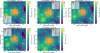 |
Fig. A.1 TESS target pixel file images of Ross 176 (TIC 193336820) observed in sectors 14, 15, 41, 55, and 56 (made with tpfplotter). The pixels highlighted in red show the aperture used by TESS to obtain the photometry. The electron counts are color-coded. The positions and sizes of the red circles represent the positions and TESS magnitudes of nearby stars, respectively. Ross 176 is marked with a cross (×) and labelled with #1. |
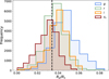 |
Fig. A.2 Planet-to-star radius distribution for all MuSCAT2 bands (g′, r′, i′, and z′). The dashed vertical line corresponds to the center of the Planet-to-star radius distribution provided by TESS. |
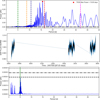 |
Fig. A.3 Periodicity analysis of the TESS SAP flux of Ross 176. The 10%, 1% and 0.1% FAP levels in the GLS panels are marked as horizontal dashed, dash-dotted and dotted gray lines, respectively. Top panel: GLS periodogram for the SAP data, following the same color criteria for the vertical lines with an exception of the new dark blue line which points out the second harmonic of the stellar rotation period (Prot)/3 ∼ 10-11 days. Mid panel: median-normalized SAP LC (blue data points) along with the GP celerite quasi-periodic kernel model with a GP_Prot around 32 days (black line). Bottom panel: GLS periodogram of the SAP light curve residuals after subtracting the GP model from the photometric dataset. The period of Ross 176b at 5.01 d (green line) and the FAP lines are also represented. |
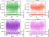 |
Fig. A.4 Phase-folded transit light curves of Ross 176 b in all MuSCAT2 bands (g′, r′, i′, and z′s). All of them have the same joint fit model for each filter. Each panel has attached the residuals at the bottom. The data is grouped by the binning approximately every 24 minutes. |
Bayesian log-evicence (log Z) and the Ross 176 b semi-amplitude (K) for the studied RV models.
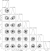 |
Fig. A.5 Posteriors corner plot from the joint fit. We choose the most representative posteriors according to the derived planetary parameters. |
Priors, along with medians and 68.3% percent credible intervals of the posterior distributions of the model parameters, as derived from the joint fit analysis performed with juliet for Ross 176 b.
References
- Abel, M., Frommhold, L., Li, X., & Hunt, K. L. C. 2011, J. Phys. Chem. A, 115, 6805 [NASA ADS] [CrossRef] [Google Scholar]
- Abel, M., Frommhold, L., Li, X., & Hunt, K. L. C. 2012, J. Chem. Phys., 136, 044319 [NASA ADS] [CrossRef] [Google Scholar]
- Agúndez, M., Venot, O., Iro, N., et al. 2012, A&A, 548, A73 [NASA ADS] [CrossRef] [EDP Sciences] [Google Scholar]
- Akeson, R. L., Chen, X., Ciardi, D., et al. 2013, PASP, 125, 989 [Google Scholar]
- Al-Refaie, A. F., Changeat, Q., Waldmann, I. P., & Tinetti, G. 2021, ApJ, 917, 37 [NASA ADS] [CrossRef] [Google Scholar]
- Aller, A., Lillo-Box, J., Jones, D., Miranda, L. F., & Barceló Forteza, S. 2020, A&A, 635, A128 [NASA ADS] [CrossRef] [EDP Sciences] [Google Scholar]
- Angus, R., Aigrain, S., Foreman-Mackey, D., & McQuillan, A. 2015, MNRAS, 450, 1787 [Google Scholar]
- Barnes, S. A. 2007, ApJ, 669, 1167 [Google Scholar]
- Batalha, N. E., Mandell, A., Pontoppidan, K., et al. 2017, PASP, 129, 064501 [Google Scholar]
- Baumeister, P., & Tosi, N. 2023, A&A, 676, A106 [NASA ADS] [CrossRef] [EDP Sciences] [Google Scholar]
- Baumeister, P., Padovan, S., Tosi, N., et al. 2020, ApJ, 889, 42 [Google Scholar]
- Bidelman, W. P. 1985, ApJS, 59, 197 [Google Scholar]
- Borucki, W. J., Agol, E., Fressin, F., et al. 2013, Science, 340, 587 [NASA ADS] [CrossRef] [Google Scholar]
- Bouma, L. G., Palumbo, E. K., & Hillenbrand, L. A. 2023, ApJ, 947, L3 [NASA ADS] [CrossRef] [Google Scholar]
- Bourque, M., Espinoza, N., Filippazzo, J., et al. 2021, https://doi.org/10.5281/zenodo.4556063 [Google Scholar]
- Buchner, J., Georgakakis, A., Nandra, K., et al. 2014, A&A, 564, A125 [NASA ADS] [CrossRef] [EDP Sciences] [Google Scholar]
- Caballero, J. A., Cortés-Contreras, M., Alonso-Floriano, F. J., et al. 2016a, in 19th Cambridge Workshop on Cool Stars, Stellar Systems, and the Sun (CS19), 148 [Google Scholar]
- Caballero, J. A., Guàrdia, J., López del Fresno, M., et al. 2016b, SPIE Conf. Ser., 9910, 99100E [Google Scholar]
- Carter, A. L., May, E. M., Espinoza, N., et al. 2024, Nat. Astron., submitted [arXiv:2407.13893] [Google Scholar]
- Chaturvedi, P., Bluhm, P., Nagel, E., et al. 2022, A&A, 666, A155 [NASA ADS] [CrossRef] [EDP Sciences] [Google Scholar]
- Cifuentes, C., Caballero, J. A., Cortés-Contreras, M., et al. 2020, A&A, 642, A115 [NASA ADS] [CrossRef] [EDP Sciences] [Google Scholar]
- Correia, A. C. M., Bourrier, V., & Delisle, J. B. 2020, A&A, 635, A37 [NASA ADS] [CrossRef] [EDP Sciences] [Google Scholar]
- Cortés-Contreras, M., Caballero, J. A., Montes, D., et al. 2024, A&A, 692, A206 [NASA ADS] [CrossRef] [EDP Sciences] [Google Scholar]
- Cutri, R. M., Wright, E. L., Conrow, T., et al. 2021, VizieR Online Data Catalog: AllWISE Data Release (Cutri+ 2013), VizieR On-line Data Catalog: II/328 [Google Scholar]
- Damiano, M., Bello-Arufe, A., Yang, J., & Hu, R. 2024, ApJ, 968, L22 [Google Scholar]
- Dorn, C., & Lichtenberg, T. 2021, ApJ, 922, L4 [NASA ADS] [CrossRef] [Google Scholar]
- Dragomir, D., Teske, J., Günther, M. N., et al. 2019, ApJ, 875, L7 [Google Scholar]
- Espinoza, N. 2018, RNAAS, 2, 209 [Google Scholar]
- Espinoza, N., Kossakowski, D., & Brahm, R. 2019, MNRAS, 490, 2262 [Google Scholar]
- Espinoza, N., Pallé, E., Kemmer, J., et al. 2022, AJ, 163, 133 [NASA ADS] [CrossRef] [Google Scholar]
- Feroz, F., Hobson, M. P., & Bridges, M. 2009, MNRAS, 398, 1601 [NASA ADS] [CrossRef] [Google Scholar]
- Fletcher, L. N., Gustafsson, M., & Orton, G. S. 2018, ApJS, 235, 24 [NASA ADS] [CrossRef] [Google Scholar]
- Foreman-Mackey, D., Agol, E., Angus, R., & Ambikasaran, S. 2017, AJ, 154, 220 [NASA ADS] [CrossRef] [Google Scholar]
- Fortney, J. J., Mordasini, C., Nettelmann, N., et al. 2013, ApJ, 775, 80 [Google Scholar]
- Fulton, B. J., & Petigura, E. A. 2018, AJ, 156, 264 [Google Scholar]
- Gaia Collaboration 2020, VizieR Online Data Catalog: I/350 [Google Scholar]
- Gaia Collaboration (Smart, R. L., et al.) 2021, A&A, 649, A6 [EDP Sciences] [Google Scholar]
- Gaia Collaboration (Vallenari, A., et al.) 2023, A&A, 674, A1 [NASA ADS] [CrossRef] [EDP Sciences] [Google Scholar]
- Gao, P., & Zhang, X. 2020, ApJ, 890, 93 [Google Scholar]
- Gardner, J. P., Mather, J. C., Clampin, M., et al. 2006, Space Sci. Rev., 123, 485 [Google Scholar]
- Goffo, E., Chaturvedi, P., Murgas, F., et al. 2024, A&A, 685, A147 [NASA ADS] [CrossRef] [EDP Sciences] [Google Scholar]
- Guerrero, N. M., Seager, S., Huang, C. X., et al. 2021, ApJS, 254, 39 [NASA ADS] [CrossRef] [Google Scholar]
- Henden, A. A., Templeton, M., Terrell, D., et al. 2016, VizieR Online Data Catalog: AAVSO Photometric All Sky Survey (APASS) DR9 (Henden+, 2016), VizieR On-line Data Catalog: II/336 [Google Scholar]
- Høg, E., Fabricius, C., Makarov, V. V., et al. 2000, A&A, 355, L27 [Google Scholar]
- Huang, C. X., Vanderburg, A., Pál, A., et al. 2020a, Res. Notes Am. Astron. Soc., 4, 204 [Google Scholar]
- Huang, C. X., Vanderburg, A., Pál, A., et al. 2020b, Res. Notes Am. Astron. Soc., 4, 206 [Google Scholar]
- Jenkins, J. M., Twicken, J. D., McCauliff, S., et al. 2016, SPIE, 9913, 99133E [NASA ADS] [Google Scholar]
- Kausch, W., Noll, S., Smette, A., et al. 2015, A&A, 576, A78 [NASA ADS] [CrossRef] [EDP Sciences] [Google Scholar]
- Kempton, E. M. R., Bean, J. L., Louie, D. R., et al. 2018, PASP, 130, 114401 [Google Scholar]
- Kipping, D. M. 2013, MNRAS, 435, 2152 [Google Scholar]
- Kite, E. S., & Ford, E. B. 2018, ApJ, 864, 75 [Google Scholar]
- Korth, J., Gandolfi, D., Šubjak, J., et al. 2023, A&A, 675, A115 [NASA ADS] [CrossRef] [EDP Sciences] [Google Scholar]
- Kreidberg, L. 2015, PASP, 127, 1161 [Google Scholar]
- Kuzuhara, M., Fukui, A., Livingston, J. H., et al. 2024, ApJ, 967, L21 [Google Scholar]
- Lacedelli, G., Pallé, E., Luque, R., et al. 2024, A&A, 692, A238 [NASA ADS] [CrossRef] [EDP Sciences] [Google Scholar]
- Lee, S. G. 1984, AJ, 89, 702 [NASA ADS] [CrossRef] [Google Scholar]
- Lee, J.-M., Heng, K., & Irwin, P. G. J. 2013, ApJ, 778, 97 [Google Scholar]
- Lépine, S., & Shara, M. M. 2005, AJ, 129, 1483 [Google Scholar]
- Lillo-Box, J., Santos, N. C., Santerne, A., et al. 2022, A&A, 667, A102 [NASA ADS] [CrossRef] [EDP Sciences] [Google Scholar]
- Lillo-Box, J., Gandolfi, D., Armstrong, D. J., et al. 2023, A&A, 669, A109 [NASA ADS] [CrossRef] [EDP Sciences] [Google Scholar]
- Lingam, M., & Loeb, A. 2017, ApJ, 846, L21 [Google Scholar]
- Lingam, M., & Loeb, A. 2019, J. Cosmol. Astropart. Phys., 5, 020 [Google Scholar]
- Luo, H., Dorn, C., & Deng, J. 2024, Nat. Astron., 8, 1399 [Google Scholar]
- Luque, R., & Pallé, E. 2022, Science, 377, 1211 [NASA ADS] [CrossRef] [Google Scholar]
- Luque, R., Fulton, B. J., Kunimoto, M., et al. 2022a, A&A, 664, A199 [NASA ADS] [CrossRef] [EDP Sciences] [Google Scholar]
- Luque, R., Nowak, G., Hirano, T., et al. 2022b, A&A, 666, A154 [NASA ADS] [CrossRef] [EDP Sciences] [Google Scholar]
- Luyten, W. J. 1957, A catalogue of 9867 stars in the Southern Hemisphere with proper motions exceeding 0.”2 annually (Minneapolis: Lund Press) [Google Scholar]
- Ma, S., Ito, Y., Al-Refaie, A. F., et al. 2023, ApJ, 957, 104 [NASA ADS] [CrossRef] [Google Scholar]
- MacDonald, G. J. F. 1964, Rev. Geophys. Space Phys., 2, 467 [Google Scholar]
- MacKenzie, J., Grenfell, J. L., Baumeister, P., et al. 2023, A&A, 671, A65 [NASA ADS] [CrossRef] [EDP Sciences] [Google Scholar]
- Mallonn, M., Poppenhaeger, K., Granzer, T., Weber, M., & Strassmeier, K. G. 2022, A&A, 657, A102 [NASA ADS] [CrossRef] [EDP Sciences] [Google Scholar]
- Mallorquín, M., Béjar, V. J. S., Lodieu, N., et al. 2024, A&A, 689, A132 [NASA ADS] [CrossRef] [EDP Sciences] [Google Scholar]
- Mamajek, E. E., & Hillenbrand, L. A. 2008, ApJ, 687, 1264 [Google Scholar]
- Marfil, E., Tabernero, H. M., Montes, D., et al. 2021, VizieR Online Data Catalog: J/A+A/656/A162 [Google Scholar]
- Mishchenko, M. I., Travis, L. D., & Mackowski, D. W. 1996, J. Quant. Spec. Radiat. Transf., 55, 535 [NASA ADS] [CrossRef] [Google Scholar]
- Morello, G., Zingales, T., Martin-Lagarde, M., Gastaud, R., & Lagage, P.-O. 2021, AJ, 161, 174 [NASA ADS] [CrossRef] [Google Scholar]
- Morris, R. L., Twicken, J. D., Smith, J. e. C., et al. 2020, Kepler Data Processing Handbook: Photometric Analysis, Kepler Science Document KSCI-19081-003, ed. Jon M. Jenkins (USA: NASA), 6 [Google Scholar]
- Murgas, F., Astudillo-Defru, N., Bonfils, X., et al. 2021, A&A, 653, A60 [NASA ADS] [CrossRef] [EDP Sciences] [Google Scholar]
- Murgas, F., Pallé, E., Orell-Miquel, J., et al. 2024, A&A, 684, A83 [NASA ADS] [CrossRef] [EDP Sciences] [Google Scholar]
- Nagel, E., Czesla, S., Kaminski, A., et al. 2023, A&A, 680, A73 [NASA ADS] [CrossRef] [EDP Sciences] [Google Scholar]
- Narita, N., Fukui, A., Kusakabe, N., et al. 2019, J. Astron. Telesc. Instrum. Syst., 5, 015001 [NASA ADS] [Google Scholar]
- NASA Exoplanet Archive. 2024, Planetary Systems (NExScI-Caltech/IPAC) [Google Scholar]
- Ohno, K., & Tanaka, Y. A. 2021, ApJ, 920, 124 [NASA ADS] [CrossRef] [Google Scholar]
- Orell-Miquel, J., Nowak, G., Murgas, F., et al. 2023, A&A, 669, A40 [NASA ADS] [CrossRef] [EDP Sciences] [Google Scholar]
- Orell-Miquel, J., Murgas, F., Pallé, E., et al. 2024, A&A, 689, A179 [NASA ADS] [CrossRef] [EDP Sciences] [Google Scholar]
- Palle, E., Orell-Miquel, J., Brady, M., et al. 2023, A&A, 678, A80 [NASA ADS] [CrossRef] [EDP Sciences] [Google Scholar]
- Parviainen, H. 2022, Astrophysics Source Code Library [record ascl:2207.013] [Google Scholar]
- Parviainen, H., Tingley, B., Deeg, H. J., et al. 2019, A&A, 630, A89 [NASA ADS] [CrossRef] [EDP Sciences] [Google Scholar]
- Parviainen, H., Palle, E., Zapatero-Osorio, M. R., et al. 2020, A&A, 633, A28 [NASA ADS] [CrossRef] [EDP Sciences] [Google Scholar]
- Passegger, V. M., Reiners, A., Jeffers, S. V., et al. 2018, A&A, 615, A6 [NASA ADS] [CrossRef] [EDP Sciences] [Google Scholar]
- Polanski, A. S., Crossfield, I. J. M., Burt, J. A., et al. 2021, AJ, 162, 238 [NASA ADS] [CrossRef] [Google Scholar]
- Powell, D., Feinstein, A. D., Lee, E. K. H., et al. 2024, Nature, 626, 979 [NASA ADS] [CrossRef] [Google Scholar]
- Quirrenbach, A., Amado, P. J., Caballero, J. A., et al. 2014, SPIE Conf. Ser., 9147, 91471F [Google Scholar]
- Raymond, S. N., Armitage, P. J., Moro-Martín, A., et al. 2011, A&A, 530, A62 [NASA ADS] [CrossRef] [EDP Sciences] [Google Scholar]
- Reiners, A., Zechmeister, M., Caballero, J. A., et al. 2018, A&A, 612, A49 [NASA ADS] [CrossRef] [EDP Sciences] [Google Scholar]
- Richey-Yowell, T., Shkolnik, E. L., Loyd, R. O. P., et al. 2022, ApJ, 929, 169 [Google Scholar]
- Ricker, G. R., Winn, J. N., Vanderspek, R., et al. 2015, J. Astron. Telesc. Instrum. Syst., 1, 014003 [Google Scholar]
- Rimmer, P. B., Xu, J., Thompson, S. J., et al. 2018, Sci. Adv., 4, eaar3302 [Google Scholar]
- Rogers, L. A., & Seager, S. 2010, ApJ, 716, 1208 [NASA ADS] [CrossRef] [Google Scholar]
- Rogers, J. G., Schlichting, H. E., & Young, E. D. 2024, ApJ, 970, 47 [NASA ADS] [CrossRef] [Google Scholar]
- Ross, F. E. 1926, AJ, 36, 172 [Google Scholar]
- Ruh, H. L., Zechmeister, M., Reiners, A., et al. 2024, A&A, 692, A138 [NASA ADS] [CrossRef] [EDP Sciences] [Google Scholar]
- Schweitzer, A., Passegger, V. M., Cifuentes, C., et al. 2019, A&A, 625, A68 [NASA ADS] [CrossRef] [EDP Sciences] [Google Scholar]
- Segura, A., Kasting, J., Meadows, V., et al. 2005, Astrobiology, 5, 706 [Google Scholar]
- Skrutskie, M. F., Cutri, R. M., Stiening, R., et al. 2006, AJ, 131, 1163 [NASA ADS] [CrossRef] [Google Scholar]
- Smette, A., Sana, H., Noll, S., et al. 2015, A&A, 576, A77 [NASA ADS] [CrossRef] [EDP Sciences] [Google Scholar]
- Smith, J. C., Stumpe, M. C., Van Cleve, J. E., et al. 2012, PASP, 124, 1000 [Google Scholar]
- Speagle, J. S. 2020, MNRAS, 493, 3132 [Google Scholar]
- Stassun, K. G., Oelkers, R. J., Pepper, J., et al. 2018, AJ, 156, 102 [Google Scholar]
- Stassun, K. G., Oelkers, R. J., Paegert, M., et al. 2019, AJ, 158, 138 [Google Scholar]
- Stumpe, M. C., Smith, J. C., Van Cleve, J. E., et al. 2012, PASP, 124, 985 [Google Scholar]
- Stumpe, M. C., Smith, J. C., Catanzarite, J. H., et al. 2014, PASP, 126, 100 [Google Scholar]
- Tabernero, H. M., Marfil, E., Montes, D., & González Hernández, J. I. 2022, A&A, 657, A66 [NASA ADS] [CrossRef] [EDP Sciences] [Google Scholar]
- Thorngren, D. P., Fortney, J. J., Murray-Clay, R. A., & Lopez, E. D. 2016, ApJ, 831, 64 [NASA ADS] [CrossRef] [Google Scholar]
- Trifonov, T., Tal-Or, L., Zechmeister, M., et al. 2020, A&A, 636, A74 [NASA ADS] [CrossRef] [EDP Sciences] [Google Scholar]
- Trotta, R. 2008, Contemp. Phys., 49, 71 [Google Scholar]
- Tuomi, M., Anglada-Escudé, G., Gerlach, E., et al. 2013, A&A, 549, A48 [NASA ADS] [CrossRef] [EDP Sciences] [Google Scholar]
- van Altena, W. F., Lee, J. T., & Hoffleit, E. D. 1995, The general catalogue of trigonometric [stellar] parallaxes (New Haven, CT: Yale University Observatory) [Google Scholar]
- Vazan, A., Sari, R., & Kessel, R. 2022, ApJ, 926, 150 [NASA ADS] [CrossRef] [Google Scholar]
- Waldmann, I. P., Tinetti, G., Rocchetto, M., et al. 2015, ApJ, 802, 107 [CrossRef] [Google Scholar]
- Weis, E. W. 1988, AJ, 96, 1710 [Google Scholar]
- Yu, X., He, C., Zhang, X., et al. 2021, Nat. Astron., 5, 822 [NASA ADS] [CrossRef] [Google Scholar]
- Zechmeister, M., & Kürster, M. 2009, A&A, 496, 577 [CrossRef] [EDP Sciences] [Google Scholar]
- Zechmeister, M., Reiners, A., Amado, P. J., et al. 2018, A&A, 609, A12 [NASA ADS] [CrossRef] [EDP Sciences] [Google Scholar]
- Zeng, L., Jacobsen, S. B., Sasselov, D. D., et al. 2019, Proc. Natl. Acad. Sci., 116, 9723 [Google Scholar]
The PDC algorithm tends to remove the photometric variability caused by stellar activity.
juliet documentation.
SPOC Data Product.
All Tables
Bayesian log-evicence (log Z) and the Ross 176 b semi-amplitude (K) for the studied RV models.
Priors, along with medians and 68.3% percent credible intervals of the posterior distributions of the model parameters, as derived from the joint fit analysis performed with juliet for Ross 176 b.
All Figures
|
Fig. 1 GLS periodogram of serval activity indicators. From top to bottom: Hα λ6562.81A, NaI D1 and D2 λλ5889.9, 5895.92Ǻ, CaII IRT λλλ 8498.02,8542.09,8662.14 Ǻ, CRX, and dLW periodograms. In all panels, the period of the planet candidate at 5.01 d is marked with a vertical dashed green line, and the star-related signals at 8, 16, and 32 days are marked in orange, red, and magenta, respectively. The 10%, 1%, and 0.1% FAPs are marked as horizontal dashed, dash-dotted, and dotted horizontal lines, respectively. The peaks near one day correspond to aliases of the stellar rotation signal, introduced by the daily sampling of ground-based observations. |
| In the text | |
|
Fig. 2 Periodograms with solid vertical lines that indicate the period of the planet candidate at 5 days in green and the star-related periodicities at about 8, 16, and 32 days in orange, red, and magenta, respectively. The 10, 1, and 0.1% FAP levels are marked as horizontal dashed, dash-dotted, and dotted gray lines, respectively. The peaks near one day correspond to aliases of the stellar rotation signal, introduced by the daily sampling of ground-based observations. Top panel: RV data periodogram. The red dot shows the strongest peak signal that is aligned with the orbital period of the planet. Bottom panel: residual periodogram after subtracting the planet and stellar activity signals from the RV data. |
| In the text | |
|
Fig. 3 CARMENES radial velocity time series. Top panel: CARMENES data points (blue dots with error bars) along with the best-fit model. The full model is plotted in black, and the Keplerian component is shown in green and the GP model in red. Bottom panel: residuals from the fitted model. |
| In the text | |
|
Fig. 4 Phase-folded joint fit of Ross 176 b. Left panel: phase-folded transits from TESS (blue points) with the joint-fit model (black line). Right panel: phase-folded RV data from CARMENES (red points), with the joint-fit model (black line), and the 1σ, 2σ, and 3σ confidence intervals for the model (shaded gray areas). The two panels show the binned data for clarity (white points), the residuals from the fit at the bottom, and the error bars include the instrumental jitter term added in quadrature. The LC data are binned by ∼30 mins, and the RV data are binned by two points every 0.2 phase. |
| In the text | |
|
Fig. 5 Mass and radius diagram for Ross 176 b. There are two world composition models from Zeng et al. 2019: The brown model is an Earth-like planet (30% Fe + 70% MgSiO3), the blue model is a waterworld planet (50% H2O + 50% Earth-like), the navy blue line is a full water-world planet (100% H2O) with a Teq of 700 K. The gray dots show confirmed exoplanets from the NASA exoplanet archive filtered with a mass and radius precision better than 20% that orbit K-type stars in April 2025. |
| In the text | |
|
Fig. 6 Interior composition simulation, of Ross 176 b that shows the core, the mantle, the water, and the gas fraction for the planet formation. Left panel: radius fraction composition. Right panel: mass fraction composition. |
| In the text | |
|
Fig. 7 Synthetic atmospheric transmission spectra of Ross 176 b. Left: Fiducial models for clear or hazy H/He atmospheres with scaled solar abundances. Right: model for a steam H2O atmosphere. Simulated measurements with error bars are shown for the observation of one (left) or ten (right) transits with JWST NIRISS-SOSS, NIRSpec-G395H, and MIRI-LRS configurations. |
| In the text | |
|
Fig. 8 Eccentricity-orbital period diagram for planets with Rp = 1–3 R⊕. Ross 176 b, HD 40307 b, and Wolf 503 b are overplotted in red, blue, and orange, respectively, following the same criteria as in Fig. 5. The precision of the eccentricities and the orbital periods of the planets is better than 70 and 10%, respectively. The vertical green line shows the period of 5 days, which is the upper limit for smaller planets to tend to maintain low eccentricities. On other hand, the vertical pink line shows the period of planets with non-neligible eccentricities (Correia et al. 2020). |
| In the text | |
|
Fig. A.1 TESS target pixel file images of Ross 176 (TIC 193336820) observed in sectors 14, 15, 41, 55, and 56 (made with tpfplotter). The pixels highlighted in red show the aperture used by TESS to obtain the photometry. The electron counts are color-coded. The positions and sizes of the red circles represent the positions and TESS magnitudes of nearby stars, respectively. Ross 176 is marked with a cross (×) and labelled with #1. |
| In the text | |
|
Fig. A.2 Planet-to-star radius distribution for all MuSCAT2 bands (g′, r′, i′, and z′). The dashed vertical line corresponds to the center of the Planet-to-star radius distribution provided by TESS. |
| In the text | |
|
Fig. A.3 Periodicity analysis of the TESS SAP flux of Ross 176. The 10%, 1% and 0.1% FAP levels in the GLS panels are marked as horizontal dashed, dash-dotted and dotted gray lines, respectively. Top panel: GLS periodogram for the SAP data, following the same color criteria for the vertical lines with an exception of the new dark blue line which points out the second harmonic of the stellar rotation period (Prot)/3 ∼ 10-11 days. Mid panel: median-normalized SAP LC (blue data points) along with the GP celerite quasi-periodic kernel model with a GP_Prot around 32 days (black line). Bottom panel: GLS periodogram of the SAP light curve residuals after subtracting the GP model from the photometric dataset. The period of Ross 176b at 5.01 d (green line) and the FAP lines are also represented. |
| In the text | |
|
Fig. A.4 Phase-folded transit light curves of Ross 176 b in all MuSCAT2 bands (g′, r′, i′, and z′s). All of them have the same joint fit model for each filter. Each panel has attached the residuals at the bottom. The data is grouped by the binning approximately every 24 minutes. |
| In the text | |
|
Fig. A.5 Posteriors corner plot from the joint fit. We choose the most representative posteriors according to the derived planetary parameters. |
| In the text | |
Current usage metrics show cumulative count of Article Views (full-text article views including HTML views, PDF and ePub downloads, according to the available data) and Abstracts Views on Vision4Press platform.
Data correspond to usage on the plateform after 2015. The current usage metrics is available 48-96 hours after online publication and is updated daily on week days.
Initial download of the metrics may take a while.