| Issue |
A&A
Volume 700, August 2025
|
|
|---|---|---|
| Article Number | A118 | |
| Number of page(s) | 22 | |
| Section | Planets, planetary systems, and small bodies | |
| DOI | https://doi.org/10.1051/0004-6361/202553879 | |
| Published online | 13 August 2025 | |
Three hot Jupiters transiting K-dwarfs with significant heavy element masses
1
Observatoire de Genève,
51 Ch. Pegasi,
1290
Versoix,
Switzerland
2
European Southern Observatory,
Karl-Schwarzschild-Strasse 3,
85748
Garching,
Germany
3
Leiden Observatory, Leiden University,
Postbus 9513,
2300
RA Leiden,
The Netherlands
4
Instituto de Astrofisica e Ciencias do Espaco, Universidade do Porto,
CAUP, Rua das Estrelas,
4150-762
Porto,
Portugal
5
Departamento de Fisica e Astronomia, Faculdade de Ciencias, Universidade do Porto, Rua do Campo Alegre,
4169-007
Porto,
Portugal
6
Department of Physics and Astronomy, Vanderbilt University,
Nashville,
TN
37235,
USA
7
Center for Astrophysics | Harvard & Smithsonian,
60 Garden Street,
Cambridge,
MA
02138,
USA
8
Astrobiology Research Unit, University of Liège,
Allée du 6 août, 19,
4000
Liège (Sart-Tilman),
Belgium
9
Department of Earth, Atmospheric and Planetary Science, Massachusetts Institute of Technology,
77 Massachusetts Avenue,
Cambridge,
MA
02139,
USA
10
Instituto de Astrofisica de Canarias (IAC),
Calle Via Láctea s/n,
38200,
La Laguna,
Tenerife,
Spain
11
Astronomy Unit, Queen Mary University of London,
G.O. Jones Building, Bethnal Green,
London
E1 4NS,
UK
12
Department of Physics and McDonnell Center for the Space Sciences, Washington University,
St. Louis,
MO
63130,
USA
13
El Sauce Observatory,
Coquimbo Province,
Chile
14
Department of Physics and Kavli Institute for Astrophysics and Space Research, Massachusetts Institute of Technology,
Cambridge,
MA
02139,
USA
15
Astrophysics Group, Keele University,
Keele
ST5 5BG,
UK
16
STAR Institute, University of Liège,
Allée du 6 août, 19,
4000
Liège (Sart-Tilman),
Belgium
17
NASA Ames Research Center,
Moffett Field,
CA
94035,
USA
18
Department of Physics and Astronomy, The University of North Carolina at Chapel Hill,
Chapel Hill,
NC
27599-3255,
USA
19
Departamento de Astrofisica, Universidad de La Laguna (ULL),
38206
La Laguna,
Tenerife,
Spain
20
Silesian University of Technology,
Akademicka 16,
44-100
Gliwice,
Poland
21
Instituto de Astrofisica de Andalucia (IAA-CSIC),
Glorieta de la Astronomia s/n,
18008
Granada,
Spain
22
Brierfield Observatory,
Bowral,
NSW Australia
23
Department of Aeronautics and Astronautics, MIT,
77 Massachusetts Avenue,
Cambridge,
MA
02139,
USA
24
Sternberg Astronomical Institute Lomonosov Moscow State University,
Moscow,
119234 Russia
25
Perth Exoplanet Survey Telescope,
Perth,
Western Australia,
Australia
26
SETI Institute, Mountain View, CA 94043 USA/NASA Ames Research Center,
Moffett Field,
CA
94035,
USA
27
Department of Astrophysical Sciences, Princeton University,
4 Ivy Lane,
Princeton,
NJ
08544,
USA
28
Department of Physics, Engineering and Astronomy, Stephen F. Austin State University,
1936 North St,
Nacogdoches,
TX
75962,
USA
★ Corresponding author: This email address is being protected from spambots. You need JavaScript enabled to view it.
Received:
24
January
2025
Accepted:
3
June
2025
Abstract
Context. Despite predictions from planetary population synthesis models indicating that such systems should be exceedingly rare, short-period gas giants do exist around low-mass stars (Teff < 4965 K), albeit at lower frequency than around hotter stars.
Aims. By combining data from the Transiting Exoplanet Survey Satellite (TESS) and ground-based follow-up observations, we seek to confirm and characterize giant planets transiting K dwarfs, particularly mid- to late-K dwarfs.
Methods. Photometric data were obtained from the TESS mission, supplemented by ground-based imaging and photometric observations, as well as high-resolution spectroscopic data from the CORALIE spectrograph. Radial velocity (RV) measurements were analyzed to confirm the presence of companions.
Results. We report the confirmation and characterization of three giants transiting mid-K dwarfs. Within the TOI-2969 system, a giant planet of 1.16 ± 0.04 MJup with a radius of 1.10 ± 0.08 RJup orbits its K3V host in 1.82 days. The TOI-2989 system contains a 3.0 ± 0.2 MJup giant with a radius of 1.12 ± 0.05 RJup, which orbits its K4V host in 3.12 days. The K4V star TOI-5300 hosts a giant of 0.6 ± 0.1 MJup with a radius of 0.88 ± 0.08 RJup and an orbital period of 2.3 days. The equilibrium temperatures of the companions range from 1001 to 1186 K, which classifies them as hot Jupiters. However, they do not exhibit radius inflation. The estimated heavy element masses in their interiors, inferred from the mass, radius, and evolutionary models, are 90 ± 30M⊕, 114 ± 30M⊕, and 84 ± 21M⊕, respectively. These heavy element masses are significantly higher than most reported heavy elements for K-dwarf hot Jupiters.
Conclusions. These mass characterizations contribute to the poorly explored population of massive companions around low-mass stars.
Key words: techniques: photometric / techniques: radial velocities / planets and satellites: general / stars: individual: TOI-2969 / stars: individual: TOI-2989 / stars: individual: TOI-5300
© The Authors 2025
 Open Access article, published by EDP Sciences, under the terms of the Creative Commons Attribution License (https://creativecommons.org/licenses/by/4.0), which permits unrestricted use, distribution, and reproduction in any medium, provided the original work is properly cited.
This article is published in open access under the Subscribe to Open model. This email address is being protected from spambots. You need JavaScript enabled to view it. to support open access publication.
1 Introduction
With the ever-increasing number of exoplanets, currently totaling 58191, our understanding of planetary systems continues to grow, even extending to the rarest of configurations. One such rare category is massive companions orbiting low-mass stars (mid-K to late-M types). Planetary population synthesis models predict a very low occurrence rate for these systems, suggesting that the rate of planets with masses above 0.3 MJup decreases below 0.7 M⊙ and drops to zero around stars with masses below 0.5 M⊙ (Burn et al. 2021). However, such companions do exist, albeit at lower rates than around higher-mass stars. There are currently 19 well-characterized2 gas giants orbiting mid-K stars (K3 to K5), 13 orbiting late-K stars (K6 to K9), and 20 orbiting M stars (versus 32 orbiting K0 to K2 and 136 orbiting G-type stars)3. Using photometry from the Transiting Exoplanet Survey Satellite (TESS ; Ricker et al. 2014), Gan et al. (2023) obtain a hot Jupiter occurrence rate of 0.27 ± 0.09% for early-type M stars with stellar masses in the range of 0.45-0.65M. For a wider range of 0.088-0.71M⊙, Bryant et al. (2023) reports an occurrence rate of 0.194 ± 0.072%, demonstrating that this rate is nonzero for stars with M★ ≤ 0.4M⊙. Results from radial-velocity (RV) surveys agree that short-period (1-10 d) gas giants (0.3-3MJup) are rare around low-mass stars. For M dwarfs, Ribas et al. (2023) reports an occurrence rate from CARMENES data of < 0.6%, Bonfils et al. (2013) from HARPS < 1%, Pinamonti et al. (2022) from HARPS-North < 2%, and Pass et al. (2023) from TRES, CHIRON, and MAROON-X < 1.5%. These results confirm that, while gas giants around low-mass stars are rare, they do exist. For comparison, hot Jupiter occurrence rates are higher around more massive stars, with Wright et al. (2012) reporting 1.2 ± 0.38% for F, G, and K dwarfs, and Mayor et al. (2011), including M dwarfs, finding 0.89 ± 0.36%. While these values align with the upper limits from various RV surveys, they are higher than the occurrence rates derived from transit data for low-mass stars.
Giants are considered to form either via gravitational instability (Boss 1997) or core accretion (Pollack et al. 1996), with hot Jupiters likely forming ex situ - at large orbital separations where the conditions are more favorable for both mechanisms - and subsequently migrating inward (Fortney et al. 2021). The observed relative paucity of giant planets around low-mass stars, compared to more massive ones, aligns with key predictions of both formation models. For core accretion, this scarcity is attributed to the insufficient mass surface density and longer orbital timescales associated with low-mass stars (Laughlin et al. 2004; Ida & Lin 2005). For gravitational instability, it is due to the requirement for massive, cold disks, which are uncommon around low-mass stars. Testing the predictions of formation and synthesis models and identifying where exactly the decrease in formation begins remains challenging and incomplete. Characterizing giants provides more insight into the poorly explored population of rare low-mass star companions.
To expand the known sample and bridge the gap between heavier stars and the very low-mass star regime, an ongoing follow-up program with CORALIE aims to characterize giant planets identified by TESS around K dwarfs. In this paper, we confirm and characterize three hot Jupiters transiting mid-K dwarfs, contributing mass measurements to this still relatively unexplored population.
2 Ongoing CORALIE program
Data from TESS reveal 301 TESS Objects of Interest (TOIs) orbiting low-mass stars, defined by an effective temperature of Teff ≤ 4965K (inclusive up to K3) and a radius of R★ ≤ 0.8R⊙. These 301 TOIs have radii ranging from 7.5 to 16 R⊕ (0.67 to 1.43 RJup), strongly suggesting that the potential companions are giant planets or brown dwarfs4. To date, 37 have been classified as false positives, and 26 have been confirmed, according to the TESS Follow-up Observing program (TFOP; Collins 2019)5. Of these 26, seven have effective temperatures in the mid- to late-K range (3890-4965 K) (e.g. Vines et al. 2019; Hartman et al. 2020; Huang et al. 2020a; Martin et al. 2021; Jordán et al. 2022; Kanodia et al. 2022). Motivated by the relatively few confirmed TOIs, the CORALIE spectrograph has an ongoing program for TESS follow-up observations of giant planets and brown dwarf candidates around mid- to late-K dwarfs. The sample includes both mid- and late-K dwarfs, probing the transition between higher-mass stars and very low-mass stars to more precisely determine where the occurrence rate of gas giants decreases.
After selecting targets based on the planetary (7.5-16 R⊕) and stellar radius (≤0.8R⊙), effective temperature (K9V to K4V, 3890K to 4600K, respectively) and observability with CORALIE in the southern hemisphere (V mag < 14 and declination < +20°), we plotted the chosen stars on an HR diagram alongside Gaia DR3 data (Gaia Collaboration 2023) for nearby stars (π ≥ 10 mas, d ≤ 100 pc). This approach enabled us to exclude stars that are not on the single main sequence. In Figure 1, the three stars presented in this paper are visible on the main sequence, illustrating the approach.
In addition to the TESS vetting, manual light-curve vetting was performed before including targets in the program. During this process, we checked for secondary eclipse events, odd-even depth differences, sector depth differences, and spurious events. V-shaped transits were included in the sample, as the likelihood of a grazing transit increases with larger companions around small sized stars.
The observation strategy of the program continuously evloves. Initially, we start with two measurements for spectroscopic vetting. These initial observations serve to eliminate eclipsing binaries, identifiable by significant RV variations and/or the presence of two components instead of one in the cross-correlation function (CCF). We note that our selection criteria exclude potential transiting giant planets in binary star systems where the two stars have comparable masses. Some of the TOIs excluded based on these criteria may still host planets. In the absence of clear indications of binarity, the observation frequency is increased and continuously monitored to obtain optimal phase coverage. This includes observations conducted at various phases outside the transit, using the TESS -derived transit time and period to guide the timing of observations. Follow-up observations stop when a mass precision of at least 5σ is reached.
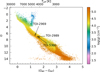 |
Fig. 1 HR diagram of all Gaia DR3 nearby stars with parallax π ≥ 10 mas, where the colors indicate log(g). The three stars presented in this work are overplotted and visible on the main sequence. |
3 Observations
The photometric data for the targets were acquired from the TESS mission (Section 3.1). Data from SOAR and SAI were employed in speckle interferometry to search for potential stellar companions (Section 3.2). Subsequent follow-up photometric observations involved El Sauce, PEST, LCO-CTIO, LCO-SAAO, LCO-HAL, TRAPPIST-South, Brierfield, and SUTO (Section 3.3). Ground-based high-resolution spectroscopic data were obtained using the CORALIE spectrograph (Section 3.4).
3.1 TESS photometry
Table 1 shows the sectors in which the three systems presented in this paper were observed by TESS, including the years and exposure times. For the analyses of these systems, we used the Presearch Data Conditioned Simple Aperture Photometry (PDC-SAP; Stumpe et al. 2012, 2014; Smith et al. 2012) fluxes and the corresponding errors, which were produced by the Science Processing Operation Center (SPOC; Jenkins et al. 2016). If no TESS -SPOC data was available, we instead used the Quick Look Pipeline (QLP; Huang et al. 2020b,a) photometry. Any data flagged for quality issues (e.g., scattered light, poor calibration, or insufficient targets for systematic error correction), recognizable by a quality parameter larger than 0, were excluded. Cosmic rays were mitigated on the satellite before downlink. The TESS data were accessed via the lightkurve Python package (Lightkurve Collaboration 2018).
For TOI-2969, the TESS sector 10 data are impacted by instrumental noise, as reflected in the notably higher σοοT relative to the other sectors. The two affected intervals of the light curve were excluded from the analysis. For TOI-5300, the TESS sector 70 light curve exhibits significantly more red noise than sector 42, with an out-of-transit jitter of 4720 ppm. These fluctuations occur on timescales comparable to the transit duration, compromising the transit signal’s reliability. Consequently, sector 70 was excluded from the analysis to ensure data quality and robustness.
Properties of the TESS -SPOC and QLP light curves.
3.1.1 TOI-2969 - TIC 36452991
TOI-2969 was alerted on 2021 June 04 (Guerrero et al. 2021) by the TESS Science Office (TSO) after detection by the FAINT transit search pipeline (Kunimoto et al. 2022) using QLP fullframe image (FFI) data from sectors 9, 10, and 36. The SPOC transit search pipeline (Jenkins 2002; Jenkins et al. 2010, 2020) also detected the signature in 2-min cadence data from sector 63. A difference image centroiding analysis located the host star within 0.95 ± 2.5″ of the transit source (Twicken et al. 2018).
3.1.2 TOI-2989 - TIC 97825640
TOI-2989 was detected by the FAINT pipeline using the QLP FFI light curve from sector 9. After vetting, the TSO issued a TOI alert on 2021 June 04. The SPOC transit planet search pipeline also detected the transit signal in sector 36 FFI light curve (Caldwell et al. 2020), with difference image centroiding locating the host star within 1.2 ± 2.5″ of the transit source.
3.1.3 TOI-5300 - TIC 267215820
TOI-5300 was detected by the FAINT pipeline using the QLP FFI light curve from sector 42. The TSO reviewed the vetting information and issued a TOI alert on 2022 Feb 28. The SPOC transit planet search pipeline also identified the transit signal in sectors 42 (FFI, 200-sec cadence) and 70 (2-min cadence). A difference image centroiding analysis placed the host star within 0.683 ± 2.5″ of the transit source.
3.2 Speckle Interferometry
3.2.1 SOAR
All stars in this paper were observed with the High-Resolution Camera (HRCAM) installed at the 4.1 m Southern Astrophysical Research (SOAR) telescope, located at Cerro Pachón, Coquimbo, Chile. Tokovinin (2018) describes the method for identifying stellar companions. In summary, the presence of binaries is determined from spatial Fourier transform images obtained through speckle observations. A companion star appears as fringes in these images. The autocorrelation function images, as shown in Figure A.1, are reconstructed images that include a companion to TOI-2969 (with a separation of 3.3″, Gaia DR3 5407977460534995840), and a mirrored counterpart resulting from the imaging process. The influence of this companion on the RV and photometric data is discussed in combination with the orbital solution in Section 5.1. The true position of the binary is determined using shift-and-added lucky imaging, which has a lower contrast sensitivity compared to speckle imaging. For TOI-2989 and TOI-5300, no stellar companions were detected, with detection limits of ΔI = 5.5m and ΔI = 6.0m, respectively, at 1.0″.
3.2.2 SAI
TOI-5300 was observed on UTC 2023 September 30 with the speckle polarimeter on the 2.5-m telescope at the Caucasian Observatory of the Sternberg Astronomical Institute (SAI) of Lomonosov Moscow State University. The image is visible in Figure A.2. A low-noise complementary metal oxide semiconductor (CMOS) detector, Hamamatsu ORCA-quest (Safonov et al. 2017), was used as a detector. The atmospheric dispersion compensator was active, which allowed use of the Ic band. The respective angular resolution was 0.083″. A total of 2500 frames with 60 ms exposure were accumulated. The atmospheric conditions were exceptionally good at the time of observation; the long-exposure full width at half maximum (FWHM) was 0.54″. We did not detect any stellar companions; detection limits are ΔIc = 4.7m and 6.2m at distances of 0.25″ and 1.0″ from the star, respectively.
3.3 Ground-based photometry
The TESS pixel scale is ~21″ pixel−1 and the photometric apertures typically extend to approximately 1′, generally causing multiple stars to blend into the TESS photometric aperture. The SPOC uses difference image centroiding to localize the transit source to typically 2.5″ (~0.1 pixels). To verify the true source of the TESS detection and to check for wavelength-dependent transit depth, we acquired ground-based time-series follow-up photometry of the fields around TOI-2969, TOI-2989, and TOI-5300 as part of TFOP. We used the TESS Transit Finder, which is a customized version of the Tapir software package (Jensen 2013), to schedule our transit observations. All light curve data are available on each host star’s web page on the Exoplanet Follow-up Observing Program (ExoFOP) website6 and are included in the global modeling described in Section 5.
3.3.1 TOI-2969
We observed a full transit window of TOI-2969 b on UTC 2021 June 12 in the Cousins R band from the Perth Exoplanet Survey Telescope (PEST) located near Perth, Australia. The 0.3 m PeSt telescope has a 5544 × 3694 QHY183M camera. Images were binned 2 × 2 in software, giving an image scale of 0.7″ pixel−1 and resulting in a 32′ × 21′ field of view. A custom pipeline based on C-Munipack7 was used to calibrate the images and extract the differential photometry. We used circular photometric apertures of 7.1″ that included all of the flux from the nearest known neighbor in the Gaia DR3 catalog (Gaia DR3 5407977460534995840), which is 3.4″ northeast of TOI-2969 and three magnitudes fainter in the TESS band.
Two full transit windows were observed on 2021 December 19 and 2022 March 05 in the i′ and g′ bands, respectively, from the Las Cumbres Observatory Global Telescope (LCOGT) 0.4m network nodes at Cerro Tololo Inter-American Observatory (CTIO), and the South African Astronomical Observatory near Sutherland, South Africa (SAAO). We used circular photometric apertures of 3.9″ and 3.5″, respectively, that were ~50% contaminated by the 3.4″ companion.
We observed a full transit window on UTC 2022 March 02 in the Johnson-Cousins R band using the Evans 0.36m telescope at El Sauce Observatory. We used a circular photometric aperture of 4.3″ that included part of the flux from the 3.4″ neighbor. We also used a circular photometric aperture of 1.6″ that excluded most of the flux from the 3.4″ neighbor, showing that the event occurs in TOI-2969. We used the larger aperture light curve in the global modeling since blending from the neighbor was only ~3%, and because the smaller aperture light curve has much larger noise.
One full transit window was observed on 2022 November 24 in the B band using the Silesian University of Technology (SUTO) 0.3 m telescope located in Pyskowice, Poland. The SUTO telescope is equipped with a 4656 × 3520 pixel Atik 11000M camera with an image scale of 0.712″ pixel−1, resulting in a 38′ × 26′ field of view. The differential photometric data were extracted using AstroImageJ, using circular photometric apertures of 3.9″.
We observed two more full transit windows on UTC 2023 February 25 and 2023 March 28 in the z′ and B bands using the TRAnsiting Planets and PlanetesImals Small Telescope (TRAPPIST) South 0.6m telescope located at La Silla Observatory (Chile) (Jehin et al. 2011; Gillon et al. 2011). TRAPPIST-South is equipped with an FLI camera with an image scale of 0.6″ pixel−1, resulting in a 22′ × 22′ field of view. The image data were calibrated, and photometric data were extracted using a dedicated pipeline that uses the prose framework described in Garcia et al. (2022). We used circular photometric apertures of 3.5″ and 5.0″ that included the flux from the 3.4″ neighbor. An approximately on-time ~23 ppt event was detected in all seven observations.
3.3.2 TOI-2989
We observed a full transit window of TOI-2989 b on UTC 2024 January 16 in the Johnson/Cousins R band from the Evans 0.36 m telescope at El Sauce Observatory. We used circular photometric apertures of 5.4″ that excluded all of the flux from the nearest known neighbor in the Gaia DR3 catalog (Gaia DR3 3531594171179942528), which is ~37″ southeast of TOI-2989. An approximately on-time ~28 ppt event was detected on target.
A partial and a full transit window were also observed with TRAPPIST-South on UTC 2022 April 25 and 2022 May 17 in the NIR 700 nm long-pass band and B band, using circular photometric apertures of 5.1″ and 3.8″, respectively. An approximately on-time ~28 ppt event was detected on target in both observations.
Characteristics of the CORALIE observations.
3.3.3 TOI-5300
We observed a full transit window on UTC 2022 June 22 in the Cousins R band using the Brierfield Observatory near Bowral, New South Wales, Australia. The 0.36 m telescope is equipped with a 4096 × 4096 Moravian 16803 camera. The image scale after binning 2 × 2 was 1.47″ pixel−1, resulting in a 50′ × 50′ field of view. The differential photometric data were extracted using AstroImageJ with a circular 8.8″ photometric aperture that excluded all of the flux from the nearest known neighbor in the Gaia DR3 catalog (Gaia DR3 2642761924907362560), which is ~52″ south of TOI-5300.
Two full transit windows were observed on UTC 2022 July 08 and 2020 October 18 in the Sloan i and g bands, respectively, from the LCOGT 0.4m network node at Haleakala Observatory on Maui, Hawai’i (HAL). The photometric data were extracted using circular apertures of 6.6″ for Sloan i and 8.8″ for Sloan g. Another full transit window was observed on UTC 2022 August 09 in the Sloan g band using the LCOGT 0.4m network node at CTIO. The photometric data were extracted using circular 8.8″ photometric apertures.
We observed one full transit window on UTC 2022 August 26 in the Johnson-Cousins V band using TRAPPIST-South. The photometric data were extracted using circular 3.8″ photometric apertures. An ~23 ppt event was detected on target in all observations.
3.4 CORALIE spectroscopy
Spectroscopic vetting and RV observations were performed with the CORALIE echelle spectrograph at the Swiss 1.2m Leonhard Euler telescope at La Silla Observatory (Chile) (Queloz et al. 2001). All observations were conducted out of transit, ensuring that the Rossiter-McLaughlin effect did not affect the data. The CORALIE data were accessed using dace-query, a Python package from the Data & Analysis Center for Exoplanets8. The RVs were derived by version 3.8 of the CORALIE Data Reduction System (DRS), which employs the CCF with numerical stellar templates closely matched to the spectral types of each TOI (in this case, K5). The DRS provides the RVs, the FWHM, the bisector span, and the contrast. Additionally, the pipeline provides data on the activity indices derived from the Na, Ca, and Hα lines. Table 2 provides an overview of the CORALIE data we obtained for our analysis.
To exclude potential diluted binaries, the data were also reduced using other stellar masks with spectral types further from our stars (A0, F0, G5, and M2). In binary systems with components of different spectral types, applying different stellar masks can enhance the contribution of the companion to the CCF, potentially shifting the measured RV, as demonstrated in the case of HD 41004 (Santos et al. 2002). Our analysis did not reveal any significant mask effects. Furthermore, all RV observations were checked for strong correlations with stellar activity indicators. However, short-period stellar activity, such as starspots or flares, typically causes small RV variations (root mean square (RMS) ~2-10 m/s Cretignier et al. 2020). The significant RV variations (RMS ranging from 100 to 400 m/s) observed in our three stars suggest an external influence, likely from a companion, rather than intrinsic stellar activity.
Stellar parameters of the stars presented in this paper.
4 Stellar properties
Table 3 provides an overview of the stellar properties. The spectral type was derived from the effective temperature, using Table 5 of Pecaut & Mamajek (2013). The magnitudes H, K, V, and B originate from the TESS Input Catalog (TIC) working group (Paegert et al. 2021; Stassun et al. 2019), as the stars are too faint to have been observed by Tycho (ESA 1997). The log R′HK values are not reported, as the flux in the H and K bands are insufficient in the CORALIE data. The right ascension α, declination δ, proper motions in both directions (μα★,μδ), parallax π, and the derived distance d originate from Gaia DR3 (Gaia Collaboration 2023). The effective temperature Teff, the microturbulence vtur, and the metallicity [Fe/H] are results of the spectral analysis, described in more detail in Section 4.1. The extinction AV, the bolometric luminosity Lbol, the stellar radius R★, and the stellar mass M★ are derived from the spectral energy distribution (SED) analysis, described in Section 4.3. The surface gravity, log(g), is computed using the stellar density derived in Section 5 and the stellar radius.
The reported FWHM represents the average of the FWHM values derived from the CCF, obtained by correlating the CORALIE stellar spectra with a K5 mask. The standard deviation of these values was used as the error. A higher standard deviation in the FWHM may indicate greater stellar activity, as it reflects variations in spectral line widths. The rotational velocity v sin i is an approximation based on the FWHM adapted from Santos et al. (2002). The rotational period was approximated from the public Gaia DR3 photometric data (Section 4.4.1), and/or the WASP transit survey (Section 4.4.2).
4.1 Spectral analysis
The stellar spectroscopic parameters (Teff, vtur, [Fe/H]) were derived using the ARES+MOOG methodology, which is described in detail in Sousa et al. (2021); Sousa (2014); Santos et al. (2013). To consistently measure the equivalent widths (EWs), we used the ARES code9 (Sousa et al. 2007, 2015). The spectral analysis was performed using the combined spectrum obtained by shifting to the measured RV and taking the mean of the individual exposures for each star. In this analysis, we used the list of lines presented in Tsantaki et al. (2013), which is suitable for stars with Teff < 5200 K. The best set of spectroscopic parameters for each spectrum was found using a minimization process to achieve ionization and excitation equilibrium. This process uses a grid of Kurucz model atmospheres (Kurucz 1993) and the latest version of the MOOG radiative transfer code (Sneden 1973).
The effective temperatures from different sources.
4.2 Effective temperatures
Given the significant discrepancy (200-400 K) between the effective temperatures obtained from our spectral analysis and those in the TESS Input Catalog (TICv8; Stassun et al. 2019), caution is advised when relying on TICv8 values for effective temperature estimates. Our analysis indicates that all the stars in our sample exceed the selection criterion of Teff < 4600 K and are generally more consistent with effective temperatures from the General Stellar Parametrizer from Photometry (GSP-Phot) library of Gaia DR3, except for TOI-2969 (see Table 4). We adopted the spectroscopic values, which are directly derived from our observations, to ensure consistency.
4.3 SED analysis
As an independent determination of the basic stellar parameters, we performed an analysis of the broadband SEDs of the stars together with the Gaia DR3 parallaxes (with no systematic offset applied; see, e.g., Stassun & Torres 2021). This analysis was conducted to determine an empirical measurement of the stellar radii, following the procedures described in Stassun & Torres (2016); Stassun et al. (2017, 2018). We obtained the JHKS magnitudes from 2MASS, the W1-W3 magnitudes from WISE, and the GBP and GRP magnitudes, as well as the absolute flux-calibrated spectrophotometry, from Gaia. Together, the available photometry spans the full stellar SED over the wavelength range 0.4-10 μm (see Figure B.1).
We performed a fit using PHOENIX stellar atmosphere models (Husser et al. 2013), with Teff, log g, and [Fe/H] set to the previously determined values. The extinction AV was limited to the maximum line-of-sight value from the Galactic dust maps of Schlegel et al. (1998). Integrating the (unreddened) model SED gives the bolometric flux at Earth, Fbol. Using Fbol and the Gaia parallax, we then derived the bolometric luminosity, Lbol. The Stefan-Boltzmann relation was then used to derive the stellar radius, R★. Finally, we estimated the stellar mass, M★, from appropriate empirical relations depending on the stellar mass (i.e., Torres et al. 2010).
4.4 Rotational period
4.4.1 Gaia
TOI-2969 and TOI-2989 are flagged as variable in Gaia DR3. Variability in stars can arise from multiple origins. The classification used in the variability processing (Eyer et al. 2023) can be found in the variability summary database gaiadr3.vari_summary. For both stars, the variability flag arises from solar-like variability, which can originate from flares, stellar spots, and/or chromospheric variability. When Gaia flags a star as variable, the corresponding epoch photometry becomes publicly available. Thus, we were able to access the Gaia photometric data for these two stars.
Performing a Lomb-Scargle periodogram on the photometric data (combining the three available magnitudes G, GBP, and GRP), we identified potential rotational periods (see Appendix C). TOI-2969 has a potential rotational period of 26.8 ± 2.0 days, visible in GBP and GRP . In the G band, a period of 16 ± 10 days is visible, and a similar period of 19 ± 10 days also appears in all three magnitudes when using a window function. Since both potential rotational periods fall within the range identified by the window function, the rotational period remains uncertain, but the 26.8-day signal is more probable. TOI-2989 has a rotational period of 29.2 ± 1.5 days visible in all three magnitudes. This is not due to data sampling, as it does not appear in the window function.
Gaia photometric errors are underestimated due to uncalibrated systemic errors (Evans et al. 2023). When adding 1% to the noise, the Lomb-Scargle periodogram still identifies the rotational periods as significant above 1% false alarm probability (FAP). These rotational periods are not detected in the TESS data (from which the short-period companion transits are excluded) when using a box-fitting least squares (BLS) algorithm (Kovács et al. 2002), nor when computing the Lomb-Scargle periodogram. This is due to the absence of consecutive TESS sectors, which limits the data to a 27-day span. While BLS is not expected to detect stellar rotation periods from spot-modulated light curves due to its focus on identifying low-duty-cycle transitlike features, the absence of a signal in the BLS search suggests that the modulation is unlikely to be caused by a transit. This is more challenging to confirm with the lower cadence Gaia data.
After removing the rotational period variation, the transit periods do not appear when a BLS is performed on the resulting Gaia data. When phase-folding the Gaia photometric data to the period and epoch from the orbital solution presented in Section 5, TOI-2969 and TOI-2989 show a change in flux at the time of transit. This shows that, in principle, Gaia has detected the transit. Although the data exhibit significant scatter (see Figure 2).
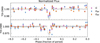 |
Fig. 2 Phase-folded Gaia photometric data. Colored points indicate the different Gaia wave bands. The black points show the TESS data, binned in intervals of 1/1000 of the period. The errors in the Gaia data are corrected following Evans et al. (2023) by adding an error in quadrature as a function of the magnitude. Long-period signals above 0.01% false alarm probability (FAP) are subtracted, and the errors are scaled by the ratio of the standard deviation before and after signal subtraction. |
4.4.2 WASP
We obtained data from the WASP transit survey (Pollacco et al. 2006) to search for rotational modulations of the host stars. WASP data were collected using Canon 200-mm, f/1.8 lenses backed by 2048 × 2048 CCDs, observing with a 400-700 nm passband, and producing photometry from extraction apertures with a radius of 48″ centered on each star (Pollacco et al. 2006). We searched the accumulated light curves for periodicities in the range of 1 to 130 days using methods discussed in Maxted et al. (2011) (see Appendix D for the WASP light curve periodograms).
For TOI-2969, WASP-South recorded 12 840 data points between 2006 and 2012. No significant rotational modulation was detected, given that the amplitude of the Gaia modulation is three times lower for TOI-2969 (~5 mmag) than for TOI-2989 (~15 mmag), WASP likely does not have the sensitivity to detect the rotation seen by Gaia. In addition, the WASP extraction aperture contains multiple stars of similar brightness. Therefore, any detected modulation could not be attributed to a specific star. However, while TOI-2969 b was never a WASP candidate, knowing the TESS ephemeris, we find that the standard WASP transit-search algorithm (Collier Cameron et al. 2007) detects a tentative transit, giving an ephemeris of
![Mathematical equation: {\rm Transit [TDB(JD)]} = 245\,5830.9392 \pm\ 0.0035 \\ + N \times 1.823808 \pm\ 0.000052.](/articles/aa/full_html/2025/08/aa53879-25/aa53879-25-eq1.png)
This likely represents the first recorded data for the TOI-2969 b transit. However, given that the WASP precision is insufficient to improve the ephemeris and may introduce noise without significantly enhancing the results, the data were not included in the joint fit.
TOI-2989 was observed by WASP-South over the span of approximately 165 nights in 2009 and 2010, obtaining 15 000 data points. The 2010 data show a significant modulation in a period of 15.0 ± 0.5 d with an amplitude of 5 mmag and a false alarm likelihood below 2%. The 2009 data show a significant periodicity compatible with twice this period (30 ± 3 d), and an amplitude of 7 mmag. To check whether this might be caused by moonlight, we performed a similar analysis of several nearby stars in the field of view, but did not find the modulation. We are likely detecting a rotational modulation of TOI-2989 at a period of 30 ± 1 d, with its first harmonic present in the data from 2010. This is consistent with the rotational period observed in the Gaia variability data.
TOI-5300 was observed by WASP-South over the span of approximately 140 nights in 2008 and 2009, producing 9500 data points. The 2009 data show a significant modulation at a period of 15.6 ± 0.6 d, with an amplitude of 6 mmag and a false alarm likelihood below 1%. The 2009 data show a marginal detection (10% false alarm likelihood) of a modulation compatible with twice this period (32 ± 3 d). We also checked for moonlight interference by performing a similar analysis of nearby field stars, but these do not show the modulation. We are likely detecting a rotational modulation at a period of 31.2 ± 1.2 d, with its first harmonic present in the data from 2010. Given the 6 mmag amplitude, the signal should be visible in the Gaia G-band photometry, which has a median uncertainty of 0.2 mmag for a G magnitude of approximately 13 (Riello et al. 2021).
5 Orbital solutions
To derive the orbital solution, a joint-fit analysis, combining RV and photometric data, was performed using the Python software Juliet (Espinoza et al. 2019). The Dynamic Nested Sampling package dynesty (Speagle 2020) was used as a sampler to estimate Bayesian posteriors and evidence. Given that the RV variations aligned well with the photometric data, no Gaussian Process (GP) model was added to account for stellar activity. For CORALIE, accidental off-target observations were excluded from the analysis (e.g., no star in the fiber, verifiable via the integrated guiding frame images).
Table E.1 presents the priors used for the joint modeling. The estimated values for the orbital period P, time of transit T0, and stellar density ρ★, were obtained from the ExoFOP website6. The TESS limb darkening q1 and q2 parameters were calculated using the quadratic law, as described by Kipping (2013a), via LDCU10, a modified version of the Python code limb-darkening (Espinoza & Jordán 2015). The eccentricity e and the argument of periastron ω were treated in two ways: either both were fixed (e = 0 and ω = 90°), or e followed a beta prior with parameters as defined by Kipping (2013b), while ω was assigned a uniform prior ranging from 0 to 180 degrees. The log-evidence was used to compare the models and determine whether having e and ω free or fixed provided the best fit of the data. The radius ratio Rpl/R★ and the impact parameter b were assigned a uniform prior ranging from 0 to 1. Based on the absence of V-shaped transit features, the transits are not grazing; thus, b values larger than 1 were not considered. All other priors used values as suggested by the Juliet documentation. The resulting posterior distributions are presented in the form of corner plots in Appendix G (Foreman-Mackey 2016).
To evaluate the presence of contaminating sources with a threshold of six magnitudes difference, we utilized tpfplotter to display the average image of the target pixel files generated by TESS-SPOC (Aller et al. 2020). The sectors in which our three TOIs were observed and assessed for contamination are outlined in Table 1. For TOI-2989 and TOI-5300, across all sectors, the apertures used by TESS for light curve extraction are uncontaminated by neighboring stars. However, TOI-2969 is affected by contamination; we expect a maximum of approximately 3035% contamination from nearby stars. A dilution factor was included as a uniform prior from 0 to 1 for the ground-based photometry and the QLP light curves of TOI-2969. The QLP and TESS-SPOC data were treated as separate instruments with their own instrumental parameters in the joint fit, except for limbdarkening, which was shared due to the identical wavelength range, and therefore must have the same value. Since the PDC-SAP light curves account for contamination, a dilution factor was not included for TESS-SPOC data. All ground-based follow-up photometry was detrended for airmass using a linear regression model.
Table 5 presents the orbital solutions derived using Juliet. The fitted and instrumental parameters are taken from the model, with errors corresponding to the 1σ Monte Carlo uncertainties, while the derived parameters were subsequently computed. Specifically, the planetary radius Rpl is obtained from the stellar radius and the radius ratio; the planetary mass Mpl is determined using the RV equation (for transiting planets, Mpl sin i ≈ Mpl, assuming i ≈ 90°); and the bulk planetary density ρpl is calculated from Rpl and Mpl. The semi-major axis apl is derived from Kepler’s third law. The inclination i and the transit duration T14 are computed following the method detailed in Seager & Mallen-Ornelas (2003) and Kipping (2014), respectively. The planet equilibrium temperature Teq is determined from Teff, R★, and apl, assuming a Bond albedo A = 0. The insolation flux Spl is calculated from L and apl. The limb darkening coefficients and the photometric instrumental parameters are listed in the appendix F.
Fitted and derived parameters for the companions presented in this paper.
5.1 TOI-2969 b
TOI-2969 b is a hot Jupiter orbiting its K3V host with an orbital period of just 1.82 days. At its proximity of 0.0261 AU, the equilibrium temperature is 1186 K and receives an insolation of 382 S⊕. The planet is more massive than Jupiter, with a mass of 1.16 MJup and a radius of 1.10 RJup.
TOI-2969 has a stellar companion separated by 3.34″, as observed by HRCam with SOAR (Tokovinin 2018). Gaia DR3 (Gaia Collaboration 2023) also shows two sources within 3.4″ (Gaia DR3 5407977460534995840 and Gaia DR3 5407977460540294784, the latter being TOI-2969); however, their parallaxes differ significantly (0.106 mas and 6.153 mas, respectively), indicating that these stars do not belong to the same system. Contamination of the RV signal from the nearby star is negligible, as it is 3.1 mag fainter in G magnitude, located outside the 2″ CORALIE fiber, and resolved, given that we do not observe under seeing conditions worse than 1.8″. All fitted photometry contamination values are smaller than our maximally expected 30-35% (see Fig. 6). Relative to the groundbased photometry, QLP has the highest contamination (21%), which is expected as TESS uses the largest photometric window. As the transit is confirmed on target (see Section 3.3.1), the RV variation seen for TOI-2969 can be attributed to a giant companion with a planetary mass of 1.16 MJup. The Juliet fit does not include the eccentricity or the argument of periastron, as they do not improve the model. The resulting model compared to the RV and photometric data is shown in Figures 3 and 6. No significant signs of additional planets were detected; the CORALIE jitter is consistent with zero.
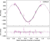 |
Fig. 3 Overlay of TOI-2969’s orbital solution with CORALIE RV observations, with residuals shown in the lower panel (RMS of 23 m/s). |
5.2 TOI-2989 b
TOI-2989 is a high proper motion star, which may indicate a different evolutionary pathway or membership in a Residuals with an RMS of 112 m/s are shown in the lower panel.
Galactic kinematic population. A quick approximation combining proper motion and parallax shows that its tangential velocity is ~ 110 km/s. When combined with the systemic velocity measured by CORALIE, the total velocity is also around 110 km/s. This would potentially place the star in the thick disk population (Nissen 2004). It hosts a hot Jupiter with an orbital period of 3.12 days and is located at apl = 0.0384 AU, resulting in Teq = 1001 K and receiving insolation 124 times that of Earth. The planet’s radius of 1.12 RJup and a mass of 3.0 MJup suggest that it has a massive gaseous envelope.
The Juliet fit did not improve with the addition of the eccentricity and the argument of periastron, and thus these parameters were not included. The resulting models, along with the RV residual with an RMS value of 112 m/s, are shown in Figure 4, and the photometric observations in Figure 7. A fluctuation is visible at the ingress in the El Sauce data. The TESS light curves were checked for similar depth fluctuations, and the BLS analysis of sector 9 identified an 11.8-day period, caused by a dip at the edge of the sector. No corresponding signal was found in sector 36. Given that the El Sauce data are ground-based and no matching signal appears in the TESS light curves, the fluctuation is most likely due to instrumental systematics or external factors such as weather variability. The data show no clear indications of further planets; the CORALIE jitter is consistent with zero.
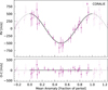 |
Fig. 4 Orbital solution for TOI-2989 alongside its CORALIE RV data. |
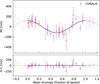 |
Fig. 5 Orbital solution for TOI-5300 superimposed on CORALIE RV data, with residuals plotted in the lower panel (RMS of 68 m/s). |
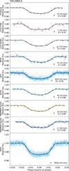 |
Fig. 6 Phase-folded TESS light curve of TOI-2969. The Juliet fit is shown as a black line, while TESS data is plotted in light blue in the lower panel. The upper panels feature ground-based follow-up photometric observations from LCO-SAAO, LCO-CTIO, TRAPPIST-South, El Sauce, SUTO, and PEST. Data points with black-edged markers indicate 10-minute bins, except for LCO-SAAO (g′) observations, which are binned by 15 minutes. If the dilution D is fitted, it is indicated per light curve, otherwise, it is set to 1. |
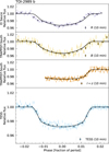 |
Fig. 7 Phase-folded TESS light curve of TOI-2989. The Juliet fit is shown as a black line, while TESS data is plotted in light blue in the lower panel. The upper panels feature ground-based follow-up photometric observations from El Sauce and TRAPPIST-South. Data points with black-edged markers indicate 10-minute bins. |
5.3 TOI-5300 b
TOI-5300 b orbits its K4V host in 2.26 days. The planet’s radius, Rpl = 0.88RJup, and mass, Mpl = 0.6MJup, are smaller than those of Jupiter, giving it a bulk density of 1.1 g cm−3. At its proximity of 0.0236 AU, it receives an insolation of 198 S⊕, resulting in Teq = 1043 K. The hot Jupiter TOI-5300 appears to be the only planet in its system, as no robust evidence supports additional planets, and the CORALIE jitter is consistent with zero. Figures 5 and 8 show the resulting orbital solution. As with the other hot Jupiters presented in this paper, the Juliet fit did not improve when including eccentricity and the argument of periastron as free parameters, so these were fixed at e = 0 and ω = 90°.
6 Discussion
We confirm the presence of three hot Jupiters orbiting mid-K dwarfs: TOI-2969 b, TOI-2989 b, and TOI-5300 b. Figure 9 shows these companions compared to known transiting exoplanets, highlighting their location in a relatively poorly populated region of the diagram. Characterizing these objects contributes to filling the low-mass star ends of the exoplanet distribution, enriching our understanding of planetary demographics.
6.1 Heavy element masses
The heavy element content of the three hot Jupiters, TOI-2969 b, TOI-2989 b, and TOI-5300 b, is estimated using interior models.
According to the empirical formulas of Sestovic et al. (2018), TOI-2969 b, TOI-2989 b, and TOI-5300 b should not be inflated, as the insolation does not exceed the threshold in incident flux. Indeed, when applying the Fortney et al. (2007) models that do not include inflation, TOI-2969 b can be explained by a 50 M⊕ core mass at an approximate age of 4.5 Gyr. Similarly, TOI-2989 b is consistent with a 100M⊕ core mass at 1 Gyr, and TOI-5300 b with a 100M⊕ core mass at 4.5 Gyr.
However, the three planets can also be described by models that include inflation. Applying the models from Baraffe et al. (2008) with typical hot Jupiter irradiation (equivalent to solar exposure at 0.045 AU) and using approximate values for age and heavy element fraction (derived from the fitted interior models presented later in this section), we find the following theoretical radii: For TOI-2969 b, assuming an age of around 3 Gyr and a heavy element mass fraction of Z = 0.10, the radius is predicted to be close to 1.06RJup. For TOI-2989 b, with an assumed age of about 1 Gyr and the same heavy element fraction, the radius is predicted to be near 1.09RJup. For TOI-5300 b, assuming an age of approximately 3 Gyr and a higher metallicity of Z = 0.50, the expected radius is approximately 0.77RJup. These estimated radii correspond well with the observed values, which are 1.10 ± 0.08RJup, 1.12 ± 0.05RJup, and 0.83 ± 0.07RJup, respectively. To test whether these planets can also be fitted when including heating efficiency leading to radius inflation, we use the grid of interior models for hot Jupiters published by Sarkis et al. (2021). These models, based on the planetary evolution code completo (Mordasini et al. 2012b), assume a composition of an H/He envelope, without a central core (using the SCvH equation of state (EoS); Saumon et al. 1995), in which heavy elements are modeled as water (ANEOS equation of state Thompson 1990) and are assumed to be homogeneously mixed. The envelope is coupled with a fully non-gray atmospheric model from petitCODE (Mollière et al. 2015, 2017). This grid of interior models does not trace the planet’s evolution over time, but relies on the internal luminosity value to estimate the planetary internal structure. We adopt a uniform prior on the internal luminosity; as noted in Sarkis et al. (2021), the choice of the prior impacts the derived luminosity and the heating efficiency coefficient. However, we find that the heavy element fractions are compatible at 1 σ when a log-uniform prior is used. The fraction of heavy elements in the interior is 0.24 ± 0.08, 0.12 ± 0.03, and 0.44 ± 0.08 for TOI-2969 b, TOI-2989 b, and TOI-5300 b, respectively. From the fraction of heavy elements, the heavy-element mass can be derived (e.g., Ulmer-Moll et al. 2022), and we find that TOI-2969 b, TOI-2989 b, and TOI-5300 b contain significant heavy element masses of 88 ± 30M⊕, 114 ± 30M⊕, and 84 ± 21M⊕, respectively. Compared with other studies discussing the heavy-element mass of companions orbiting K dwarfs (e.g. Hartman et al. 2009, 2011; Grunblatt et al. 2017; Torres et al. 2008; Hacker et al. 2024; Delamer et al. 2024; Hellier et al. 2010), our three targets have relatively high heavy-element masses, which is linked to their higher densities.
The inclusion of heating efficiency does not significantly impact the radii of TOI-2989 b and TOI-5300 b. For these two planets, the inferred heavy element content is consistent between models with and without inflation. However, for TOI-2969 b, including inflation impacts the planetary radius, resulting in a larger estimated heavy element content when modeled with inflation. TOI-2969 b may be more affected by additional heating efficiency, as it has the lowest density in the sample and receives the highest stellar irradiation, leading to an equilibrium temperature of 1186 K. This highlights the degeneracy between incorporating additional heating efficiency, which increases the planetary radius, and adding heavy elements to the interior, which decreases the overall radius.
In conclusion, all planets can be modeled without including additional heating efficiency and are found to contain a significant amount of heavy elements. We note that the models used in this work rely on the SCvH equation of state for H/He and that more recent EoS from Chabrier & Debras (2021) typically result in smaller planetary radii and a lower amount of heavy elements (e.g. Müller et al. 2020).
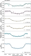 |
Fig. 8 Phase-folded TESS light curve for TOI-5300. The Juliet model fit is depicted as a black line, while TESS data shown in light blue in the lower panel. The upper panels include ground-based photometric observations from LCO-CTIO, LCO-HAL, TRAPPIST-South, and Brierfield. Data points with black-edged markets indicate 10-minute bins for TESS, Brierfield, and TRAPPIST-South, 15-minute intervals for LCO-CTIO and LCO-HAL (i′), and 30-minute intervals for LCO-HAL(g′). |
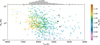 |
Fig. 9 Overview of the presented companions (encircled in red) compared to known planets from the PlanetS catalog (extended from Otegi et al. (2020); Parc et al. (2024), updated August 2024). The data are color coded by planetary radii. The histogram at the top shows the relative occurrence of the transiting gas giants with masses ranging from 0.1 to 13 MJup. The low-mass star regime remains relatively poorly populated; our three mass characterizations contribute to this population. |
6.2 Planet-metallicity correlation
Metal-rich stars are more likely to host giant exoplanets, consistent with the planet-metallicity correlation for FGK stars (Ida & Lin 2004; Santos et al. 2004; Fischer & Valenti 2005). This correlation appears particularly true for low-mass stars, where the expected lower disk mass of M dwarfs (Vorobyov & Basu 2008; Alibert et al. 2011) can be compensated for by a higher metallicity (and vice versa) (Thommes et al. 2008; Mordasini et al. 2012a). Our stars, with masses between 0.67 and 0.77 M, exhibit [Fe/H] metallicities of 0.08 ± 0.05, −0.04 ± 0.07, and −0.17 ± 0.07, which align with, or slightly exceed, the average metallicity expected for K dwarfs of similar mass (e.g. Fig. 9 from Fischer & Valenti 2005), where [M/H] ≈-0.15 is typical. Since [M/H] represents the total metal abundance and is greater than or equal to [Fe/H], these values can be directly compared. Guillot et al. (2006); Fortney et al. (2006) have shown that the metal content of a planet correlates with that of its host star. Given the significant uncertainty in metallicity and heavy element masses, determining whether these three targets agree with the correlation is complex.
6.3 Eccentricity
All orbital solutions presented in this paper fix the eccentricity and the argument of periastron at constant values (e = 0 and ω = 90°). When allowing these parameters to vary, we determine 3 σ upper limits on the eccentricity of 0.01 for TOI-2969 b, 0.03 for TOI-2989 b, and 0.05 for TOI-5300 b. The argument of periastron does not converge. We find that TOI-2969 b, TOI-2989 b, and TOI-5300 b are best described by models with fixed circular orbits (e = 0) based on the Juliet fits’ log-evidence values. This is consistent with the expectation that most hot Jupiters, especially those with orbital periods up to approximately three days, have circularized orbits. If these planets initially had elliptical orbits, they would have quickly circularized due to the strong tidal dissipation caused by their proximity to their host stars (Hut 1981).
6.4 Multiplicity
Hot Jupiters typically lack nearby planetary companions, likely because their inward migration clears out planets in close orbits. The planetary systems of WASP-132 (Grieves et al. 2025) and TOI-1130 (Borsato et al. 2024) are notable exceptions among K dwarfs, each hosting an inner short-period super-Earth alongside a hot Jupiter. Within the precision of our CORALIE data, there are no indications of additional companions with periods up to ~1 year, as all jitter values are consistent with zero. Nonetheless, these targets remain relevant for additional RV follow-up observations, as 52 ± 5% of hot Jupiters have additional, longer period companions, as shown by Bryan et al. (2016).
6.5 Atmospheric characterization
With orbital periods shorter than four days, the three planets presented in this paper can also be considered for atmospheric characterization. The indicators most commonly used for the expected signal-to-noise ratio (S/N) of transmission and emission spectroscopy are the transmission spectroscopy metric (TSM) and the emission spectroscopy metric (ESM), as defined by Kempton et al. (2018). TOI-2969 has an elevated ESM of 149, a TSM of 90, and a relatively large scale height of 205 km, suggesting it is promising for atmospheric studies. In contrast, TOI-2989, with an ESM of 71, aTSMof20, and a scale height of 70 km, is less favorable for atmospheric studies. TOI-5300, with an ESM of 76, a TSM of 77, and a large scale height of 224 km, also shows potential for atmospheric characterization, though it is not as favorable as TOI-2969.
7 Conclusions
We confirm and characterize three non-inflated hot Jupiters -TOI-2969 b, TOI-2989 b, and TOI-5300 b - orbiting mid-K dwarfs. These mass measurements highlight the importance of spectroscopic follow-up, as they contribute to the growing, well-characterized catalog of gas giants around low-mass stars. These stars are part of an ongoing CORALIE program that should provide further characterizations in the future. The unique characteristics of the discovered objects, e.g., non-inflated hot Jupiters with a significant amount of heavy elements, offer valuable opportunities for future research in planetary and substellar science, such as atmospheric studies and low-mass star formation. TOI-2969 b stands out as the most promising target for emission spectroscopy.
Acknowledgements
The authors thank the ESO staff at La Silla for operating and maintaining the instruments for so many years. A special thanks to Laurent Eyer for his assistance in accessing and inspecting the Gaia photometric data. This work has been carried out within the framework of the NCCR PlanetS supported by the Swiss National Science Foundation under grants 51NF40_182901 and 51NF40_205606. Funding for the TESS mission is provided by NASA’s Science Mission Directorate. We acknowledge the use of public TESS data from pipelines at the TESS Science Office and the TESS Science Processing Operations Center. This research has made use of the Exoplanet Follow-up Observation program (ExoFOP; DOI: 10.26134/ExoFOP5) website, which is operated by the California Institute of Technology, under contract with the National Aeronautics and Space Administration under the Exoplanet Exploration program. Resources supporting this work were provided by the NASA High-End Computing (HEC) program through the NASA Advanced Supercomputing (NAS) Division at Ames Research Center for the production of the SPOC data products. This paper includes data collected by the TESS mission that are publicly available from the Mikulski Archive for Space Telescopes (MAST). The research leading to these results has received funding from the ARC grant for Concerted Research Actions, financed by the Wallonia-Brussels Federation. TRAPPIST is funded by the Belgian Fund for Scientific Research (Fond National de la Recherche Scientifique, FNRS) under the grant PDR T.0120.21. Based in part on observations obtained at the Southern Astrophysical Research (SOAR) telescope, which is a joint project of the Ministério da Ciência, Tecnologia e Inovações (MCTI/LNA) do Brasil, the US National Science Foundation’s NOIRLab, the University of North Carolina at Chapel Hill (UNC), and Michigan State University (MSU). KAC and CNW acknowledge support from the TESS mission via subaward s3449 from MIT. SGS acknowledges the support from FCT through Investigador FCT contract nr. CEECIND/00826/2018 and POPH/FSE (EC). NCS acknowledges funding by the European Union (ERC, FIERCE, 101052347). Views and opinions expressed are however those of the author(s) only and do not necessarily reflect those of the European Union or the European Research Council. Neither the European Union nor the granting authority can be held responsible for them. This work was supported by FCT - Fundação para a Ciência e a Tecnologia through national funds by these grants: UIDB/04434/2020, UIDP/04434/2020. IAS acknowledges the support of M.V. Lomonosov Moscow State University program of Development. This work makes use of observations from the LCOGT network. The postdoctoral fellowship of KB is funded by F.R.S.-FNRS grant T.0109.20 and by the Francqui Foundation. MG and EJ are F.R.S.-FNRS Research Directors. This publication benefits from the support of the French Community of Belgium in the context of the FRIA Doctoral Grant awarded to MT. We acknowledge financial support from the Agencia Estatal de Investigación of the Ministerio de Ciencia e Innovaciôn MCIN/AEI/10.13039/501100011033 and the ERDF “A way of making Europe” through project PID2021-125627OB-C32, and from the Centre of Excellence “Severo Ochoa” award to the Instituto de Astrofisica de Canarias. AP was financed by grants 02/140/RGJ24/0031 and BK 2025. FJP acknowledges financial support from the Severo Ochoa grant CEX2021-001131- S MICIU/AEI/10.13039/501100011033 and Ministerio de Ciencia e Innovación through the project PID2022-137241NB-C43. MS acknowledges financial support from the Swiss National Science Foundation (SNSF) for project 200021_200726.
Appendix A Speckle Interferometry Images
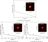 |
Fig. A.1 Speckle observations from SOAR. |
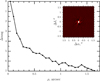 |
Fig. A.2 SAI speckle interferometry - TOI-5300, UTC 2023 September 30 |
Appendix B SED analysis
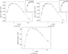 |
Fig. B.1 The spectral energy distributions (SEDs). Red symbols represent the observed photometric measurements, and the horizontal bars represent the effective width of the passband. Blue symbols are the model fluxes from the best-fit PHOENIX atmosphere model (black). The insets show the absolute flux-calibrated Gaia spectrophotometry as a gray swathe overlaid on the model (black). |
Appendix C Gaia DR3 Photometry
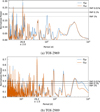 |
Fig. C.1 The Lomb-Scargle periodogram of the Gaia DR3 photometric observations. The observations are filtered based on flags for photometry and variability. The false alarm probability (FAP) levels are overplotted for the combined data sets. |
Appendix D WASP Periodograms
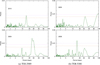 |
Fig. D.1 Periodograms of the WASP light curves. The dashed horizontal lines show the estimated 10% and 1%-likelihood false-alarm levels. |
Appendix E Joint modeling priors
Priors for the joint modeling of photometric and RV data.
Appendix F Limb darkening and photometric instrumental parameters
Fitted limb darkening parameters for the companions presented in this paper.
Fitted photometric instrumental parameters for the companions presented in this paper.
Appendix G Corner plots
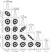 |
Fig. G.1 The corner plot for the Juliet results of TOI-2969. |
 |
Fig. G.2 The corner plot for the Juliet results of TOI-2989. |
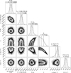 |
Fig. G.3 The corner plot for the Juliet results of TOI-5300. |
References
- Alibert, Y., Mordasini, C., & Benz, W. 2011, A&A, 526, A63 [NASA ADS] [CrossRef] [EDP Sciences] [Google Scholar]
- Aller, A., Lillo-Box, J., Jones, D., Miranda, L. F., & Barceló Forteza, S. 2020, A&A, 635, A128 [NASA ADS] [CrossRef] [EDP Sciences] [Google Scholar]
- Baraffe, I., Chabrier, G., & Barman, T. 2008, A&A, 482, 315 [NASA ADS] [CrossRef] [EDP Sciences] [Google Scholar]
- Bonfils, X., Delfosse, X., Udry, S., et al. 2013, A&A, 549, A109 [NASA ADS] [CrossRef] [EDP Sciences] [Google Scholar]
- Borsato, L., Degen, D., Leleu, A., et al. 2024, A&A, 689, A52 [NASA ADS] [CrossRef] [EDP Sciences] [Google Scholar]
- Boss, A. P. 1997, Science, 276, 1836 [Google Scholar]
- Bryan, M. L., Knutson, H. A., Howard, A. W., et al. 2016, AJ, 821, 89 [Google Scholar]
- Bryant, E. M., Bayliss, D., & Van Eylen, V. 2023, MNRAS, 521, 3663 [CrossRef] [Google Scholar]
- Burn, R., Schlecker, M., Mordasini, C., et al. 2021, A&A, 656, A72 [NASA ADS] [CrossRef] [EDP Sciences] [Google Scholar]
- Caldwell, D. A., Tenenbaum, P., Twicken, J. D., et al. 2020, RNAAS, 4, 201 [NASA ADS] [Google Scholar]
- Chabrier, G., & Debras, F. 2021, AJ, 917, 4 [Google Scholar]
- Collier Cameron, A., Wilson, D. M., West, R. G., et al. 2007, MNRAS, 380, 1230 [Google Scholar]
- Collins, K. 2019, in American Astronomical Society Meeting Abstracts, 233, 140.05 [Google Scholar]
- Cretignier, M., Dumusque, X., Allart, R., Pepe, F., & Lovis, C. 2020, A&A, 633, A76 [NASA ADS] [CrossRef] [EDP Sciences] [Google Scholar]
- Delamer, M., Kanodia, S., Canas, C. I., et al. 2024, AJ, 962, L22 [Google Scholar]
- ESA 1997, ESA Special Publication, 1200 [Google Scholar]
- Espinoza, N., & Jordán, A. 2015, MNRAS, 450, 1879 [Google Scholar]
- Espinoza, N., Kossakowski, D., & Brahm, R. 2019, MNRAS, 490, 2262 [Google Scholar]
- Evans, D. W., Eyer, L., Busso, G., et al. 2023, A&A, 674, A4 [NASA ADS] [CrossRef] [EDP Sciences] [Google Scholar]
- Eyer, L., Audard, M., Holl, B., et al. 2023, A&A, 674, A13 [NASA ADS] [CrossRef] [EDP Sciences] [Google Scholar]
- Fischer, D. A., & Valenti, J. 2005, AJ, 622, 1102 [Google Scholar]
- Foreman-Mackey, D. 2016, J. Open Source Softw., 1, 24 [Google Scholar]
- Fortney, J. J., Saumon, D., Marley, M. S., Lodders, K., & Freedman, R. S. 2006, AJ, 642, 495 [Google Scholar]
- Fortney, J. J., Marley, M. S., & Barnes, J. W. 2007, AJ, 659, 1661 [Google Scholar]
- Fortney, J. J., Dawson, R. I., & Komacek, T. D. 2021, J. Geophys. Res.: Planets, 126, e2020JE006629 [CrossRef] [Google Scholar]
- Gaia Collaboration (Vallenari, A., et al.) 2023, A&A, 674, A1 [NASA ADS] [CrossRef] [EDP Sciences] [Google Scholar]
- Gan, T., Wang, S. X., Wang, S., et al. 2023, AJ, 165, 17 [NASA ADS] [CrossRef] [Google Scholar]
- Garcia, L. J., Timmermans, M., Pozuelos, F. J., et al. 2022, MNRAS, 509, 4817 [Google Scholar]
- Gillon, M., Jehin, E., Magain, P., et al. 2011, in European Physical Journal Web of Conferences, 11, 06002 [Google Scholar]
- Grieves, N., Bouchy, F., Armstrong, D. J., et al. 2025, A&A, 693, A144 [NASA ADS] [CrossRef] [EDP Sciences] [Google Scholar]
- Grunblatt, S. K., Huber, D., Gaidos, E., et al. 2017, AJ, 154, 254 [Google Scholar]
- Guerrero, N. M., Seager, S., Huang, C. X., et al. 2021, ApJS, 254, 39 [NASA ADS] [CrossRef] [Google Scholar]
- Guillot, T., Santos, N. C., Pont, F., et al. 2006, A&A, 453, L21 [CrossRef] [EDP Sciences] [Google Scholar]
- Hacker, A., Díaz, R. F., Armstrong, D. J., et al. 2024, MNRAS, 532, 1612 [NASA ADS] [CrossRef] [Google Scholar]
- Hartman, J. D., Bakos, G. A., Torres, G., et al. 2009, AJ, 706, 785 [Google Scholar]
- Hartman, J. D., Bakos, G. A., Sato, B., et al. 2011, AJ, 726, 52 [Google Scholar]
- Hartman, J. D., Jordán, A., Bayliss, D., et al. 2020, AJ, 159, 173 [NASA ADS] [CrossRef] [Google Scholar]
- Hellier, C., Anderson, D. R., Collier Cameron, A., et al. 2010, AJ, 723, L60 [Google Scholar]
- Huang, C. X., Quinn, S. N., Vanderburg, A., et al. 2020a, AJ, 892, L7 [Google Scholar]
- Huang, C. X., Vanderburg, A., Pál, A., et al. 2020b, RNAAS, 4, 206 [NASA ADS] [Google Scholar]
- Husser, T.-O., Wende-von Berg, S., Dreizler, S., et al. 2013, A&A, 553, A6 [NASA ADS] [CrossRef] [EDP Sciences] [Google Scholar]
- Hut, P. 1981, A&A, 99, 126 [NASA ADS] [Google Scholar]
- Ida, S., & Lin, D. N. C. 2004, AJ, 616, 567 [Google Scholar]
- Ida, S., & Lin, D. N. C. 2005, AJ, 626, 1045 [Google Scholar]
- Jehin, E., Gillon, M., Queloz, D., et al. 2011, Messenger, 145, 2 [Google Scholar]
- Jenkins, J. M. 2002, AJ, 575, 493 [Google Scholar]
- Jenkins, J. M., Chandrasekaran, H., McCauliff, S. D., et al. 2010, SPIE Conf. Ser., 7740, 77400D [Google Scholar]
- Jenkins, J. M., Twicken, J. D., McCauliff, S., et al. 2016, SPIE Conf. Ser., 9913, 99133E [Google Scholar]
- Jenkins, J. M., Tenenbaum, P., Seader, S., et al. 2020, Kepler Data Processing Handbook: Transiting Planet Search, Kepler Science Document KSCI-19081-003, 9, Ed. J. M. Jenkins. [Google Scholar]
- Jensen, E. 2013, Tapir: A web interface for transit/eclipse observability, Astrophysics Source Code Library, record [record ascl:1306.007] [Google Scholar]
- Jordán, A., Hartman, J. D., Bayliss, D., et al. 2022, AJ, 163, 125 [NASA ADS] [CrossRef] [Google Scholar]
- Kanodia, S., Libby-Roberts, J., Canas, C. I., et al. 2022, AJ, 164, 81 [NASA ADS] [CrossRef] [Google Scholar]
- Kempton, E. M.-R., Bean, J. L., Louie, D. R., et al. 2018, PASP, 130, 114401 [CrossRef] [Google Scholar]
- Kipping, D. M. 2013a, MNRAS, 435, 2152 [Google Scholar]
- Kipping, D. M. 2013b, MNRAS, 434, L51 [Google Scholar]
- Kipping, D. M. 2014, MNRAS, 440, 2164 [CrossRef] [Google Scholar]
- Kovács, G., Zucker, S., & Mazeh, T. 2002, A&A, 391, 369 [Google Scholar]
- Kunimoto, M., Daylan, T., Guerrero, N., et al. 2022, ApJS, 259, 33 [NASA ADS] [CrossRef] [Google Scholar]
- Kurucz, R. L. 1993, SYNTHE spectrum synthesis programs and line data (Cambridge, Mass.: Smithsonian Astrophysical Observatory) [Google Scholar]
- Laughlin, G., Bodenheimer, P., & Adams, F. C. 2004, AJ, 612, L73 [Google Scholar]
- Lightkurve Collaboration (Cardoso, J. V. d. M., et al.) 2018, Astrophysics Source Code Library, [record ascl:1812.013] [Google Scholar]
- Martin, D. V., El-Badry, K., Hodžić, V. K., et al. 2021, MNRAS, 507, 4132 [CrossRef] [Google Scholar]
- Maxted, P. F. L., Anderson, D. R., Collier Cameron, A., et al. 2011, PASP, 123, 547 [NASA ADS] [CrossRef] [Google Scholar]
- Mayor, M., Marmier, M., Lovis, C., et al. 2011, arXiv e-prints, [arXiv:1109.2497] [Google Scholar]
- Mollière, P., van Boekel, R., Dullemond, C., Henning, T., & Mordasini, C. 2015, AJ, 813, 47 [Google Scholar]
- Mollière, P., van Boekel, R., Bouwman, J., et al. 2017, A&A, 600, A10 [Google Scholar]
- Mordasini, C., Alibert, Y., Benz, W., Klahr, H., & Henning, T. 2012a, A&A, 541, A97 [NASA ADS] [CrossRef] [EDP Sciences] [Google Scholar]
- Mordasini, C., Alibert, Y., Klahr, H., & Henning, T. 2012b, A&A, 547, A111 [NASA ADS] [CrossRef] [EDP Sciences] [Google Scholar]
- Müller, S., Ben-Yami, M., & Helled, R. 2020, AJ, 903, 147 [Google Scholar]
- Nissen, P. E. 2004, in Origin and Evolution of the Elements, eds. A. McWilliam, & M. Rauch, 154 [Google Scholar]
- Otegi, J. F., Bouchy, F., & Helled, R. 2020, A&A, 634, A43 [NASA ADS] [CrossRef] [EDP Sciences] [Google Scholar]
- Paegert, M., Stassun, K. G., Collins, K. A., et al. 2021, arXiv e-prints, [arXiv:2108.04778] [Google Scholar]
- Parc, L., Bouchy, F., Venturini, J., Dorn, C., & Helled, R. 2024, A&A, 688, A59 [NASA ADS] [CrossRef] [EDP Sciences] [Google Scholar]
- Pass, E. K., Winters, J. G., Charbonneau, D., et al. 2023, AJ, 166, 11 [NASA ADS] [CrossRef] [Google Scholar]
- Pecaut, M. J., & Mamajek, E. E. 2013, ApJS, 208, 9 [Google Scholar]
- Pinamonti, M., Sozzetti, A., Maldonado, J., et al. 2022, A&A, 664, A65 [NASA ADS] [CrossRef] [EDP Sciences] [Google Scholar]
- Pollacco, D., Skillen, I., Cameron, A., et al. 2006, PASP, 118, 1407 [NASA ADS] [CrossRef] [Google Scholar]
- Pollack, J. B., Hubickyj, O., Bodenheimer, P., et al. 1996, Icarus, 124, 62 [NASA ADS] [CrossRef] [Google Scholar]
- Prša, A., Harmanec, P., Torres, G., et al. 2016, AJ, 152, 41 [Google Scholar]
- Queloz, D., Mayor, M., Udry, S., et al. 2001, Messenger, 105, 1 [Google Scholar]
- Ribas, I., Reiners, A., Zechmeister, M., et al. 2023, A&A, 670, A139 [NASA ADS] [CrossRef] [EDP Sciences] [Google Scholar]
- Ricker, G. R., Winn, J. N., Vanderspek, R., et al. 2014, JATIS, 1, 014003 [NASA ADS] [Google Scholar]
- Riello, M., De Angeli, F., Evans, D. W., et al. 2021, A&A, 649, A3 [NASA ADS] [CrossRef] [EDP Sciences] [Google Scholar]
- Safonov, B. S., Lysenko, P. A., & Dodin, A. V. 2017, Astron. Lett., 43, 344 [NASA ADS] [CrossRef] [Google Scholar]
- Santos, N. C., Mayor, M., Naef, D., et al. 2002, A&A, 392, 215 [NASA ADS] [CrossRef] [EDP Sciences] [Google Scholar]
- Santos, N. C., Israelian, G., & Mayor, M. 2004, A&A, 415, 1153 [NASA ADS] [CrossRef] [EDP Sciences] [Google Scholar]
- Santos, N. C., Sousa, S. G., Mortier, A., et al. 2013, A&A, 556, A150 [NASA ADS] [CrossRef] [EDP Sciences] [Google Scholar]
- Sarkis, P., Mordasini, C., Henning, T., Marleau, G. D., & Mollière, P. 2021, A&A, 645, A79 [NASA ADS] [CrossRef] [EDP Sciences] [Google Scholar]
- Saumon, D., Chabrier, G., & van Horn, H. M. 1995, ApJS, 99, 713 [NASA ADS] [CrossRef] [Google Scholar]
- Schlegel, D. J., Finkbeiner, D. P., & Davis, M. 1998, AJ, 500, 525 [NASA ADS] [CrossRef] [Google Scholar]
- Seager, S., & Mallen-Ornelas, G. 2003, AJ, 585, 1038 [Google Scholar]
- Sestovic, M., Demory, B.-O., & Queloz, D. 2018, A&A, 616, A76 [NASA ADS] [CrossRef] [EDP Sciences] [Google Scholar]
- Smith, J. C., Stumpe, M. C., Van Cleve, J. E., et al. 2012, PASP, 124, 1000 [Google Scholar]
- Sneden, C. A. 1973, PhD Thesis, University of Texas, Austin, USA [Google Scholar]
- Sousa, S. G. 2014, in Determination of Atmospheric Parameters of B, eds. E. Niemczura, B. Smalley, & W. Pych, 297 [Google Scholar]
- Sousa, S. G., Santos, N. C., Adibekyan, V., Delgado-Mena, E., & Israelian, G. 2015, A&A, 577, A67 [NASA ADS] [CrossRef] [EDP Sciences] [Google Scholar]
- Sousa, S. G., Santos, N. C., Israelian, G., Mayor, M., & Monteiro, M. J. P. F. G. 2007, A&A, 469, 783 [NASA ADS] [CrossRef] [EDP Sciences] [Google Scholar]
- Sousa, S. G., Adibekyan, V., Delgado-Mena, E., et al. 2021, A&A, 656, A53 [NASA ADS] [CrossRef] [EDP Sciences] [Google Scholar]
- Speagle, J. S. 2020, MNRAS, 493, 3132 [Google Scholar]
- Stassun, K. G., & Torres, G. 2016, AJ, 152, 180 [Google Scholar]
- Stassun, K. G., & Torres, G. 2021, AJ, 907, L33 [Google Scholar]
- Stassun, K. G., Collins, K. A., & Gaudi, B. S. 2017, AJ, 153, 136 [Google Scholar]
- Stassun, K. G., Corsaro, E., Pepper, J. A., & Gaudi, B. S. 2018, AJ, 155, 22 [Google Scholar]
- Stassun, K. G., Oelkers, R. J., Paegert, M., et al. 2019, AJ, 158, 138 [Google Scholar]
- Stumpe, M. C., Smith, J. C., Van Cleve, J. E., et al. 2012, PASP, 124, 985 [Google Scholar]
- Stumpe, M. C., Smith, J. C., Catanzarite, J. H., et al. 2014, PASP, 126, 100 [Google Scholar]
- Thommes, E. W., Matsumura, S., & Rasio, F. A. 2008, Science, 321, 814 [NASA ADS] [CrossRef] [Google Scholar]
- Thompson, C. V. 1990, Annu. Rev. Mater. Res., 20, 245 [Google Scholar]
- Tokovinin, A. 2018, PASP, 130, 035002 [Google Scholar]
- Torres, G., Winn, J. N., & Holman, M. J. 2008, AJ, 677, 1324 [Google Scholar]
- Torres, G., Andersen, J., & Giménez, A. 2010, A&ARev., 18, 67 [Google Scholar]
- Tsantaki, M., Sousa, S. G., Adibekyan, V. Z., et al. 2013, A&A, 555, A150 [NASA ADS] [CrossRef] [EDP Sciences] [Google Scholar]
- Twicken, J. D., Catanzarite, J. H., Clarke, B. D., et al. 2018, PASP, 130, 064502 [Google Scholar]
- Ulmer-Moll, S., Lendl, M., Gill, S., et al. 2022, A&A, 666, A46 [NASA ADS] [CrossRef] [EDP Sciences] [Google Scholar]
- Vines, J. I., Jenkins, J. S., Acton, J. S., et al. 2019, MNRAS, 489, 4125 [NASA ADS] [CrossRef] [Google Scholar]
- Vorobyov, E. I., & Basu, S. 2008, AJ, 676, L139 [Google Scholar]
- Wright, J. T., Marcy, G. W., Howard, A. W., et al. 2012, AJ, 753, 160 [Google Scholar]
See the NASA Exoplanet Archive exoplanetarchive.ipac.caltech.edu, accessed 20 January 2025.
Mass precision <25%.
The spectral types are defined by the effective temperatures, as listed in Table 5 of Pecaut & Mamajek (2013).
This radius range also includes M dwarfs, but we vetted the data to exclude stellar companions.
The last version, ARES v2, can be downloaded at https://github.com/sousasag/ARES
All Tables
Fitted photometric instrumental parameters for the companions presented in this paper.
All Figures
|
Fig. 1 HR diagram of all Gaia DR3 nearby stars with parallax π ≥ 10 mas, where the colors indicate log(g). The three stars presented in this work are overplotted and visible on the main sequence. |
| In the text | |
|
Fig. 2 Phase-folded Gaia photometric data. Colored points indicate the different Gaia wave bands. The black points show the TESS data, binned in intervals of 1/1000 of the period. The errors in the Gaia data are corrected following Evans et al. (2023) by adding an error in quadrature as a function of the magnitude. Long-period signals above 0.01% false alarm probability (FAP) are subtracted, and the errors are scaled by the ratio of the standard deviation before and after signal subtraction. |
| In the text | |
|
Fig. 3 Overlay of TOI-2969’s orbital solution with CORALIE RV observations, with residuals shown in the lower panel (RMS of 23 m/s). |
| In the text | |
|
Fig. 4 Orbital solution for TOI-2989 alongside its CORALIE RV data. |
| In the text | |
|
Fig. 5 Orbital solution for TOI-5300 superimposed on CORALIE RV data, with residuals plotted in the lower panel (RMS of 68 m/s). |
| In the text | |
|
Fig. 6 Phase-folded TESS light curve of TOI-2969. The Juliet fit is shown as a black line, while TESS data is plotted in light blue in the lower panel. The upper panels feature ground-based follow-up photometric observations from LCO-SAAO, LCO-CTIO, TRAPPIST-South, El Sauce, SUTO, and PEST. Data points with black-edged markers indicate 10-minute bins, except for LCO-SAAO (g′) observations, which are binned by 15 minutes. If the dilution D is fitted, it is indicated per light curve, otherwise, it is set to 1. |
| In the text | |
|
Fig. 7 Phase-folded TESS light curve of TOI-2989. The Juliet fit is shown as a black line, while TESS data is plotted in light blue in the lower panel. The upper panels feature ground-based follow-up photometric observations from El Sauce and TRAPPIST-South. Data points with black-edged markers indicate 10-minute bins. |
| In the text | |
|
Fig. 8 Phase-folded TESS light curve for TOI-5300. The Juliet model fit is depicted as a black line, while TESS data shown in light blue in the lower panel. The upper panels include ground-based photometric observations from LCO-CTIO, LCO-HAL, TRAPPIST-South, and Brierfield. Data points with black-edged markets indicate 10-minute bins for TESS, Brierfield, and TRAPPIST-South, 15-minute intervals for LCO-CTIO and LCO-HAL (i′), and 30-minute intervals for LCO-HAL(g′). |
| In the text | |
|
Fig. 9 Overview of the presented companions (encircled in red) compared to known planets from the PlanetS catalog (extended from Otegi et al. (2020); Parc et al. (2024), updated August 2024). The data are color coded by planetary radii. The histogram at the top shows the relative occurrence of the transiting gas giants with masses ranging from 0.1 to 13 MJup. The low-mass star regime remains relatively poorly populated; our three mass characterizations contribute to this population. |
| In the text | |
|
Fig. A.1 Speckle observations from SOAR. |
| In the text | |
|
Fig. A.2 SAI speckle interferometry - TOI-5300, UTC 2023 September 30 |
| In the text | |
|
Fig. B.1 The spectral energy distributions (SEDs). Red symbols represent the observed photometric measurements, and the horizontal bars represent the effective width of the passband. Blue symbols are the model fluxes from the best-fit PHOENIX atmosphere model (black). The insets show the absolute flux-calibrated Gaia spectrophotometry as a gray swathe overlaid on the model (black). |
| In the text | |
|
Fig. C.1 The Lomb-Scargle periodogram of the Gaia DR3 photometric observations. The observations are filtered based on flags for photometry and variability. The false alarm probability (FAP) levels are overplotted for the combined data sets. |
| In the text | |
|
Fig. D.1 Periodograms of the WASP light curves. The dashed horizontal lines show the estimated 10% and 1%-likelihood false-alarm levels. |
| In the text | |
|
Fig. G.1 The corner plot for the Juliet results of TOI-2969. |
| In the text | |
|
Fig. G.2 The corner plot for the Juliet results of TOI-2989. |
| In the text | |
|
Fig. G.3 The corner plot for the Juliet results of TOI-5300. |
| In the text | |
Current usage metrics show cumulative count of Article Views (full-text article views including HTML views, PDF and ePub downloads, according to the available data) and Abstracts Views on Vision4Press platform.
Data correspond to usage on the plateform after 2015. The current usage metrics is available 48-96 hours after online publication and is updated daily on week days.
Initial download of the metrics may take a while.