| Issue |
A&A
Volume 700, August 2025
|
|
|---|---|---|
| Article Number | A192 | |
| Number of page(s) | 14 | |
| Section | Interstellar and circumstellar matter | |
| DOI | https://doi.org/10.1051/0004-6361/202554839 | |
| Published online | 19 August 2025 | |
Ammonia in the hot core W51-IRS2: Maser line profiles, variability, and saturation
1
Max-Planck-Institut für Radioastronomie,
Auf dem Hügel 69,
53121
Bonn,
Germany
2
Astronomy Department, Faculty of Science, King Abdulaziz University,
PO Box 80203,
Jeddah
21589,
Saudi Arabia
3
Xinjiang Astronomical Observatory, Chinese Academy of Sciences,
830011
Urumqi,
PR China
4
Purple Mountain Observatory (PMO) and Key Laboratory of Radio Astronomy, Chinese Academy of Sciences,
10 Yuanhua Road,
Nanjing
210023,
PR China
5
National Radio Astronomy Obsrevatory,
520 Edgemont Road,
Charlottesville,
VA
22903-2475,
USA
★ Corresponding author.
Received:
28
March
2025
Accepted:
19
June
2025
Abstract
W51-IRS2 is known to be one of the most prolific sources of interstellar ammonia (NH3) maser lines. So far, however, many of these inversion lines have rarely been studied. Here we report spectrally resolved line profiles for the majority of detected features and provide information on the variability of these maser components between 2012 and 2023. This includes the first tentative detection of a (J, K) = (5, 2) maser in the interstellar medium and the first tentative detection of a (6,4) maser in W51-IRS2. Furthermore, we report for the first time NH3 (9,6) maser emission below local standard of rest velocities of 50 km s–1 in this source as well as double maser features occasionally seen in other transitions. The detected maser lines strongly indicate vibrational pumping by ≈10 μm photons, which must be abundant due to the high kinetic temperature (≈300 K) of the ammonia emitting gas. The detection of vibrationally excited NH3, suggesting a vibrational excitation temperature consistent with the kinetic one, and a comparison with measured SiO line profiles, are also presented. For the (10,7) line, we find a tentative correlation between flux density and line width compatible with unsaturated maser emission. The velocity drift of the so-called 45 km s–1 maser features, reported to be +0.2 km s–1 yr–1 between 1996 and 2012, has either slowed down to values <0.1 km s–1 or has entirely disappeared. In 2023, the component is only seen in ammonia inversion lines that are located at least 800 K above the ground state. The other features have faded. Possible scenarios explaining this phenomenon are discussed.
Key words: ISM: clouds / ISM: molecules / ISM: individual objects: W51
© The Authors 2025
 Open Access article, published by EDP Sciences, under the terms of the Creative Commons Attribution License (https://creativecommons.org/licenses/by/4.0), which permits unrestricted use, distribution, and reproduction in any medium, provided the original work is properly cited.
This article is published in open access under the Subscribe to Open model.
Open Access funding provided by Max Planck Society.
1 Introduction
Ammonia (NH3) provides unique opportunities to trace molecular cloud excitation up to temperatures of ≳1000K (e.g., Wilson et al. 2006) by observing its inversion transitions within a very limited frequency interval (20–45 GHz). Dozens of inversion lines can be detected in this frequency range, provided kinetic temperatures and column densities are high enough. Warmer conditions are characteristic of “hot cores”, dense molecular condensations near sites of massive star formation that are chemically affected by dust grain mantle evaporation through sudden irradiation by an intense UV radiation field from short-lived OB stars (e.g., Genzel et al. 1982; Henkel et al. 1987; Walmsley et al. 1987; Brown et al. 1988; Charnley et al. 1992; Caselli et al. 1993; Wakelam et al. 2005; Bisschop et al. 2007; Garrod et al. 2013). In such environments large numbers of hydrogenated molecules may enter the gas phase, with ammonia and water vapor among the most notable species. The warm dense clumps are characterized by temperatures of Tkin> 100 K, X(NH3) = N(NH3)/N(H2) ≈ 10–5…–6, and source averaged ammonia column densities in excess of 1018 cm–2 (e.g., Mauersberger et al. 1987).
Not all of the ammonia inversion lines are thermally excited. (J, K) = (3,3) maser emission was first detected by Wilson et al. (1982) toward the star-forming region W33. This maser is readily explained by the fact that the two lowest K-ladders of the symmetric ortho-NH3 molecule, those for K = 0 and 3, are radiatively connected and that the K=0 ladder is the one devoid of inversion doublets (it is characterized instead by single rotational states). The single (0,0) state, the important and usually well-populated ground state, is collisionally connected to only the upper level of the (3,3) inversion doublet, which inverts the populations of the two (3,3) levels under specific physical conditions (e.g., Walmsley & Ungerechts 1983).
By 18 years ago, several maser lines had already been identified (for instance Guilloteau et al. 1983; Gaume et al. 1996; Madden et al. 1986; Mauersberger et al. 1986a, 1987, 1988; Cesaroni et al. 1992; Mangum & Wootten 1994; Beuther et al. 2007), with detections not only including the (3,3) line of 14NH3 but also that of 15NH3 (Mauersberger et al. 1986b; Schilke et al. 1991). Other inversion doublets were also found to be masing. The numerous lines detected during the last decade (e.g., Henkel et al. 2013; Mills et al. 2018; Mei et al. 2020; Yan et al. 2022a,b, 2024), first toward W51 and then also toward SgrB2 and other massive star-forming regions, often include lines of ortho-NH3 (K = 0, 3, 6, 9, …). However, many transitions of para-NH3 (K = 1, 2, 4, 5, 7, 8, …) were also found. To date, maser transitions have been detected in more than 30 different ammonia inversion lines (for a list, see Table A.1 in Yan et al. 2024). These are usually found at levels hundreds of Kelvins above the ground state, with the (J, K) = (12,12) transition at ≈1450 K reaching the highest value. With the exception of the (1,1) (Gaume et al. 1996), (2,2) (Mills et al. 2018), (3,3) (Wilson et al. 1982, (5,5) (Cesaroni et al. 1992), (6,6) (Beuther et al. 2007), (7,7) (9,9), and (12,12) (Henkel et al. 2013) inversion doublets, the maser lines originate from non-metastable levels, requiring extremely high densities (≳108 cm–3) and/or intense infrared radiation fields to become populated. While the (3,3) maser lines are readily reproduced by large velocity gradient (LVG) radiative transfer models, explanations for the other masers are difficult to attain. These possibly require a quantitative understanding of vibrational excitation, which is a problem, because until recently collisional rates were only available up to the (6,6) state of the ground vibrational level and because IR line overlaps with transitions from other molecular species might also play a role. Quite recently, Demes et al. (2023) published collision rates for ortho-NH3 up to (J, K) = (10,9), including the (9,6) inversion doublet and para NH3 up to (10,10), but without the (10,7) transition, while Loreau et al. (2023) reported collision rates for all hyperfine levels up to J = 4.
The detection of 11 new maser lines in outer space, all of them from NH3 toward the Galactic hot core W51-IRS2 (D ≈ 5.0±0.3 kpc; Sato et al. 2010) and additional masers previously not seen in this specific source (Henkel et al. 2013) led to a total of 21 detected ammonia maser transitions alone in this hot core, all of them representing inversion lines. For a radio continuum image, see Fig. 1, taken from Ginsburg et al. (2016). For the detailed distribution of quasi-thermal ammonia emission, see Fig. 2. The single-dish study by Henkel et al. (2013) was complemented by observations with a much higher angular resolution (≈0.″; Goddi et al. 2015) to localize some of the most characteristic maser features and by Zhang et al. (2022, 2024b), who measured maser lines during five epochs in early 2020 with the 65-m Tian Ma Radio Telescope (TMRT) and the Jansky Very Large Array (JVLA).
Here, we provide follow-up observations of these so far poorly studied maser lines, presenting for many of these features spectrally resolved line shapes and information on their variability over a timescale of ≳ 10 yr. Complementary measurements of an ammonia line connecting two vibrationally excited energy levels and of SiO J = 1→0 maser lines are also addressed. Sect. 2 describes the measurements and Sect. 3 introduces the observed data, while a deeper analysis of measured profiles is given in Sect. 4. Finally, Sect. 5 summarizes the main results.
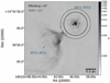 |
Fig. 1 Jansky Very Large Array continuum map of the W51 region at 14.5 GHz (image taken from Ginsburg et al. 2016; synthesized beam size: 0.″). W51d is associated with the northwestern hotspot, W51-IRS2, while the more extended bright region to the southeast is W51-IRS1. Our Effelsberg beam size of ≈40″ (the inner circle) encompasses the entire IRS2 region, but is small enough to exclude IRS1. The slightly larger circle, corresponding to 55″, refers to the beam size of the Tian Ma Radio telescope near Shanghai. |
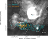 |
Fig. 2 Overlay of the 25 GHz continuum emission (gray scale and white contours) and the integrated intensities of the quasi-thermal (6,6) and (10,10) lines of ammonia (taken from Goddi et al. 2015). The (6,6) contours show the elongated dense molecular environment at the southern boundary of the H II region W51d. The location of main molecular hotspots, W51N4, W51d2, W51N2, and W51-North (from west to east), are indicated. For more details, see Goddi et al. (2015). |
2 Observations
2.1 Ammonia (NH3) at K-band (λ ≈ 1.3 cm)
New data were taken at several epochs between January and May 2013 and then again in February 2017, January and February 2018, January 2020, and several times between March 2022 and May 2023 with the 100-m telescope at Effelsberg1 near Bonn, Germany. For earlier measurements also playing a role in this work, see Henkel et al. (2013). The chosen position was as in Henkel et al. (2013)  ,
,  , about 4.″7 north of W51d2 and
  northwest of the main source W51-North (see Fig. 5 of Zhang et al. 2024a, our Fig. 2 and Sect. 4.6). At the line frequencies observed (18–26 GHz), the beam size is 50″–35″. Intensity scales were established with a noise diode by continuum cross scans toward 3C 286 and NGC 7027. Flux densities were taken from Ott et al. (1994), also accounting for a 0.5% yr–1 secular decrease in the case of NGC 7027, and for gain variations of the telescope as a function of elevation2. 1923+210 and 2145+06 were used as pointing sources. The pointing accuracy was better than 10″. For maser sources much more compact than the beam size, line shapes are not affected by pointing errors.
During the measurements in 2013, the front-end was a dual channel (including the two orthogonal linear polarizations) cooled primary focus HEMT (Hot Electron Mobility Transistor) receiver with a Tsys equivalent to ≈65 Jy per channel. In 2017 and later, a secondary focus 1.4cm two horn system was used covering left- and right-hand circular polarization with a Tsys equivalent to ≈55 Jy.
For the earlier measurements in 2013, a fast Fourier transform spectrometer (FFTS) was employed with a bandwidth of 100 MHz and 32 768 channels per linear polarization, implying channel widths of order 0.04 km s–1. During some of the later measurements in 2017 to 2023, the full 8 GHz wide band of the secondary focus receiver could be covered simultaneously by several FFTS spectrometers. For each circular polarization this resulted in four partially overlapping spectra with 2.5 GHz bandwidth and 65 536 spectral channels, centered at 19.25, 21.15, 22.85, and 24.75 GHz and yielding channel widths of order 0.5 km s–1. In 2022 and 2023, a high resolution backend with 65 536 channels and a bandwidth of 300 MHz was occasionally employed, providing a channel width of 0.07 km s–1 at 18.5 GHz. Spectral resolutions are slightly coarser than the respective channel widths, by 16% (see Klein et al. 2012) for the spectra taken after 2013.
All data for the lines relevant for this article (see Table 1) were taken in a position switching mode, employing scans of 5 min total (on + off) duration and alternating offset positions 15′ east and west. For the calibration of the data taken in 2013, narrow band (≈500 MHz) continuum scans were taken to account for frequency-dependent variations in the noise diode signal. For the 8 GHz wide spectra, “spectroscopic” pointings covering the entire band were obtained with individual spectral widths of ≈300 MHz. The wide (≈2.5 GHz) spectral subbands were split into smaller subbands of size ≈300 MHz, accounting for atmospheric attenuation and elevation dependent telescope gain corrections. The calibration uncertainties are estimated to be ±15% after accounting for the elevation dependent gain of the 100-m telescope.
Studied ammonia lines showing at least potential maser features.
2.2 Silicon monoxide (SiO) with the 100-m telescope
In April 2014, we also searched for J = 1→0 SiO maser emission in the first and second vibrationally excited levels (υ =1 and 2) toward W51-IRS2. As in the case of ammonia, position switching with alternating offsets in east-west directions was used. These measurements were carried out with a secondary focus receiver with a Tsys equivalent of ≈300 Jy. For these measurements, an FFTS with 100 MHz bandwidth and 32 768 channels has been employed. The beam size was 22″. Pointing was based on measurements of the nearby source 1923+210 and was found to be accurate within 5″–7″. K3-50A was used as calibration source. We adopted a flux density of 6.9±1.0jy for K3-50A (Howard et al. 1997, their Fig. 2). With the given flux density error and in view of the large difference in declination between K3-50A and W51-IRS2, we estimate a calibration uncertainty of ± 25% after accounting for elevation dependent telescope gain variations.
2.3 Ammonia (NH3) with the 12-m APEX telescope
We also observed emission from a line of vibrationally excited ammonia toward W51-IRS2, selecting the ν2 = 1, (0,0) → (1,0) transition at 466.244GHz. The measurements were carried out in 2013, April, using APEX3 (Atacama Pathfinder Experiment; Güsten et al. 2006), located on the Chajnantor plateau in Chile. The front-end was FLASH+ (First Light APEX Submillimeter Heterodyne, Klein et al. 2014), a dual frequency SiS mixer system operating simultaneously, on orthogonal polarizations, in the 345 GHz and 460GHz atmospheric windows.
The beam size was 13″. Observed were the CO J = 3→2 line at ≈345.796 GHz, its image frequency at 333.796 GHz, as well as ammonia at ≈466.245 GHz and its image frequency at 478.245 GHz. Each of these frequencies were covered with two 2.5 GHz wide spectra, one offset to the blue and the other one to the red side, including an overlapping region of width ≈0.7 GHz centered at the line frequency.
The measurements were carried out in cold clear weather with precipitable water vapor measuring ≈0.65 mm and system temperatures of Tsys ≈ 200 and 500 K at 345 GHz and 466 GHz, respectively, on a  scale. Pointing accuracy was established by measurements of Saturn. The resulting antenna temperatures,
  , were converted to main beam brightness temperatures of
  using a forward hemisphere efficiency of Feff = 0.95 and a main beam efficiency of Beff = 0.60. The conversion factor between the
  temperature and the flux density scale is ≈50 Jy/K.
3 Results
3.1 General aspects
Making use of the available 8 GHz wide Effelsberg spectra, we checked systematically all 49 ammonia inversion transitions with rotational quantum numbers up to J = 16 that can be found in the observed frequency interval between 18 and 26 GHz. Figs. A.1 to A.44 in Appendix A show the detected NH3 inversion lines in the ground vibrational level with at least tentatively detected maser features. 20 lines following rising quantum number J from J = 5 to 11 are included, with a spectrum from 2012 (also shown by Henkel et al. 2013) at the bottom left and the most recent ones in the upper right. For the particularly frequently measured (9,6) and (10,7) lines, new spectra are presented exclusively. Characteristic channel widths are 0.5–1.0 km s–1. While a comparison of spectra from 2012 (also published by Henkel et al. 2013), 2013, 2017, 2018, 2020, 2022, and 2023 provides a view on long-term variability, we also present (if lines are strong enough) data at five epochs within a six day interval between January 24, 2018, and February 1, 2018, to trace variability on short timescales. Covering slightly larger time intervals, we also show spectra from five monitoring epochs between April 11 and May 4, 2023. Furthermore, a large number of high-spectral-resolution (J, K) = (9,6) and (10,7) profiles are presented, taken in 2022 and 2023, while a few high resolution spectra from other inversion lines are also obtained. Results from Gaussian fits are given in Tables B.1 to B.19 of Appendix B.
3.2 Use of the quasi-thermal lines
While this article focuses on maser features, the quasi-thermal emission centered near VLSR = 60 km s–1 (here and elsewhere we use local standard of rest velocities) is useful because it arises from relatively large volumes and may thus not show significant variability. As a consequence the thermal features can be used as an additional means to calibrate spectra, providing an independent check with respect to the calibration methods outlined in Sect. 2.1. Comparing our quasi-thermal features with those reported by Mauersberger et al. (1987; their Table 1, 1.4 K in units of main beam brightness temperature correspond to about 1 Jy), which were also obtained with the Effelsberg 100-m telescope, agreement is reasonably good in the case of the (5,4), (7,6), (7,7), (9,7), and (10,8) lines. Furthermore, our detected 60 km s–1 feature of the (6,2) line is consistent with the upper limit provided by Mauersberger et al. (1987). For the (6,6) line, our 60 km s–1 feature is consistent with that published by Henkel et al. (2013). In the case of the (7,5) line, the quasi-thermal feature reaches levels of 0.05–0.08 Jy, slightly below the 0.1 Jy reported by Mauersberger et al. (1987). A similar situation is encountered in the case of the (8,6) line, while our calibration yields quasi-thermal (9,8) and (11,9) features about a factor of two weaker than those reported by Mauersberger et al. (1987). To summarize, our calibrated spectra provide flux density scales that have a tendency to yield smaller values than those reported by Mauersberger et al. (1987), ranging from good agreement in most cases down to a factor of two below the previously reported peak intensities in the most extreme cases. Discrepancies tend to appear in the lines with highest excitation above the ground state, i.e., in those cases in which the quasi-thermal emission centered near VLSR = 60 km s–1 is showing a particularly compact spatial distribution (Goddi et al. 2015). Interferometric data (Fig. 2 and again Goddi et al. 2015) indicate sizes of ≈0.5×0.1 and ≈0.1×0.1 lightyears2 for the (6,6) and (9,9) lines and suggest even smaller sizes for the non-metastable inversion lines, so that variability within a decade may well be possible. Nevertheless it remains open whether the observed discrepancies in peak intensity are caused by pointing errors, calibration uncertainties or by real changes in the emission profile. To stay on the conservative side, in the following it is assumed that all discrepancies in the time interval between 2012 and 2023 are due to calibration uncertainties.
3.3 New maser lines
Searching for new maser transitions not yet seen in W51-IRS2 or, even better, not yet seen anywhere in the interstellar medium, we have analyzed the 49 inversion lines mentioned in Sect. 3.1 and have found two candidates. The first is the (5,2) transition (Fig. A.1). While apparently not being present in 2012, 2017 and 2020, there is a feature off the quasi-thermal VLSR = 60 km s–1 component in late April and early May, 2023, not being present in early April and late May 2023. (5,2) maser emission has to our knowledge never been reported before (see, e.g., Table A.1 in Yan et al. 2024). Another maser candidate is the (6,4) inversion line (Figs. A.11 and A.12), which is seen throughout April and early May, 2023, disappearing like the (5,2) feature in late May. Velocities are in both cases VLSR ≈ 57 km s–1. Note that a (6,4) maser was reported before by Mei et al. (2020) in SgrB2(N). Signal-to-noise ratios for both spectral features, in the (5,2) and (6,4) lines, are such that we rate them as tentatively detected following Figs. A.1, A.11 and A.12. However, the averages of the spectra taken in April and May 2023 (Fig. 3) show those narrow features more convincingly with signal-to-noise ratios of 3.5 and 10 (Tables B.7 and B.10) that are most readily interpreted in terms of maser emission. While 10σ may appear to be high for a tentative detection, we should keep in mind that the feature is heavily blended by the comparatively broad quasi-thermal feature centered at ≈60 km s–1. The (7,3) maser, not covered by Henkel et al. (2013) and being first detected by Zhang et al. (2022), is confirmed and demonstrated to be present since at least 2018. This implies that during the last decade no strong new maser line has appeared with the potential exception of the (7,3) transition.
3.4 The maser families
Henkel et al. (2013) distinguished between four maser families, those measured near 45 km s–1 (or at slightly higher velocities), 54 km s–1, and 57 km s–1 and the (9,6) maser line, which is unique with respect to its strength and its wide velocity range. We trace five transitions that definitely show the 57 km s–1 maser component (the (5,2), (5,3), (5,4), (6,3), and (6,4) lines), and six host features near 45 km s–1 (the (6,6), (7,6), (7,7), (8,6), (10,9), and (11,9) transitions). In these cases occasionally even two velocity components are found of which the lower velocity feature is addressed in Sect. 3.4.1. The phenomenon is discussed in more detail in Sect. 3.4.4. Eight transitions emit maser emission near 54 km s–1, the (6,2), (7,3), (7,4), (7,5), (8,5), (9,7), (9,8), and (10,7) lines. In the (5,4) line a weak feature accompanying the main 57 km s–1 maser component is also seen near 54 km s–1 (Fig. A.6). The maser families are summarized in Table 2.
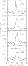 |
Fig. 3 Averaged NH3 spectra from April and May 2023. Channel widths are 0.60, 0.55, 0.61, and 0.56 km s–1 from top to bottom, respectively. |
NH3 maser families in W51-IRS2.
3.4.1 Variability on comparatively long timescales
The first question is related to variability and whether it is correlated, in the sense that all the masers in Figs. A.1 to A.44 change their flux densities in a similar manner, or whether at least those belonging to a specific maser family are correlated. Unlike in the case of the comparatively broad quasi-thermal profiles, maser lines tend to be narrow so that, to be independent from the chosen channel spacing, integrated intensities will be compared. For the moment neglecting the (9,6) line and starting with the lowest velocity component, that near 45 km s–1, we see an almost general decline in all six traced transitions. Flux densities from April 2012 to early 2018 decrease by factors of order 40, 5, 1.0, 10, 10 and 50 for the (6,6), (7,6), (7,7), (8,6), (10,9), and (11,9) transitions, respectively. Averaging our (6,6) profiles from 2023 April and May does not yield a detection with a 3σ value of 0.1 Jy for a channel spacing of 0.46 km s–1. For the eight lines near 54 km s–1 we obtain a decline by a factor of 4 for the (6,2) line, little change in the (7,3), (7,4), (7,5), and (8,5) transitions, a drop by a factor of approximately 1.5 in the (9,7) and (9,8) lines and a strong increase in the (10,7) line, by a factor of ≈15. In the case of our three transitions already previously known to belong to the 57 km s–1 maser family, the changes are not large. Flux densities tend to stay constant in the case of the (5,3), (5,4), and (6,3) lines between 2012 and 2018. The (5,2) and (6,4) lines are too weak to check variability.
For the time interval between 2018 and 2023, emission from the VLSR ≈ 45 km s–1 component is weak. While the (7,7) feature remains strong till 2020, after 2020 this maser component is only detected in the (7,6), (8,6) and (11,9) transitions. The 54 km s–1 feature shows quite different trends. The (7,3), (7,4), (7,5), (9,7), and (10,7) transitions keep approximately their intensities. The (6,2) feature is barely seen in 2023 (Fig. 3) and the (8,5) line intensity drops by a factor of approximately three between 2018 and 2020 and remains weak (and constant) till the end of our monitored time interval (Fig. 4). The (9,8) transition is weak but still present throughout this time period (Fig. 4).
While more details will be given below, the (9,6) line spectra with coarse velocity resolution (Figs. A.29 and A.30) show a drift of the strongest velocity component toward lower velocities from almost 55 to a little above 53 km s–1 between 2013 and 2023. Its ≈60 km s–1 component shows a line shape very similar to the quasi-thermal features seen in other inversion lines. However, this VLSR ≈ 60 km s–1 component is ≈50 times stronger than the corresponding features in the (9,7) and (9,8) lines and thus far too strong to be of quasi-thermal origin. Near the end of our monitoring time interval, emission is also seen at velocities <50 km s–1.
3.4.2 The most likely pumping scheme
From this admittedly superficial analysis of variability we can already conclude that the different maser families are not directly connected. Even within the families, strong differences in variability may occur, but only in one case, that of the 54 km s–1 component, we find both masers with clearly decreasing and increasing flux densities. Henkel et al. (2013) and Goddi et al. (2015) interpreted maser emission detected at the same radial velocity, typically encountered in (J, K) and in (J + 1, K) transitions, as caused by infrared pumping. Because of similar parities (see, e.g., Fig. 10 of Henkel et al. 2013) in adjacent inversion doublets within a given K-ladder, spontaneous decay through rotational transitions from a (J + 1, K) to a (J, K) inversion doublet leads from the upper state in the (J + 1, K) to the lower state in the (J, K) doublet and vice versa. Thus population inversion in the upper inversion doublet would lead to anomalous cooling of the level populations in the lower doublet, leading for example with inversion in the (9,7) to anti-inversion in the (8,7) and once again to inversion in the (7,7) doublets. To obtain population inversion and maser emission in adjacent (ΔJ = 1, ΔK = 0) doublets, vibrational excitation is required through ≈ 10 μm photons, abundant in the ≈ 300 K environment of W51-IRS2 (Mauersberger et al. 1987). Then parities are reversed twice, from plus to minus and back to plus or from minus to plus and then back to minus, first due to radiative excitation by infrared photons and second due to rapid spontaneous decay. In this case, inversion in the upper vibrational ground state doublet also supports inversion in the lower one.
Our maser lines include a number of adjacent (J, K)–(J + 1, K) transitions in a given K-ladder, the (5,2) and (6,2), the (9,7) and (10,7), and the (10,9) and (11,9) doublets, the (5,3), (6,3), and (7,3) as well as the (5,4), (6,4), and (7,4) triplets, and the (6,6), (7,6), (8,6), and (9,6) quadruplet. Thus more than a dozen of our 20 monitored maser lines are involved. Furthermore we may look for a connection between the (7,7) and (9,7) lines even though the (8,7) line did not reveal any masing component at a ≳ 40 mJy level and the (7,7) line arises from a metastable doublet, being the lowest one in the K = 7 stack. This is because in the case pumping into vibrational levels does not take place, a maser line in a (J + 2, K) inversion doublet may lead to anti-inversion in the (J + 1, K) transition, but may cause once more inversion in the (J, K) doublet.
First of all we have to check whether the masers in the supposedly connected transitions belong to the same family (see Sect. 3.4). This is indeed the case for all the (5,3)–(6,3), (5,4)–(6,4), (7,5)–(8,5), (9,7)–(10,7), and (10,9)–(11,9) maser pairs and also for the (6,6), (7,6), and (8,6) maser triple. However, it does not hold for the (5,2)–(6,2), (6,3)–(7,3), and (6,4)–(7,4) pairs, which contain features belonging to different maser families. The (9,6) line also shows, like the (6,6), (7,6), and (8,6) triple, maser emission near 45 km s–1. The only possibility for a maser doublet not involving vibrational excitation is the (7,7) and (9,7) pair of lines, with the (8,7) transition not showing notable inversion. However, the narrow (7,7) and (9,7) maser features are encountered at different velocities and are thus not related. To summarize: since the (7,7) and (9,7) masers are not related, all evidence points to infrared vibrational pumping and its signature is directly seen in 70% of our 20 maser lines.
Having checked, which inversion line pairs provide consistent kinematics, the following more detailed analysis also reveals that variability is often but not always correlated. For the (5,3) and (6,3) lines no great changes in intensity are seen (Fig. 6). The (5,4) and (6,4) transitions do not allow for any conclusion, because the tentatively detected (6,4) maser feature is too weak (Figs. A.11 and A.12). While the (7,5) maser remains approximately constant, the corresponding velocity component in the higher excited (8,5) line drops between 2018 and 2020 by a factor of three, but still remains detectable after weakening by approximately an order of magnitude between 2012 and 2023 (Figs. 4 and 7). Considering the maser triple, the (6,6) and (7,6) lines become much weaker after May 2013, while the (8,6) peak intensity drops already in May 2013 (Figs. 8 and A.27). A (6,6) line maser is not detected in 2023, while the two non-metastable maser lines, the (7,6) and (8,6) transitions, are still observed. The (10,9) line is getting substantially weaker in very early 2013, while this occurs only after May 2013 in the case of the higher excited (11,9) transition (Fig. 9). The (9,7) and (10,7) transitions behave in a different way: the former (rather weak) maser appears to be strongest in 2023, while the latter becomes much stronger during the start of the monitoring time span to get slightly weaker more recently (Fig. 10). To summarize, while we find clear connections with respect to velocity, supporting vibrational excitation, variability in most (albeit not all) maser pairs shows individual characteristics.
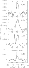 |
Fig. 4 Averaged NH3 spectra from April and May 2023. Channel widths are 0.48, 0.61, 0.50. and 0.64 km s–1 from top to bottom. |
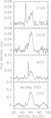 |
Fig. 5 Averaged NH3 spectra from April and May 2023. Channel widths are 0.54, 0.47, 0.55, and 0.45 km s–1 from top to bottom, respectively. |
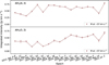 |
Fig. 6 Comparison of integrated intensities of the (5,3) and (6,3) maser features. “M” denotes “maser”, for which the velocity is given. Note that here and in the following plots the timescale (x axis) is not linear but is designed with equal spacings between consecutive observing epochs. Errors are standard deviations from Gaussian fits. |
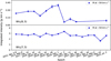 |
Fig. 7 Comparison of integrated intensities of the (7,5) and (8,5) maser features. For more details, see Fig. 6. |
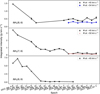 |
Fig. 8 Comparison of integrated intensities of the (6,6), (7,6) and (8,6) maser features. For more details, see Fig. 6. |
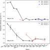 |
Fig. 9 Comparison of integrated intensities of the (10,9) and (11,9) maser features. For more details, see Fig. 6. |
3.4.3 Variability on shorter timescales
As already noted in Sect. 3.1, there are comparatively short periods with several obtained spectra between January 24, 2018, and February 1, 2018, as well as in April and May 2023. For the bulk of the measured maser features, i.e., in particular for those which are strong enough to be detected at individual epochs with high signal-to-noise ratios, we do not see any significant changes within the relatively short time intervals that cannot be explained by pointing and/or calibration errors. Significant differences in lineshapes are not obvious. This also holds for the (5,4) line during Dec 27–29, 2019 (Fig. A.5), as well as for the (9,6) line data with coarse spectral resolution (Figs. A.29 and A.30), even though this line is known to show the fastest variability (e.g., Henkel et al. 2013). For the (9,6) and (10,7) lines we have an additional large number of monitoring epochs with high velocity resolution, encompassing 2022 and 2023 (Figs. A.31, A.32, A.39, and A.40). Here we find slight differences in the (9,6) inversion line between March 17 and May 9, 2013, near VLSR = 56 km s–1, as well as between May 4 and June 17, 2022, near 59 km s–1. Indications for polarized line components as reported by Henkel et al. (2013) are not found. There are also small but notable differences between November 25, 2022, and February 7, 2023. The high spectral resolution data from the (10,7) line do not show such changes.
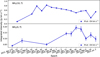 |
Fig. 10 Comparison of integrated intensities of the (9,7) and (10,7) maser features. For the (9,7) line, the average for the epochs between January 24 and February 1, 2018, was set to January 26. For more details, see Fig. 6. |
3.4.4 Additional ammonia features
There are a few spectral features that do not fully match the general trends outlined above. In the (5,4), (7,6), (7,7), (8,6), and (11,9) transitions, two neighboring features are occasionally detected. Earliest evidence for it is seen in the (7,7) lines in 2012 and 2013, where the 45 km s–1 component is accompanied by a ≈50 km s–1 feature (Fig. A.23). The latter component is getting weaker and is absent in the most recent (7,7) spectra (Figs. 5 and A.24). The low-spectral-resolution profiles of the (5,4) line are not showing convincingly two maser features (Figs. A.4 and A.5). However, the high-resolution spectra taken in 2019 and 2020 are clearly separating the components (Fig. A.6). The (7,6) line also reveals both components, but only in 2023 (Fig. A.22). Particularly clear is the situation in the case of the (8,6) line, where a double feature is also seen in 2023, at ≈50 and 54 km s–1. Earlier, in 2018, a double feature at 48 and 54 km s–1 is observed. Finally, at the end of January 2018, a tentative double feature is observed in the (11,9) line. The velocities agree with those of the double feature of the (8,6) line observed during the same time.
3.5 SiO and NH3-VIB
The lines of vibrationally excited ammonia and the ground rotational SiO transitions in their first and second vibrationally excited states (Fig. 11) can be compared with the K-band ammonia features also measured in April 2013. In the SiO υ = 2 line, there is a narrow <1 km s–1 wide feature at 54.1 km s–1, which is offset by a few 100 m s–1 from our so-called 54 km s–1 maser component from ammonia, i.e., those seen in the (7,4) and (8,5) transitions (Table B.1). We should note that the levels giving rise to the υ=2 emission are located at ≈3520 K above the ground state and thus far above those of the K-band ammonia lines discussed throughout this paper. Therefore the SiO υ=1 line with ≈1770 K is closer in excitation. And here we find at 54.6 km s–1 a broader component (≈2 km s–1), which matches the corresponding ammonia feature in a better way. Note, however, that according to Goddi et al. (2015), the NH3 and SiO masers are offset by 0.″65.
The (0,0) → (1,0) transition from the υ2 = 1 state of ammonia, the lowest vibrationally excited level of NH3, is located about 1400 K above ground and thus comparable in excitation to SiO υ = 1 or the previously measured (J, K) = (12,12) line of ammonia in the ground vibrational state (e.g., Henkel et al. 2013). The above mentioned υ2 = 1 ammonia line near 466 GHz is the equivalent to the ground state υ2 = 0, (1,0) → (0,0) line and shows, as the K = 0 ladder in the vibrational ground state, no inversion doubling. The profile shown in Fig. 11 (lowest panel) is not dominated by distinct narrow spectral features but by a single wide component covering approximately 20 km s–1 and peaking right at the systemic velocity of the source. Thus we are not able to connect the line profile to specific K-band λ ≈ 1.3 cm ground state maser lines. Instead, it covers the velocity range encompassed by the ground state (9,6) line.
We applied Eq. (1) of Schilke et al. (1992), i.e.,
 (1)
(1)
with kB denoting the Boltzmann constant, vul being the frequency and μ representing the dipole moment, 1.25 Debye. Taking the integrated intensity from Table B.20, we thus obtain for the upper state of the observed transition, the (0,0) level, Nu ≈ 1.3×1012 cm–2. With the partition function for Tex = 300 K,
 (2)
(2)
(see footnote4), and a statistical weight of 2 because the line is an ortho-NH3 transition, this leads to a total population of about N(υ2 = 1) ≈ 3.8 × 1014 cm–2 inside the 13″ sized beam of the APEX telescope. Realistically, however, the emission must arise from a much smaller region. Mauersberger et al. (1987) report a source size of 1.″26 for the quasi-thermal (7,7) line. Goddi et al. (2015) provide consistent results for some other highly excited metastable (J = K) lines. Adopting an angular size of order 1″ for the υ2 = 1, (0,0) → (1,0) transition, we thus obtain a column density of N(υ2=1,1″) ≈ 6.4 × 1016 cm–2. For the ground vibrational level, Mauersberger et al. (1987) find N(υ2=0) ≈2 × 1019 cm–2 for a 1″ beam. Aiming at the vibrational temperature, we then find with
 (3)
(3)
Tvib ≈ 250 K. This is very similar to the rotational temperature obtained by Mauersberger et al. (1987) and can be taken as an indication, that the υ2=1 line is not highly opaque. As a cautionary remark, however, we should also note that the submillimeter continuum at the frequency of the line, ≈466 GHz, may be optically thick, thus contaminating comparisons between the υ2 = 1 and the ground vibrational state which is studied at likely more transparent radio frequencies.
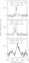 |
Fig. 11 Top panel: SiO J = 1→0 υ = 2 on a Jy scale. Middle panel: SiO J = 1→0 υ = 1 on a Jy scale. Bottom panel: NH3-VIB on a Tmb scale. Adopted frequencies are 42.82049, 43.12203, and 466.2452 GHz from the CDMS catalog (Müller et al. 2001, 2005; Endres et al. 2016). Channel spacings are 0.68, 0.68 and 0.39 km s–1 from top to bottom. In the case of the Gaussian fits outlined in Table B.20 of Appendix B, unsmoothed spectral profiles with velocity spacings of 0.17 km s–1 have been used for the SiO data. |
4 Discussion
4.1 Maser line saturation
For many NH3 inversion transitions the line widths of the maser profiles remained an unknown quantity. This was mainly related to the spectral resolution of the data presented by Henkel et al. (2013). Their channel widths were of order of 1 km s–1 or higher. The data presented here offer higher-spectral-resolution profiles, providing accurate line widths for several of the measured maser features (see Tables B.1–B.6).
Line widths well below 1 km s–1 could be convincingly determined in the case of the (5,3), (5,4), (6,3), (7,4), (8,5), (9,7), and (10,7) transitions. In the case of the 45 km s–1 features we find full width at half maximum (FWHM) line widths which are all around 1 km s–1. For the 54 km s maser components line widths are in the range of 0.3–0.6 km s–1 in the (7,4) (8,5), (9,7), and (10,7) transitions, but only ≈0.1 km s–1 in the (5,4) transition (see Fig. A.6). This is possible, because the main hyperfine components of the (5,4) transition only cover about 0.015 km s–1, a situation similar to that of the (10,7) line as discussed later in this section. Finally, for the 57 km s–1 features, line widths range between 0.4 and 0.8 km s–1 in the (5,3), (5,4), and (6,3) transitions. The similarity of line widths of each of the individual kinematical features (with the notable exception of the ultranarrow 54 km s–1 (5,4) feature) may support our assumption that many of the lines arise inside the same volume of gas.
With the equation of radiative transfer in the Rayleigh-Jeans limit, we obtain
 (4)
(4)
adopting an excitation temperature of Tex < 0 as is required for maser emission. Further assuming a Gaussian distribution of the optical depth as a function of velocity,
![Mathematical equation: $\tau = {\tau _0} \times {{\rm{e}}^{ - 4\ln 2{{\left[ {\left( {V - {V_0}} \right)/\Delta V} \right]}^2}}},$](/articles/aa/full_html/2025/08/aa54839-25/aa54839-25-eq12.png) (5)
(5)
we then get for the FWHM line width,
![Mathematical equation: $\Delta {V_{{\rm{maser}}}} = 2\Delta V{\left[ {{{ - \ln \left( { - \tau _0^{ - 1} \times \ln \left( {1 + {T_{{\rm{line}}}}/2} \right)} \right)} \over {4\ln 2}}} \right]^{1/2}}.$](/articles/aa/full_html/2025/08/aa54839-25/aa54839-25-eq13.png) (6)
(6)
Here, Tline is the peak line temperature at optical depth τ0 and ΔV is the FWHM line width in the case of non-inverted level populations. As a result, the maser line becomes, with rising absolute opacity, narrower than it would be under quasi-thermal conditions with positive excitation temperature and opacity. This is visualized in Fig. 12.
By far the best data allowing for a comparative analysis of line width versus line intensity are provided by our high spectral resolution monitoring of the (10,7) inversion line in 2022 and 2023 (see Figs. A.39 and A.40 and Table B.6). Fig. 13 shows the corresponding plot. What we find is a range in flux density by a factor of two accompanied by a change in line width of ≈ 14%. As expected, higher flux densities are leading to lower line widths. Connecting these observational data with the calculated changes shown in Fig. 12, we find a doubling of the flux density (assuming that the excitation temperature of the line does not vary) and a decrease in line width by 14% with opacities between –0.7 and –1.6. Note that this is more a qualitative than a quantitative estimate, mainly because of the only moderate change in line width. Not only that the excitation temperature might be changing, but there may also be small calibration errors even though the measurements were obtained with the same front- and backends. Furthermore, line intensities also depend on the pointing accuracy of the telescope. However, pointing errors <10″ (Sect. 2.1) do not allow for flux density variations by a factor of two. Pointing errors of 3, 5, and 7″, adopting a point-like maser source, only lead to flux density reductions of 1%, 3%, and 5% inside of a 50″ beam. Therefore a scenario of unsturated maser emission with an opacity of order –1 appears to be a suitable interpretation of the data obtained.
We have to note, however, that the considerations outlined above are only valid, if the strongest hyperfine components of the (10,7) transition are not encompassing a velocity range that is significant with respect to the observed line width. For unsat-urated masers it is helpful that the stronger hfs features are amplified more efficiently than the weaker ones, enhancing the discrepancy between weaker and stronger features (see, e.g., Agafonova et al. 2024). However, in the case of the (10,7) line the situation is clear. Using the JPL catalog5, we find six centrally located components, each of them stronger by at least two orders of magnitude than the ten individual hfs components ≳3 km s–1 on each side. These six strong hfs features only cover a velocity range ≈0.01 km s–1, i.e., their velocity coverage is indeed negligible with respect to the measured linewidth.
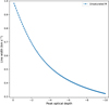 |
Fig. 12 Narrowing of an unsaturated maser feature with a full width at half maximum (FWHM) of 1 km s–1 as a function of peak optical depth, based on the Rayleigh–Jeans approximation of the equation of radiative transfer, Tline ∝(e–τ – 1), and a Gaussian distribution of opacity τ as a function of velocity. |
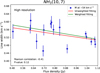 |
Fig. 13 NH3 (10,7) line widths as a function of line intensities. For the data, see Table B.6. The green and red lines represent linear fits to the weighted and unweighted data, respectively. |
4.2 Acceleration of the VLSR ≈ 45 km s–1 component
Henkel et al. (2013) reported that the lowest velocity maser component, their “45 km s–1” feature, showed a secular drift of ≈0.2 km s–1 yr–1 toward higher velocities, presumably due to an accelerated outflow also seen in SiO (Eisner et al. 2002). The monitoring was performed between 1996 and 2012. Our more recent data encompassing the following decade reveal a more complex picture.
From Fig. 14 we can see that there is an overall trend toward 48 km s–1, as seen in the (7,7), (7,6) and (11,9) transitions. However, this infers a much lower drift velocity than observed before, a drift at the order of 0.07 km s–1. In addition, there are other lines which show quite a different behavior. The (6,6) line drifted upward between 2013 and 2017 by about 2 km s–1 or created a new feature while the one at lower velocity faded. The difference in velocities is even more pronounced in the (8,6) line, where the velocity is rising from ≈46 km s–1 to 51–52 km s–1 between 2013 and 2023. In view of the lines, where the shift in velocity seems to be drastically enhanced during the last decade, we find it likely that the former maser feature has disappeared to be replaced by another one at higher velocity.
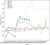 |
Fig. 14 Radial velocity of the so-called VLSR = 45 km s–1 component as a function of time for various NH3 inversion lines. |
4.3 The (J,K) = (9,6) as a special case
As mentioned, the (9,6) line is the fastest varying and strongest ammonia inversion line (see Figs. A.29–A.32). The main spike is found, in agreement with Zhang et al. (2022), at velocities near 54 km s–1, slightly above this value in 2013 to decrease slightly below this value in 2022 and 2023 (see also Sect 3.4.1). This is not seen in the 54 km s–1 features of other lines observed with high spectral resolution. The components near 60 km s–1 did also shift to slightly lower velocities. Noteworthy is in particular the emission below 50 km s–1, which can be found in the high spectral resolution plots of Figs. A.31 and A.32, which has to our knowledge not been reported before. The most recent spectra show components near 49 and even 47 km s–1. The latter emission corresponds to that seen also in other lines as shown in Fig. 14, leading to a velocity component observed in four consecutive inversion lines along the same K-ladder, i.e., the (6,6), (7,6), (8,6), and (9,6) transitions. We have to note, however, that the corresponding components of the (6,6) and (8,6) lines have disappeared at these epochs.
4.4 Para- and ortho-NH3 masers
The recent survey by Yan et al. (2024) revealed that in most massive star formation regions with NH3 masers, either solely para- or ortho-NH3 maser transitions could be identified. Only one of their 14 newly discovered NH3 maser sources revealed inverted populations in both NH3 maser species. Clearly, W51-IRS2 reveals maser lines from both ammonia species. However, this may only be due to the superposition of different maser hotspots in our single-dish beam (see, e.g., our Fig. 2 and Fig. 5 in Zhang et al. 2024b). For the so-called 45 km s–1 components we find inverted population in the (6,6), (7,6), (7,7), (8,6), (10,9) and (11,9) spectra (see Sect. 3.4). Furthermore, Henkel et al. (2013) reported corresponding features also in the (9,9) and (12,12) transitions. So this component reveals almost exclusively ortho-NH3 masers with the notable exception of the (7,7) line. The 54 km s–1 feature is seen in the (6,2), (7,3), (7,4), (7,5), (8,5), (9,7), (9,8), and (10,7) lines (Sect. 3.4). So this is an opposite case to that of the 45 km s–1 component. All lines belong to the para-NH3 species except the (7,3) transition. 57 km s–1 features are seen in the (5,2), (5,3), (5,4), (6,3), and (6,4) line. Here both para- and ortho-NH3 are contributing.
The preferences for either para- or ortho-NH3 might be explained by column density effects, because ortho-NH3 levels are characterized by twice the statistical weights of their para-counterparts, thus requiring lower column densities to reach optical depths yielding noticeable exponential maser amplification in cases of unsaturated maser emission (see Sect. 3.4.2). However, such an explanation may allow for deviations from the rule, since a factor of two in the statistical weights is not very much.
4.5 Comparison with other data
Following, for example, Goddi et al. (2015) and Zhang et al. (2024b), the warm molecular gas in W51-IRS2 shows a structure that is elongated along an east-west axis, including W51-N4, W51-d2, W51-N2, and W51-North from west to east, encompassing about 6″ (0.15 pc) at the southern edge of the more extended HII region W51d (Fig. 2). This includes the so-called Lacy-jet (Lacy et al. 2007), representing ionized gas, which originates in W51-N4, i.e., in the west, and extends eastward across the other above mentioned sub-sources (see, e.g., the upper left panel of Fig. 8 in Zhang et al. 2024b).
With respect to the discussion in Sect. 4.4, we thus may ask whether the 57 km s–1 maser features, representing both para-and ortho-NH3 transitions, arise from different regions inside W51-IRS2. Unfortunately, high angular resolution NH3 data provide so far only one maser line with emission near 57 km s–1. It is the (J, K) = (6,3) ortho-NH3 transition, reported by Zhang et al. (2024b), and observed toward W51d2 (their Fig. 3). While we have no accurate position for a corresponding para-NH3 line, it may be possible that such maser lines might arise from W51-North, located about 3.″5 eastward, because this is the region where most of the W51-IRS2-masers originate (e.g., Goddi et al. 2015; Zhang et al. 2024a). For example, the “45 km s–1” masers are observed at this position.
A monitoring program during January to April, 2020, involving four epochs and tracing the molecular species ammonia, water, and methanol was presented by Zhang et al. (2022). They used the Shanghai 65 m Tianma Radio Telescope (TMRT) with beam sizes of order 50″ to 60″ (see Fig. 1) and 3σ noise levels of ≈0.5 Jy in a single channel covering 0.043 km s–1. The epochs include early January, mid of March and early April and report a burst of line emission in some specific maser transitions. Fortuitously, the first epoch, January 8, 2020, used by Zhang et al. (2022) near the peak of the H2O maser flare is quite close to January 3, 2020, when we also covered the entire 18–26 GHz K-band spectrum (for a visualization, see Fig. 15). Zhang et al. (2022) reported rapidly increasing and decreasing line fluxes for several of our maser lines, but also for the quasi-thermal ones. In addition, they reported absorption features at ≈60 km s–1 on April 7.
Comparing our data from January 3, 2020, with those by Zhang et al. (2022) taken five days later, we can check some of their results in the light of our spectra. Zhang et al. (2022) reported a tentative (J, K) = (8,7) maser feature that is not confirmed by our data. While we see, like Zhang et al. (2022), more than one velocity feature in the (5,4), (7,6) and (9,6) maser lines, we do not find (unlike Zhang et al. 2022) more than a single nonthermal velocity component in the (7,5) transition. Confirming Zhang et al. (2022), there are also single maser components in the (5,3), (7,3), (8,6), and (10,7) lines on January 3, 2020, with our (8,6) line data revealing two velocity components at earlier and later epochs. The (9,7) and (9,8) lines are not detected by us during the critical time interval discussed here. Our decade-long monitoring observations never revealed any absorption line. Thus we do not find any supporting evidence for the (4,1), (4,2), (5,2), (5,3), (6,4), (8,6), and (9,6) absorption features reported by Zhang et al. (2022) near VLSR = 60 km s–1 as we can also not confirm variability in the quasi-thermal lines (see Sect. 3.1).
While there is good agreement with the absence of (6,6) maser emission and only weak maser emission in the (10,9) line in January 2020, another potential discrepancy is related to the (7,7) transition. The non-detection of the (7,7) maser by Zhang et al. (2022) is not compatible with our Sν ≈0.3 Jy detection only five days prior to their first epoch unless the maser is varying on very rapid timescales, which is not apparent in our longer term monitoring data.
Following the peak flux densities given in Zhang et al.’s (2022) Fig. 5 and our data from an epoch only five days earlier (January 3, 2020), we find good agreement in the (5,3), (6,2) and (7,3) transitions, moderate agreement in the (8,6) line, and clear disagreement in the (5,4), (6,3), (7,5) and (7,6) maser features. We suspect that these differences are not predominantly caused by maser variability in view of our short timescale analysis provided in Sect. 3.4.3. Thus we are viewing the data of Zhang et al. (2022) with some skepticism and suggest that variability is not as extreme and fast as suggested in their analysis from spectra taken in early 2020.
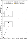 |
Fig. 15 All of the NH3 maser features detected by Zhang et al. (2022) and this study in January 2020. Note that our data were taken on January 3, while those of Zhang et al. (2022) were obtained on January 8. |
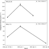 |
Fig. 16 Variability of the integrated intensities of the (7,7) and (11,9) lines between 2018 and 2023. |
4.6 Heat waves and flaring events
As already mentioned in Sect. 4.5, Zhang et al. (2022, 2024a) reported luminosity outbursts in H2O, NH3 and CH3OH maser lines in early 2020. With our data from 2020, January 3, we can check whether our maser lines are flaring with respect to early 2018, i.e., two years earlier, and April 2023, about three years afterward. Our results turn out to be mostly “disappointing”. Among the maser features with sufficient signal-to-noise ratios to be analyzed in this context, the (5,3), (5,4), (6,3), (7,3), (7,4), (7,5), (7,6), (8,6), (9,6), and (10,7) transitions show no significant increases in flux density in early 2020. Only the (7,7) and (11,9) lines show such an effect (Fig. 16). Integrated (7,7) maser line intensities in units of Jy km s–1 are 0.342±0.022 on February 1, 2018, 0.811 ±0.041 on January 3, 2020, and 0.067±0.020 on April 26, 2023 (Table B.14). For the (11,9) line we find correspondingly 0.073±0.010 (Jan. 24 to Feb. 1, 2018), 0.268±0.025 (Jan. 3, 2020) and 0.099±0.12 (Apr. 11, 2023) in Table B.19. To conclude, we do not see a general flare in the ammonia maser lines in early 2020.
A longer monitoring time span from 2020 till 2023, available for the 22 GHz H2O line, was reported by Volvach et al. (2023). Their data, obtained with an angular resolution of 150″ and thus potentially including W51-IRS1 (see Fig. 1), reveal a strong flare between late 2021 and early 2022, peaking approximately in January 2022 (their Fig. 1). Zhang et al. (2024a) reported that the bulk of this flare likely originates from a compact disk-like structure in W51-North, the eastern part of W51-IRS2. The 22 GHz H2O transition connects levels ≈640 K above the ground state which is compatible with several of our ammonia masers (see Table 1). We may therefore ask whether we can find any evidence for this flare also in our NH3 data.
We present observations in early 2022 for the (9,6) and (10,7) lines. These are two particularly highly excited NH3 inversion lines connecting levels >1000 K above the ground state (Table 1). While the peak flux density of the water maser flare was about 140 kJy, which is four orders of magnitude more powerful than the most intense maser component we detected in this study, H2O flux densities decrease from ≈20 kJy in early March 2022 to ≈ 15 kJy till the end of June to then briefly rise to 30 kJy in early July, decreasing then once more to 15 kJy, rising then during the last months of the year to 20–25 kJy to then fade to normal levels of a few kJy. In our high spectral resolution data of the (9,6) transition (Figs. A.31 and A.32) we do not see any correlated variability. This also holds for the (10,7) masers presented in Figs. A.39 and A.40. It should be noted here, that the NH3 masers in W51-IRS2 may be pumped by infrared radiation (see Sect. 3.4.2), while the H2O masers are believed to be collisionally excited (e.g., Kylafis & Norman 1987, 1991). This might lead to delayed H2O maser flare episodes with respect to NH3, also depending on the detailed spatial configuration.
Zhang et al. (2022) interpreted variability in terms of rather shortlived accretion episodes, leading to heatwaves and to maser flares in the surrounding energized medium. What we have found is a maser flare identified on much larger timescales. With respect to the so-called 45 km s–1 component, emission was strongest during the initial epochs (see Henkel et al.’s 2013 Figs. 1–3 and our Appendix A). Originally discovered in the ammonia (9,9) and (12,12) lines of orthe-NH3 in November and December 1995, the multilevel ammonia study of Mauersberger et al. (1987) presenting spectra from 1985 and 1986 does not show any emission at this velocity. The (9,9) and (12,12) lines showed increased line intensities in late August of 2011 (Henkel et al. 2013). The lines studied here with sufficient signal-to-noise ratios are the (6,6), (7,6), (7,7), (8,6), (11,9) transitions. What is common to their maser features is a slowly advancing decay, which appears not to be monotonic but proceeds in distinct steps. The earliest measurements of the (6,6), (7,6), (7,7) masers were taken in 2008. For the (8,6) and (11,9) lines, the starting point is early April 2012. Strongest line emission was seen in October 25, 2008 (Henkel et al. 2013), and in 2012 in the case of the (6,6) and (7,6) lines, which is compatible with the (9,9) and (12,12) maser lines, which were stonger in 2011 than during their discovery in 1995. While the (7,7) transition fades already by a factor of about eight between 2008 and 2012, the (6,6), (7,6) and (8,6) lines only get clearly weaker during 2013. By 2020, the (6,6) line is gone. The (7,7) line is not clearly detectable after 2020, while the (8,6) line stays at a constant level of ≈0.25 Jy. The latter also holds for the (11,9) transition, only that here the resulting flux densities are below 0.1 Jy. And the (9,6) transition starts to show weak emission at velocities slightly below 50 km s–1.
To summarize, the feature may have risen for at least 15 years from 1995 till about 2010, while it was not yet apparent in 1985 and early 1986 (Mauersberger et al. 1987). Beginning in 2013, the lines became weaker. Here it is interesting that the line with lowest excitation, the (6,6) transition, is fading first, while the (8,6) and (11,9) transitions still show the feature in 2023. During this year, also weak (9,6) emission at VLSR < 50 km s–1 is appearing. Instead of a heat wave which expands and successively excites lines of lower energy above the ground state, here we seem to have the opposite with only the lines with highest excitation still being found to be masering. Not knowing exact physical boundary conditions nor having detailed radiative transfer calculations involving vibrational excitation, we propose the following tentative explanations:
We may assume the presence of two sources, one emitting the maser lines at lower levels above the ground state, and the other longer lived source providing emission from the higher J levels. Since both emit at velocities, which cannot be distinguished, and since both were appearing during the same, admittedly large time interval, this appears to be not likely. Furthermore, Goddi et al. (2015) demonstrated that the low velocity (blue) (6,6), (7,7), and (9,9) line components originate from the same location. Potential differences in position are not larger than a few milli-arcsec (≈20 AU);
The possibility that infrared line overlaps play a significant role is also not likely. This is due to the fact that only the (9,6) line intensities appear to be exceptional, thus offering the possibility that this but only this line is affected by such overlaps (e.g., Madden et al. 1986). Also, here we have several lines with lower and higher J quantum numbers. Similar line overlap effects for several of these transitions are unlikely;
Considering the timescales involved, rotation of a molecular cloud is yet another option (e.g., Gray et al. 2019). When the (6,6) and (7,7) lines would arise farther away from the exciting source, then they might leave first the line-of-sight to a compact background source they may amplify. Or the maser cones of the (6,6), (7,6) and (7,7) lines are narrower than those of the (8,6) and (11,9) transitions;
Intuitively, one may think that masers from lines closer to the ground state are always emitting from hotspots farther away from the central irradiating source than the higher J ones. However, there exists a counter-example: The SiO υ =1 J = 2→1 masers are occasionally observed at larger distances from the central source than the corresponding J = 1→0 lines, representing a lower degree of rotational excitation. This holds in the case of the SiO maser sources in Orion-KL and the late type stellar object IRC+10011 (e.g., Soria-Ruiz et al. 2004; Issaoun et al. 2017). If this is also valid for our ammonia masers, then a passing heat wave might quench the inner maser lines from lower J states earlier than those from higher J levels farther out.
In the case of the other maser features we lack information on the epoch when they formed. This also holds for our tentatively detected (5,2) and (6,4) masers at ≈57 km s–1, which – if real – may have been too weak to be detectable in previous studies. Furthermore, the flux densities of the masers at >50 km s–1 do not follow a sufficiently regular pattern that is comparable to that of the so-called 45 km s–1 feature. Therefore we cannot provide related scenarios potentially explaining their variability.
5 Conclusions
We have presented data from the numerous detected ammonia masers in W51-IRS2. Some of the key findings of this study are:
(1) We present the first tentative discovery of a (J,K) = (5,2) ammonia maser in the interstellar medium. Tentatively, a (6,4) maser is seen for the first time in W51-IRS2, while, also for the first time, (9,6) maser emission is detected at local standard of rest velocities <50 km s–1 in this source;
(2) The data taken during the time interval from 2012 to 2023 demonstrate that previously determined peak flux densities are roughly confirmed, because most of the maser lines have full width at half maximum line widths of ≈ 1 km s–1;
(3) The distribution of maser lines in the NH3 level diagram shows strong hints for being pumped by infrared radiation;
(4) Vibrationally excited ammonia is indeed detected, suggesting a vibrational excitation temperature, which is compatible with the kinetic temperature of ≈300 K;
(5) Analyzing the (10,7) maser features over a time interval of ≈15 months, a weak correlation between line width and intensity is found, which is consistent with unsaturated maser emission and a peak optical depth of order –1;
(6) The previously reported velocity drift of the so-called 45 km s–1 maser component has slowed down considerably or is even absent in most recent spectra. Furthermore, the maser lines from this component connecting levels <800 K above the ground state disappear during the observed time interval, while the lines with highest excitation, the (8,6), (9,6) and (11,9) lines still show features at <50 km s–1 till 2023. Tentative interpretations are provided;
(7) For early 2018 and during April and May 2023, when monitoring took place on almost daily or weekly basis, no sudden and/or strong variability is seen. No absorption line is found. A correlation of ammonia maser lines with a strong 22 GHz H2O flare is not found. The 54 km s–1 features show highly inconsistent variability patterns. It is suggested that they may arise from more than one active region in W51-IRS2.
Data availability
Appendices A (containing 44 figures with the monitored spectra) and B (including 20 tables presenting Gaussian fits to the spectra) are available at https://zenodo.org/records/15746097.
Acknowledgements
We wish to thank the people at Effelsberg for their great support, in particular B. Winkel and A. Kraus, when analyzing the 8 GHz wide spectra from early 2018. We also profited from discussions with T. Krichbaum and B. Lankhaar. Finally, we wish to thank the referee for good and helpful comments further improving the paper. E. Alkhuja was supported by King Abdulaziz University and the Cultural Office of the Embassy of the Kingdom of Saudi Arabia in Berlin. Related to A. Wootten: The National Radio Astronomy Observatory and Green Bank Observatory are facilities of the U.S. National Science Foundation operated under cooperative agreement by Associated Universities, Inc. This research has made use of NASA’s Astrophysical Data System.
References
- Agafonova, I. I., Bayandina, O. S., Gong, Y., et al. 2024, MNRAS, 533, 1714 [Google Scholar]
- Beuther, H., Walsh, A. J., Thorwirth, S., et al. 2007, A&A, 466, 989 [NASA ADS] [CrossRef] [EDP Sciences] [Google Scholar]
- Bisschop, S. E., Jørgensen, J. K., van Dishoeck, E. F., & de Wachter, E. B. M. 2007, A&A, 465, 913 [NASA ADS] [CrossRef] [EDP Sciences] [Google Scholar]
- Brown, P. D., Charnley, S. B., & Millar, T. J. 1988, MNRAS, 231, 409 [Google Scholar]
- Caselli, P., Hasegawa, T. I., & Herbst, E. 1993, ApJ, 408, 548 [Google Scholar]
- Cesaroni, R., Walmsley, C. M., & Churchwell, E. 1992, A&A 256, 618 [NASA ADS] [Google Scholar]
- Charnley, S. B., Tielens, A. G. G. M., & Millar, T. J. 1992, ApJ, 399, L71 [Google Scholar]
- Demes, S., Lique, F., Loreau, J., & Faure, A. 2023, MNRAS, 524, 2368 [NASA ADS] [CrossRef] [Google Scholar]
- Eisner, J. A., Greenhill, L. J., Herrnstein, J. R., Moran, J. M., & Menten, K. M. 2002, ApJ, 569, 334 [CrossRef] [Google Scholar]
- Endres, C. P., Schlemmer, S., Schilke, P., Stutzki, J., & Müller, H. S. P. 2016, J. Mol. Spectr. 327, 95 [NASA ADS] [CrossRef] [Google Scholar]
- Garrod, R. T., & Widicus Weaver, S. L. 2013, ChRv, 113, 8939 [Google Scholar]
- Gaume, R. A., Wilson, T. L., & Johnston, K. J. 1996, ApJ, 457, L47 [NASA ADS] [Google Scholar]
- Genzel, R., Ho, P. T. P., Bieging, J., & Downes, D. 1982, ApJ, 259, L103 [Google Scholar]
- Ginsburg, A., Goss, W. M., Goddi, C., et al. 2016, A&A, 595, A27 [NASA ADS] [CrossRef] [EDP Sciences] [Google Scholar]
- Goddi, C., Henkel, C., Zhang, Q., Zapata, L., & Wilson, T. L. 2015, A&A, 573, A109 [NASA ADS] [CrossRef] [EDP Sciences] [Google Scholar]
- Gray, M. D., Baggott, J., Westlake, J., & Etoka, S. 2019, MNRAS 486, 4216 [NASA ADS] [CrossRef] [Google Scholar]
- Guilloteau, S., Wilson, T. L., Martin, R. N., Batrla, W., & Pauls, T. A. 1983, A&A, 124, 322 [NASA ADS] [Google Scholar]
- Güsten, R., Nyman, Å., Schilke, P., et al. 2006, A&A, 454, L13 [NASA ADS] [CrossRef] [EDP Sciences] [Google Scholar]
- Henkel, C., Jacq, T., Mauersberger, R., Menten, K. M., & Steppe, H. 1987, A&A, 188, L1 [NASA ADS] [Google Scholar]
- Henkel, C., Wilson, T. L., Asiri, H., & Mauersberger, R. 2013, A&A, 549, A90 [NASA ADS] [CrossRef] [EDP Sciences] [Google Scholar]
- Howard, E. M., Koerner, D. W., & Pipher, J. L. 1997, ApJ, 477, 738 [Google Scholar]
- Issaoun, S., Goddi, C., Matthews, L. D., et al. 2017, A&A, 606, A126 [NASA ADS] [CrossRef] [EDP Sciences] [Google Scholar]
- Klein, B., Hochgürtel, S., Krämer, L., et al. 2012, A&A, 542, L3 [NASA ADS] [CrossRef] [EDP Sciences] [Google Scholar]
- Klein, T., Ciechanowicz, M., Leinz, C., et al. 2014, IEEE, 4, 588 [Google Scholar]
- Kylafis, N. D., & Norman, C. 1987, ApJ, 323, 346 [NASA ADS] [CrossRef] [Google Scholar]
- Kylafis, N. D., & Norman, C. 1991, ApJ, 373, 525 [Google Scholar]
- Lacy, J. H., Jaffe, D. T., Zhu, Q., et al. 2007, ApJ, 658, L45 [NASA ADS] [CrossRef] [Google Scholar]
- Loreau, J., Faure, A., Lique, F., Demes, S., & Dagdigian, P. J. 2023, MNRAS, 526, 3213 [Google Scholar]
- Madden, S. C., Irvine, W. M., Mathhews, H. E., Brown, R. D., & Godfrey, P. D. 1986, ApJ, 300, 79 [Google Scholar]
- Mangum, J. G., & Wootten, A. 1994, ApJ, 428, L33 [NASA ADS] [CrossRef] [Google Scholar]
- Mauersberger, R., Henkel, C., Wilson, T. L., & Walmsley, C. M. 1986a, A&A, 162, 199 [Google Scholar]
- Mauersberger, R., Wilson, T. L., & Henkel, C. 1986b, A&A, 160, L13 [NASA ADS] [Google Scholar]
- Mauersberger, R., Henkel, C., & Wilson, T. L. 1987, A&A, 173, 352 [NASA ADS] [Google Scholar]
- Mauersberger, R., Wilson, T. L., & Henkel, C. 1988, A&A, 201, 123 [NASA ADS] [Google Scholar]
- Mei, Y., Chen, X., Shen, Z.-Q., & Li, B. 2020, ApJ, 898, 157 [NASA ADS] [CrossRef] [Google Scholar]
- Mills, E. A. C., Ginsburg, A., Clements, A. R., et al. 2018, ApJ, 869, L14 [NASA ADS] [CrossRef] [Google Scholar]
- Müller, H. S. P., Thorwirth, S., Roth, D. A., & Winnewisser, G. 2001, A&A, 370, L49 [Google Scholar]
- Müller, H. S. P., Schlöder, F., Stutzki, J., & Winnewisser, G. 2005, J. Mol. Struct., 742, 215 [Google Scholar]
- Ott, M., Witzel, A., Quirrenbach, A., et al. 1994, A&A, 284, 331 [NASA ADS] [Google Scholar]
- Pickett, H. M., Poynter, R. L., Cohen, E. A., et al. 1998, JQSRT, 60, 8 [Google Scholar]
- Sato, M., Reid, M. J, Brunthaler, A., & Menten, K. M. 2010, ApJ, 720, break 1055 [NASA ADS] [CrossRef] [Google Scholar]
- Schilke, P., Walmsley, C. M., & Mauersberger, R. 1991, A&A, 247, 516 [NASA ADS] [Google Scholar]
- Schilke, P, Güsten, R., Schulz, A., Serabyn, E., & Walmsley, C. M. 1992, A&A, 261, L5 [Google Scholar]
- Soria-Ruiz, R., Alcolea, J., Colomer, F., et al. 2004, A&A, 426, 131 [NASA ADS] [CrossRef] [EDP Sciences] [Google Scholar]
- Volvach, A. E., Volvach, L. N., & Larionov, M. G. 2023, ApJ, 955, 10 [Google Scholar]
- Wakelam, V., Selsis, F., Herbst, E., & Caselli, P. 2005, A&A, 444, 883 [NASA ADS] [CrossRef] [EDP Sciences] [Google Scholar]
- Walmsley, C. M., & Ungerechts, H. 1983, A&A, 122, 164 [Google Scholar]
- Walmsley, C. M., Hermsen, W., Henkel, C., Mauersberger, R., & Wilson, T. L. 1987, A&A, 172, 311 [NASA ADS] [Google Scholar]
- Walsh, A. J., Longmore, S. N., Thorwirth, S., Urquhart, J. S., & Purcell, C. R. 2007, MNRAS, 382, L35 [NASA ADS] [Google Scholar]
- Wilson, T. L., Batrla, W., & Pauls, T. 1982, A&A, 110, L20 [NASA ADS] [Google Scholar]
- Wilson, T. L., Henkel, C., & Hüttemeister, S. 2006, A&A, 460, 533 [NASA ADS] [CrossRef] [EDP Sciences] [Google Scholar]
- Yan, Y. T., Henkel, C., Menten, K. M., et al. 2022a, A&A, 659, A5 [NASA ADS] [CrossRef] [EDP Sciences] [Google Scholar]
- Yan, Y. T., Henkel, C., Menten, K. M., et al. 2022b, A&A, 666, L15 [NASA ADS] [CrossRef] [EDP Sciences] [Google Scholar]
- Yan, Y. T., Henkel, C., Menten, K. M., et al. 2024, A&A, 686, A205 [NASA ADS] [CrossRef] [EDP Sciences] [Google Scholar]
- Zhang, Y.-K., Chen, X., Sobolev, A. M., et al. 2022, ApJS, 260, 34 [NASA ADS] [CrossRef] [Google Scholar]
- Zhang, Y.-K., Chen, X., Song, S.-M., & Wang, Y.-X. 2024a, AJ, 166, 21 [Google Scholar]
- Zhang, Y.-K., Chen, X., Wang, Y.-X., et al. 2024b, AJ, 168, 10 [Google Scholar]
This publication is based on observations with the 100-m telescope of the MPIfR (Max-Planck-Institut für Radioastronomie) at Effelsberg.
This publication is also based on data acquired with the Atacama Pathfinder Experiment (APEX), which was a collaboration between the Max-Planck-Institut für Radioastronomie (MPIfR), the European Southern Observatory (ESO), and the Onsala Space Observatory (OSO).
All Tables
All Figures
|
Fig. 1 Jansky Very Large Array continuum map of the W51 region at 14.5 GHz (image taken from Ginsburg et al. 2016; synthesized beam size: 0.″). W51d is associated with the northwestern hotspot, W51-IRS2, while the more extended bright region to the southeast is W51-IRS1. Our Effelsberg beam size of ≈40″ (the inner circle) encompasses the entire IRS2 region, but is small enough to exclude IRS1. The slightly larger circle, corresponding to 55″, refers to the beam size of the Tian Ma Radio telescope near Shanghai. |
| In the text | |
|
Fig. 2 Overlay of the 25 GHz continuum emission (gray scale and white contours) and the integrated intensities of the quasi-thermal (6,6) and (10,10) lines of ammonia (taken from Goddi et al. 2015). The (6,6) contours show the elongated dense molecular environment at the southern boundary of the H II region W51d. The location of main molecular hotspots, W51N4, W51d2, W51N2, and W51-North (from west to east), are indicated. For more details, see Goddi et al. (2015). |
| In the text | |
|
Fig. 3 Averaged NH3 spectra from April and May 2023. Channel widths are 0.60, 0.55, 0.61, and 0.56 km s–1 from top to bottom, respectively. |
| In the text | |
|
Fig. 4 Averaged NH3 spectra from April and May 2023. Channel widths are 0.48, 0.61, 0.50. and 0.64 km s–1 from top to bottom. |
| In the text | |
|
Fig. 5 Averaged NH3 spectra from April and May 2023. Channel widths are 0.54, 0.47, 0.55, and 0.45 km s–1 from top to bottom, respectively. |
| In the text | |
|
Fig. 6 Comparison of integrated intensities of the (5,3) and (6,3) maser features. “M” denotes “maser”, for which the velocity is given. Note that here and in the following plots the timescale (x axis) is not linear but is designed with equal spacings between consecutive observing epochs. Errors are standard deviations from Gaussian fits. |
| In the text | |
|
Fig. 7 Comparison of integrated intensities of the (7,5) and (8,5) maser features. For more details, see Fig. 6. |
| In the text | |
|
Fig. 8 Comparison of integrated intensities of the (6,6), (7,6) and (8,6) maser features. For more details, see Fig. 6. |
| In the text | |
|
Fig. 9 Comparison of integrated intensities of the (10,9) and (11,9) maser features. For more details, see Fig. 6. |
| In the text | |
|
Fig. 10 Comparison of integrated intensities of the (9,7) and (10,7) maser features. For the (9,7) line, the average for the epochs between January 24 and February 1, 2018, was set to January 26. For more details, see Fig. 6. |
| In the text | |
|
Fig. 11 Top panel: SiO J = 1→0 υ = 2 on a Jy scale. Middle panel: SiO J = 1→0 υ = 1 on a Jy scale. Bottom panel: NH3-VIB on a Tmb scale. Adopted frequencies are 42.82049, 43.12203, and 466.2452 GHz from the CDMS catalog (Müller et al. 2001, 2005; Endres et al. 2016). Channel spacings are 0.68, 0.68 and 0.39 km s–1 from top to bottom. In the case of the Gaussian fits outlined in Table B.20 of Appendix B, unsmoothed spectral profiles with velocity spacings of 0.17 km s–1 have been used for the SiO data. |
| In the text | |
|
Fig. 12 Narrowing of an unsaturated maser feature with a full width at half maximum (FWHM) of 1 km s–1 as a function of peak optical depth, based on the Rayleigh–Jeans approximation of the equation of radiative transfer, Tline ∝(e–τ – 1), and a Gaussian distribution of opacity τ as a function of velocity. |
| In the text | |
|
Fig. 13 NH3 (10,7) line widths as a function of line intensities. For the data, see Table B.6. The green and red lines represent linear fits to the weighted and unweighted data, respectively. |
| In the text | |
|
Fig. 14 Radial velocity of the so-called VLSR = 45 km s–1 component as a function of time for various NH3 inversion lines. |
| In the text | |
|
Fig. 15 All of the NH3 maser features detected by Zhang et al. (2022) and this study in January 2020. Note that our data were taken on January 3, while those of Zhang et al. (2022) were obtained on January 8. |
| In the text | |
|
Fig. 16 Variability of the integrated intensities of the (7,7) and (11,9) lines between 2018 and 2023. |
| In the text | |
Current usage metrics show cumulative count of Article Views (full-text article views including HTML views, PDF and ePub downloads, according to the available data) and Abstracts Views on Vision4Press platform.
Data correspond to usage on the plateform after 2015. The current usage metrics is available 48-96 hours after online publication and is updated daily on week days.
Initial download of the metrics may take a while.